An approximate approach of global optimization for polynomial programming problems

(1)

ELSEVIER

JOURNAL OF OPERATIONAL

RESEARCH European Journal of Operational Research 107 ( 1998) 625-632

Theory and Methodology

An approximate approach of global optimization

for polynomial programming problems

Han-Lin Li

* ,

Ching-Ter Chang

Institute of htformation Management, National Chiao Tung Uniuersiiy, Ta Hsieh Rd., Hsinchu 30050, Taiwan, ROC Received 28 March 1995; accepted 15 August 1996

Abstract

Many methods for solving polynomial programming problems can only find locally optimal solutions. This paper

proposes a method for finding the approximately globally optimal solutions of polynomial programs. Representing a bounded continuous variable xi as the addition of a discrete variable dj and a small variable E,, a polynomial term xixi can

be expanded as the sum of d,xj, dj&; and E,E,. A procedure is then developed to fully linearize din, and djci, and to

approximately linearize E;C~ with an error below a pre-specified tolerance. This linearization procedure can also be extended to higher order polynomial programs. Several polynomial programming examples in the literature are tested to demonstrate that the proposed method can systematically solve these examples to find the global optimum within a pre-specified error. 0 1998 Elsevier Science B.V.

Keywords: Global optimization; Linearization; Polynomial program

1. Introduction subject to

This paper develops a method for seeking a global g,(X)lO, k=l,..., q,

minimum of a polynomial program where the poly- _{X=(~*,...,X,),}

nomial terms may appear in the objective function

and the constraints. None of the convexity restric- OIf;IX,I~, i= l)..., n,

tions is imposed on these functions and constraints.

The mathematical expression of a polynomial pro-

where f,< X> and gk( X) are polynomial functions of

gramming problem is given below:

X, and f; and K are respectively the lower and the

upper bound of xi.

(PP Problem)

Some approaches for solving the above polyno-

mial programming problems are discussed below.

Global Min _C&(X)

i 1.1. Analytical approach

Horst and Tuy [5] proposed outer approximation

techniques for solving a PP Problem with Lips-

* Corresponding author. E-mail:hlli@ccsun2.cc.nctu.edu.tw. chitzian objective function and constraint. Hansen,

(2)

626 H.-L. Li, C.-T. Chang/European Journal of Operational Research 107 (1998) 625-632

Jaumard and Lu [3] developed interval analysis based

sufficient conditions for convergence, and provided

ways to eliminate variables and to reduce the ranges

of variables. These analytical approaches, however,

are only convergent in the absence of blocking sub-

problems. As the size of problems increases it be-

comes more and more likely that successive elimina-

tion of variables leads to problems too complicated

to allow any further elimination [3]. The analytical

approach is promising in finding a global optimum

of a PP Problem only if the range of variables of the

PP Problem can be easily reduced by analytical

techniques.

1.2. Concave minimization approach and binary ap-

proach

Particular cases of PP Problems, such as concave

programming problems and bilinear programming

problems, have attracted much attention. Work on

these problems was reviewed by Pardalos and Rosen

[ 111. Various O-l polynomial programs proposed by

Hansen, Jaumard and Lu [2] and Li [7,8] perform

well in finding globally optimal solutions. These

approaches exploit the special structure of the PP

Problem and therefore they are not directly applica-

ble to the general polynomial programming problems

discussed in this paper.

1.3. Stochastic approach

Many stochastic algorithms for global optimiza-

tion, such as the multistart with clustering [12,9]

used random search to converge asymptotically to a

global optimum. The algorithms can also be ex-

tended to find global solutions. This approach is

quite promising in searching for a global optimum in

highly nonlinear programs which are difficult to treat

by other methods. However, since this technique

requires evaluating a huge amount of starting points,

it can only be applied to solve small size problems.

1.4. Reformulation - linearization approach

Sherali and Tuncbilek [ 151 and Adams and Sherali

[ 141 derived a reformulation linearization technique

(RLT) which generated polynomial implied con-

straints, and subsequently linearized the resulting

problem by defining new variables. This construct

was then used to obtain lower bounds in the context of a proposed branch and bound scheme. Although

the RLT process is promising with respect to con-

verging to a global solution, the process is in practice

very difficult to implement owing to the following

reasons: (i) Several types of implied constraints, or

subsets, or surrogates need to be generated in a

linearized form. Tightening its representation at the

expense of an exponential constraint step by step is a

long trial and error process. (ii) The RLT algorithm always needs to generate a huge amount of bounded

constraints; many of these constraints are redundant.

(iii) These are considerable variants in designing a

RLT process, depending on the actual structure of

the problem being solved. A user needs to formulate

a special RLT scheme corresponding to each of his

programs.

This paper develops a new method for solving a

PP Problem and to find a global optimum with a

prespecified tolerance. The developed method uses a

convenient linearization technique to systematically

convert a PP Problem into a linear mixed O-l prob-

lem. The solution of this converted problem can be

as close as possible to the global optimum of the

original PP Problem. A comparison of this method

with other methods reviewed above is given below: 1. The proposed methods can solve general PP Prob-

lems. In contrast, the analytical approach [3] can

only solve problems in the absence of blocking

subproblems. The outer approximation techniques

[5] or concave minimization approach [l l] can

only treat problems with specific objective functions and constraints.

2. Both the proposed method and the multistart

method [ 12,9] can solve a PP Problem to obtain a

solution closing in on a global optimum. How-

ever, the multistart method requires evaluating a

huge amount of starting points.

3. The proposed method can systematically solve the

general PP Problem, but the reformulation-lineari-

zation approach [1_5] can only solve particular

problems using various RLT processes.

This paper has solved many test problems from

the compendiums of Hock and Schittkowski [4],

Schittkowski [6], and other sources. The experiment

demonstrates that the proposed method stably treats

all of the test problems in finding globally optimal

(3)

2. Preliminaries

Consider a bounded variable xi, 0 I li I xi 5 7,

where 1; and y are constants. xi can be represented

as follows:

.I

x; = Ii + w; c 2’-,yij + Ei, _(2.1)

j=l

where:

is the lower bound of xi.

is the pre-specified positive constant which is the

upper bound of ci, is a O-l variable.

is an integer which denotes the number of re-

quired O-l variables for representing xi.

is a small variable, 0 I E, < wi.

For any bounded variable xi, there is an unique

set of yi, (j = 1,. . . , J), oi and E, such that Eq.

(2.1) is satisfied. For example, if xi is a variable

between 10 and 15 and wi is chosen as 0.1, x, can

then be represented as

x,= lOfO.ly,, +o.2y,*+o.4yi,+o.8yi,

+ 1.6~~~ + 3.2~~~ + E,,

where O~.s,lO.l and yij, j= l,..., 6, are O-l

variables. Suppose xi = 13.752. Then Yi, = Y, 3 = Y, 6 = ’ 3

Yi2=Yj.$=Yi5=” and E; = 0.052.

Referring to Eq. (2.11, a polynomial term x, x2 is

represented as

x,x,=A,x,+~,x~

=A,x, +AZel + E,E~, _(2.2)

where

A, = 1; + wi i 2j-‘y,, for i= 1,2. _(2.3)

j=l

Define e12 as a linear approximation of E, E*, ex-

pressed as

e12 = 2 ‘(co,&* + lo*&,). (2.4)

The error of approximating E,B~ is computed as

0 I e12 - &,&2=~(0,&2+W2E,)-&,&2+iJ,W2

(2.5)

The maximal difference between e12 and E, c2 is

&,wz, which occurs at E, = $w, and ~2

= ?jw,.Substituting El E2 by e,2, expression (2.2)

can be approximately linearized as

x,x~=A,x?;+A~E,+&~J,E~+w,E,). _(2.6)

The following section will show that the polyno-

mial terms A, x2 and A, E, can be fully linearized.

The maximum error of approximately linearizing

x,x2 in Eq. (2.6) is therefore less than ~w,w,. By

specifying smaller w, and w2 values, a more accu-

rate approximation can be obtained. Choosing a

smaller o,, however, requires using more binary

variables to represent a bounded variable xi in Eq.

(2.1).

3. Linear strategies

A polynomial term x,x2 can be approximated as

follows, referring to Eqs. (2.2), (2.31, (2.4), (2.5) and (2.6):

J

XlX2=~,X2+W, C2’-‘y,,X,+&E,

i=l

J

f w2 C 2j-‘yZj6, + +( W,E~ + WOE,),

j=l

(3.1)

where I,, l,, w,, w2, I and J are constants, E, and

~2 are continuous variables, y,, and yZj are binary

variables, and 0 I Ed I wk, for k = 1,2. The terms

ylix2 and yzjg, in Eq. (3.1) can be fully linearized

based on Proposition 1 discussed below.

Proposition 1. Given a polynomial term

YlY,,..., y,,x, in which y, y,, . . . , y,, are binary

variables and 0 I x IX, with x a constant,

YlY29...’ y,, x can be fully linearized as Y,Y2?...>YnX=q,

where the following inequalities are satisfied

1. x+(y, +y2+ ... +y,-n)T<qIx;

2. OIq<Xy,, i= l,..., n.

This proposition can be checked as follows: If one

of the y,y,,..., y. equals 0, then q = 0; and if all

(4)

Proposition 2. Based on Proposition 1, a linear Replacing [x~x~I~&,~~-‘Y~~ by CkK_12k-1q3k,

approximation of x, x2, denoted as [x, x,], can be [x1x2x3] is then converted into the form expressed expressed as in Proposition 3.

[xx]=1,x2+w*

~2'-1q,;+1,El i= 1

+w*~2’-‘q*j+~(W1E*+WZEl),

j=l

where q, i and qzj are bounded by the following inequalities:

OIqliSX1yli, i= l,..., I,

X2(yli- l)XIqliIx,, i= l,..., I,

O(q,jIw*Y,,,

j=l,...,J,

El+(y2,-1)W1~q2j--<El, j=l,..., J.

It is clear that [x1 x2] 2 x1 x2, and the maximal

error of this approximation is

max{[ x1 x2] - xi x,} = $w, w2.

The same linearization process can be applied to a

higher order polynomial term, discussed in the

proposition below.

Proposition 3. A linear approximation of x1 x2 xg,

denoted as [x1 x2 x3 I, can be expressed as

[-qx*xJ = (4 +

~3)[~1~*1+ w3 5 2k-1q,,,

k=l

where each of the qXk (k = 1,. . . , K > satisfies the following inequalities:

-1. OIq;k~~XIXZl;

2. [x,XJ+(Ysk- l&X* I qjk I i,i, y,,;

where [x, x,] is the linear approximation of x, x2, _{. _} expressed in Proposition 2.

Since [x1x2x3] 2 x1x2x3, the maximum error of

this approximation becomes

max{ [ xi x2 xs] - xi x2 x,} = iw, o&.

This proposition is checked as follows: [x1x2x31

is expressed as

[x,x2x3]=[x,x*] 1,+w3 t 2k-lygk+Wg

k=l

4. Numerical examples

Example 1. Solve the following global optimiza-

tion problem adopted from Sherali and Tuncbilek

[15]: Global Min PP(X)=x,x,x,+x;-2x1x,-3x1x,+5x,x3 -xX,2+5x2+x3 subject to 4x, + 3x, + xs I 20, xi +2x,+x,2 1, 21x, 15, 0 I x2 I 10, 41x, I 8.

First, to determine the values of oi, wa and ws,

denote [ *] as the approximation of a polynomial

term *, where [ * ] is obtained by the proposed

linearization method mentioned before. Since [ * ]

2 * , the maximal error of linearizing PP(X), de-

noted as 6, is computed as

&= [x,x*xJ - x1 x2 xg + [x:] - XT

+

~(Ew31-~2+).

The

relationships among E, wi, I+, y, and 1; are

stated below:

&Ia(o,W3XI+W:+5W2Wg),

gi - li I

T I c 2’-‘y,, i= 1,2,3.

I i-1

Suppose E is chosen as E I 0.03. Then w,, 02, and os can be set as w, 2 0.125, w2 2 0.125, and ws 2 0.137.

Express x1, x2 and xs as follows:

5

xl = 2 + 0.125 c 2’-‘yli + pi, i= 1

(5)

I x2 = 0.125 c 2J-‘yq + E2’ j=l 5 x,=4+0.137 c 2k-‘y3k+Eg. k= I

The term x, x2 xj can be linearized by Proposition 3,

while all other polynomial terms can be linearized by

Proposition 2. Solving the linearized program using

LINDO [lo], the found optimal solution is X* =(,q$J;)=(3,0,8).

In fact, this is the global optimum. The same solu-

tion was found by Sherali and Tuncbilek [15] through

a complicated heuristic algorithm for solving a mixed

0- 1 problem.

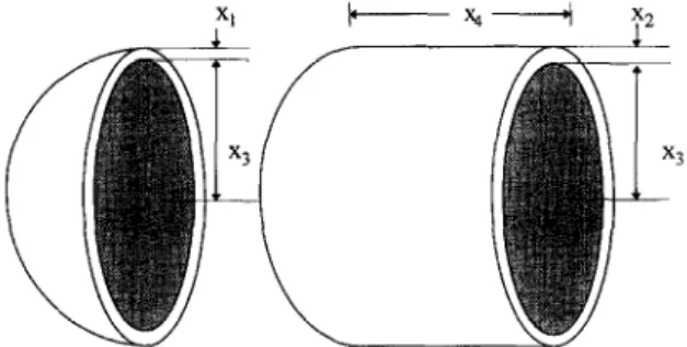
Example 2. Consider the optimal design problem of a pressure vessel in Sandgren [ 131 depicted in Fig. 1. Sandgren solved this problem by a Quadratic Integer

Programming Method, and Fu et al. [l] solved it by

an Integer Penalty method. Recently, Li and Chou

[9] solved this problem by the Multistart Method.

The problem is formulated below:

Min f(X) =0.6224x,x, + 1.7781x,x: 2 2 + 3.1661 x, xq + 19.84~~ xg subject to -x1 + 0.0193x, IO, -x2 + 0.00954x, IO, - nx;xq - +ITX; f 750.1728 I 0, -240+x,10, l.OOOIX, Il.375, 0.625 2 x2 2 1 .OOO,

Fig. I. Tube and end section of pressure vessel (from Sandgren [121X

where x, and x2 are discrete variables with discrete- ness 0.0625, and

47.5 5 x3 I 52.5, 90.00 I x4 I 112.00,

where x3 and x4 are continuous variables. x, is the

spherical head thickness, x2 is the shell thickness,

x3 is radius and xq is the length of the shell. Since x, and x2 are discrete variables, they can

be completely expressed by binary variables without

error, as shown below:

x1 = 1 + O.O625y,, + O.O125Oy,, + 0.2500~,~,

x2 = 0.625 + 0.0625~~~ + O.l25Oy,, + 0.2500y2,.

Suppose the tolerable error of approximating f( X >

(i.e. the objective function) is set as 0.05. Then we

can choose o3 = 0.34 and o, = 0.375. The variables x3 and x4 are then rewritten as

x3 = 47.50 + 0.34 y31 + 0.68 y32 + 1.36 Y,~ +2.72y,,+&,,

x4 = 90.00 + 0.375 y41 + 0.75 y,, + 1.5 y43 + 3 y44

+ 6~4, + 12~4, + ~4.

Table 1

A comparison of optimum solutions for Example 2

Items Optimal solution by

Sandgren’s method

Optimal solution by Fu et. al’s method

Optimal solution by the proposed method

Xl 1.125 1.125 1.000

*2 0.625 0.625 0.625

x3 48.95 48.38 51.25

106.72 111.745 90.991

(6)

630 H.-L. Li, C.-T. Gang/European Journal of Operational Research 107 (1998) 625-632

The maximal error of f(X) after linearization is

computed as

0.6224 1.7781

4 w36J4 + -w; 4 50.05.

Solving this program by LINDO [lo], the optimal solution is

x * = (1.000,0.625,51.252,90.991),

with objective function value f(X) = 7127.3. The

same problem was solved by Sandgren [13] and Fu

et al. [l]. The best solutions they can find, after

testing many starting points, are listed in Table 1. Table 1 shows that the proposed method can find a

solution better than the ones obtained by Sandgren

and Fu et al.

Example 3. To demonstrate the superiority of the

proposed method in finding the global optimum of

polynomial programs, several test examples of poly-

nomial programming problems listed in Hock and

Schittkowski [4] and Schittkowski [6] have been

evaluated. These examples have been solved by six

well-known optimization codes shown in Table 2.

Since none of these six codes could solve all test

problems successfully, and since none of them can

guarantee having found the global solution, Hock

and Schittkowski solved each test example by all of

these six codes. They executed each code with very

low stopping tolerances (10H7) and a huge amount

of starting points, thus computing one solution as

precise as possible. Only the best result obtained by

six codes is reported as the solution of the test

example.

The proposed method resolves these test examples

by setting the various tolerance values. The experi-

Table 2

Optimization programs for evaluating optimal solutions (Hock and Schittkowski [4]; Schittkowski [6])

Code Author Method

VF02AD Powell Quadratic approximation OPRQP Bartholomew-Biggs Quadratic approximation GRGA Abadie Generalized reduced gradient

VFOlA Fletcher Multiplier

FUNMIN Kraft Multiplier

FMIN Kraft, Lootsma Penalty

ment shows that the proposed method successfully

finds solutions for all test examples. Parts of the

results are listed in Table 3. The proposed method resolves each of these problems and finds the same or even a better solution than the best solution found by the other six codes. Take Problem 338 in [6] for

instance. The optimization problem is listed below:

(Problem 338 in [6])

Min F(X) = -(X:+X,2+X:)

subject to 0.5x,+x,+x3-1=0, x~+3x;+~x32-4=0,

where

X,

,

X,, X3 are unbounded.

The best solution of Problem 338 found by the six codes in Table 2 is

(X,, X,, X,> = (0.3669,2.244, - 1.427),

F(x) = - 7.2057.

in which the stopping tolerance is specified as 10V7 and a huge amount of starting points is tested.

We resolve this problem by specifying the toler-

ance as wi = w2 = w3 = 0.001 to obtain the solution

;“x x x1=(-

F(Y) =“‘- 10.993.

0.363659, - 1.66324,2.84507),

Solving this problem again by respecifying the toler-

ance as o, = o2 = w3 = 0.0001, we find the same

solution. Denote F(x * > as the value of objective

function for global optimum, the maximal error of

our solution with respect to F(x* >, is estimated

below referring to Proposition 2:

0.0001*

F(x) -F(Y) =3 4

i

)

G 10-8.

The obtained solution therefore is very close to the global optimum.

The comparison between these six codes and the

proposed method is discussed below:

The quality of the solution for these six codes

depends on the choice of starting point. In con-

trast, there is no requirement for the proposed

method to specify an initial point.

None of these six codes can guarantee having

found the global solution, but the proposed method

can ensure finding the global solution within a

(7)

Table 3 A comparison of optimum solutions found by the proposed method and six other codes listed in Table 2 Best solution by the other six codes Optimal solution by the proposed method X Objective value X Objective value 0- 1 variables No. of constraints Note F*(X) F*(X) Problem 2 1 in [4] (2.0) - 99.96 (2,O) - 99.96 12 91 * Problem 36 in [4] (20,11,15) - 3300 (20,11,15) -3300 34 I346 * Problem 37 in [4] (24,12,12) - 3456 (24.12.12) - 3456 34 1347 * Problem 44 in [4] (0.3.0.4) -15 (0.3.0.4) -1.5 40 326 * Problem 338 in [6] (0.336, 2.244, - 1.427) - 7.2057 (- 0.363659, - I .66324,2.84507) - 10.993 42 134 ** Problem 340 in [6] (0.6.0.3.0.3) - 0.054 (0.6,0.3,0.3) - 0.054 12 183 * Note: + = finds the same solution. * * = finds a better solution.

(8)

These six codes can only be applied to solving

problems with continuous variables. But the pro-

posed method can solve problems containing both

continuous and discrete variables.

Conclusions

This paper proposes a practical and useful lin-

earization technique to approximate polynomial terms

in a polynomial program. Using the technique, a

program with a polynomial objective function and

constraints can be solved to reach a global optimum

within a pre-specified tolerance. Many examples in

the literature are tested, which demonstrate that the

proposed method is very promising with regard to

solving a general polynomial program to obtain an

approximately global optimum.

Theoretically, the proposed method can solve a

polynomial program to find a solution which is as

close as possible to a global optimum. A major

difficulty of implementing the proposed method is

that if the range of a variable xi is large and the

upper bound of the tolerant error of xi (i.e., wi) is small, then it requires to add many binary variables

to represent xi. This will increase the computational

burden in the solution process. One possible way of

overcoming this difficulty is to divide the interval of

a variable before solving the problem. This remains for further study.

References

[I] Fu, J.F., et al., A mixed integer-discrete-continuous programming method and its application to engineering design optimization, Engineering Optimization 17 (1991) 263-280.

[21 [31 [41 [51 [61 171 [81 [91 [lOI [I11 [I21 [I31 iI41 [I51

Hansen, P., Jaumard, B., and Lu, S.H., A framework for algorithms in globally optimal design, ASME, Journal of

Mechanisms, Transmissions, and Automation in Design 1 I1 (1989) 353-360.

Hansen, P., Jaumard, B., and Lu, S.J., An Analytical approach to global optimization, Mathematical Programming

52 (1991) 227-254.

Hock, W., and Schittkowski, K., Test Examples for Nonlin- ear Programming Codes, Lecture Notes in Economics and

Mathematical Systems No. 18, Springer-Verlag. Heidelberg, 1981.

Hotst, R., and Tuy, H., Global Optimization: Deterministic

Approaches, Springer-Verlag, Berlin, 1990.

Schittkowski, K., More Test Examples for Nonlinear Pro- gramming Codes, Lecture Notes in Economics and Mathe-

matical Systems No. 282, Springer-Verlag. Heidelberg, 1987. Li, H.L., An approximate method for local optima for nonlinear mixed integer programming problems, Computers &

Operations Research 19/5 (1992) 435-444.

Li, H.L., A global approach for general O-1 fractional programming, European Journal of Operational Research 73 (1994) 590-596.

Li, H.L., and Chou, C.T., A global approach for nonlinear mixed discrete programming in design optimization, Engi-

neering Optimization 22 (1994) 1 G9- 122.

Linus, S., LINDO Release 5.3, LINDO System, Inc., 1994. Pardalos, P.M., and Rosen, J.B., Constrained Global Opti- mization: Algorithms and Application, Springer-Verlag,

Berlin, 1987.

Rinnooy Kan, A.H.G., and Timmer, G.. Towards global optimization methods (I and II), Mathematical Programming

39 (1987) 27-78.

Sandgren, E., Nonlinear integer and discrete programming in mechanical design optimization, Journal @Mechanical De-

sign 112 (1990) 223-229.

Sherali, H.D., and Adams, W.P., A hierarchy of relaxations between the continuous and convex hull representations for zero-one programming problems, SIAM Journal on Discrete Mathematics 3 (1990) 41 I-430.

Sherali, H., and Tuncbilek, C., A global optimization algorithm for polynomial programming problems using a reformulation-linearization technique, Journal of Global Opti-