Adaptive Feedforward Active Noise Cancellation in Ducts Using the Model
Matching of Wave Propagation Dynamics
Jwusheng Hu and Tesheng Hsiao
Abstract—Active noise cancellation in ducts using multiple
feedforward sensors have been investigated by many researchers. When adaptive algorithms were applied, usually a lumped pa-rameter model was assumed and the model includes the dynamics of the duct, sensors and actuators (e.g., microphone and loud-speaker). The distributed nature of the duct usually leads to a large parameter space and is difficult to implement direct adaptive control. This brief presents a control architecture which separates the duct’s dynamics from those of sensors and actuators. An adaptive control algorithm is proposed to cope with the unknown dynamics of sensors and actuators. Experiments were conducted to show the effectiveness of the control law.
Index Terms—Acoustic control, active noise control, adaptive
control, digital signal processor, distributed parameter system.
I. INTRODUCTION
A
CTIVE NOISE CANCELLATION (ANC) in ducts using feedforward sensors has been investigated for years [1]–[4]. This problem still receives considerable attentions in recent years [10]–[17]. In signal processing community, the research goal is to identify the dynamics of various sound transmission paths online in order to apply algorithms such as Filter-x LMS. To identify the secondary path between the control input to the error measurement, usually an auxiliary signal is added (independent of the noise source) to the control input [5]–[9]. Several proposals to enhance the performance such as the convergence speed were reported [10], [11], [14]. For narrow-band or tonal noise, earlier work by the authors [19] indicated that only phase information is needed for feedback cancellation. In recent years, frequency-domain based sub-band architecture was proposed to remove the need of secondary path modeling [15], [16]. The issues of slow convergence and large computational effort remain to be improved.The second issue occurs when there is no independent mea-surement available for the noise source. Hence, removing the influence of the actuator signals from the feedforward sensors’ measurement (called acoustic feedback) is a key to performance enhancement. The technique also requires an additive white noise signal generated online to identify the feedback path [13]. Several proposals to overcome the acoustic feedback were reported [17]. The adaptive feedback neutralization [18] is the
Manuscript received February 12, 2011; accepted July 05, 2011. Manuscript received in final form July 16, 2011. Date of publication August 30, 2011; date of current version June 28, 2012. Recommended by Associate Editor M. Guay. This work was supported in part by the National Science Council of Taiwan under Grant NSC 98-2622-E-009-190-CC2.
The authors are with the Department of Electrical Engineering, National Chiao Tung University, Hsinchu 30010, Taiwan (e-mail: [email protected]).
Digital Object Identifier 10.1109/TCST.2011.2162628
one mostly discussed in the signal processing related literature. The work in [17] proposed an adaptive noise cancellation (ADNC) filter to remove the influence of the reference signal. So far, no work on the scheduling of the additive noise power is reported and a rigorous proof of global convergence and stability is still lacking.
Despite the progress in the development of signal processing algorithms for ANC, very few considered the overall system control issues. One of the difficulties for ANC in ducts is that the plant is a distributed parameter dynamic system with a large number of poles and zeros. Common control engi-neering practice is to model the system via reduced-order state-space techniques and various control methods were ap-plied [24]–[27]. The methods have to deal with the controller design accuracy problem induced by a large order model. The term “feedforward” in ANC means to pick up the noise signal in space before it arrives at the actuator location. If the acoustic feedback exists, this creates an additional feedback loop. Canceling the feedback path by filtering is effective if the path model is known accurately [28], [29]. Another way of reducing the influence of the acoustic feedback is to use the wave propagation property. Based on the theory of acoustic circuit, an analytical solution for cancellation was derived using one upstream microphone [31]. Similar ideas were explored in [20]–[22] via control-oriented close-form plant model. The controller using two upstream microphones [20] also achieves cancellation by creating an infinite impedance boundary at the secondary source location. As shown in this work, the for-mulation of model matching gives the solution of all possible controllers for less-than-two upstream microphones. Further, the principle can also be applied to a dual actuator system [23]. In fact, sound wave propagation is essentially the same as the elastic extensional waves in solid. An interesting idea to stop the transmission of the extensional wave in one direction using two upstream sensors was reported [30].
In this work, the feedforward ANC problem from the per-spective of model matching under the closed form solution is developed. The advantage of the model matching formulation is that we can obtain a parameterization for all possible controllers that achieve the broad-band noise cancellation objective. An in-teresting observation is that all the controllers are also indepen-dent of the boundary conditions, similar to the one microphone solution by acoustic circuit [31]. Second, the model matching formulation also leads to a method of separating the duct’s dy-namics from the dydy-namics of sensor and actuator. As a result, an adaptive algorithm is proposed to identify the sensor and actu-ator dynamics online. Without the need to handle the distributed part of the plant, the length of the parameter vector in the adap-tation is greatly reduced. An experiment is conducted to verify the proposed methods.
II. MODELING ANDNOTATIONS
Consider a finite-length and hard-wall duct with two point
sources, (located at ) and (at ).
In the sequel, is called the primary source which may represent a disturbance input and is called the secondary source denoting a control input. For convenience, it is assumed that . Based on the notations defined in [21], the re-sponse of the system is written as (see Fig. 1): when
(2.1a) when (2.1b) and when (2.1c) where (2.1d) (2.1e) (2.1f) (2.1g) is the length of the duct and is the speed of sound. and are the boundary reflection coefficients at and
, respectively. The boundaries are assumed to be passive and the boundary reflection coefficients satisfy the following conditions.
Assumption 2.1: and .
In other words, under such assumption, the following charac-teristics have stable roots:
(2.2a) (2.2b) In practice, when feedback or feedforward control is applied, we need to consider the dynamics of loudspeaker and electronic
Fig. 1. Schematic diagram of the ANC system.
Fig. 2. Block diagram illustrating the model matching of feedforward ANC.
components. Let denote the controller’s output, the sec-ondary source can be modeled as
(2.3) where is the combined dynamics of sensor (micro-phone), actuator (speaker) and electronic components.
III. ADAPTIVEFEEDFORWARDCONTROLLAW
A. Model Matching Architecture
In this section, a general model-matching architecture using two feedforward sensors is presented. Consider a feedforward ANC system as shown in Fig. 1. Based on notations defined in Section II, an equivalent block diagram can be drawn as Fig. 2, where (3.1a) (3.1b) (3.1c) (3.1d) (3.1e)
All the transfer functions are related to the path dynamics in the ANC literature. represents the primary path, the secondary path, an the acoustic feedback paths and an the paths between the noise source and feedforward sensors. an are controllers to be de-termined.
Now it is easy to see that the downstream response can be represented as
(3.2a) Hence, for ideal broad-band noise cancellation (i.e.,
), the controller can be found by solving the following model matching formulation:
(3.2b) By substituting (2.1) and (3.1), it can be reduced to the following simple form:
(3.3) An interesting observation is that (3.3) does not depend on the boundary conditions. Obviously there are infinite sets of which satisfy (3.3). Assume that is invertible, the solution can be formulated as
(3.4a)
(3.4b) Equation (3.4a) and (3.4b) give a parameterized solution of all possible feedforward controllers that satisfy the cancellation ob-jective in Fig. 1. in (3.4a) and (3.4b) must be selected to satisfy the internal stability. Under Assumption 2.1, it is easy to verify that the stability requirement of Fig. 2 is the following transfer function vector is stable:
(3.5) A control law is proposed in [20] by assigning
which results in the following:
(3.6)
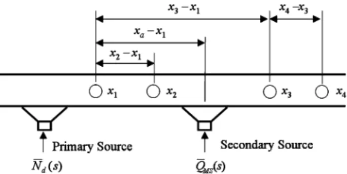
Fig. 3. Duct with four-sensor measurements.
Although the controller in (3.6) satisfies the cancellation con-straint of (3.3), it is not internally stable. Therefore, a modifi-cation of the controller to allow sacrifice in performance was proposed as [20]
(3.7) Further, the control law requires a perfect inversion of
which might be impossible in practice. Let denote a stable approximation of with a stable additive uncertainty
as
(3.8) As a result, the controller (3.6) is modified as
(3.9) The work in [20] proved that by properly selecting and making small enough, the overall system is stable.
B. Adaptive Control Law
As shown in the preceding section, the performance and sta-bility of the modified controller (3.9) depends on how accurate the inversion of [ in (3.9)] is. Further, aging ef-fect, temperature effect and so on will affect the characteristics of . Therefore, online adjustment of (the inverse approximation of ) becomes quite necessary. Before in-troducing the adaptive algorithm, an important relation among sensors in ducts (see Fig. 3) is observed first.
If , it can be shown that
(3.10)
where and
. The importance of (3.10) is that this relation not only separates the sensor-actuator dy-namics from the distributed system, but is also independent of the noise input (the primary source in Fig. 3). As a result, it serves as the equation for parameter identification. The idea of
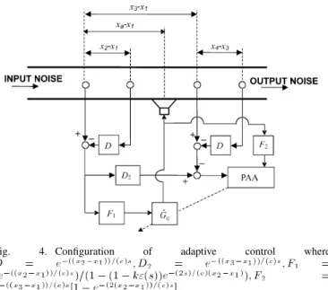
Fig. 4. Configuration of adaptive control where
D = e ; D = e ; F =
(e )=(1 0 (1 0 k"(s))e ); F =
e [1 0 e ].
using two pairs of microphones to separate forward and back-ward propagation waves was reported in [32]. The purpose is to identify the path dynamics for robust noise control that is insen-sitive to boundary conditions. This work shows another property of using two pairs of microphones as described above. Assume that there exists a causal and stable transfer function such that
(3.11) Applying (3.11) to (3.10), we have
(3.12) Let be the time domain signal of
and of ,
a parameter identification structure can be established as where denotes convolution (3.13) From (3.11), we can replace in (3.9) with . This results in the following equation:
(3.14) where is the time domain signal of
and of . Equation (3.13) is used to identify and (3.14) is the control action. Notice that contains a de-layed control signal . It means that the parameter adaptation process essentially find out the solution of that smoothes control signals in the past. Fig. 4 shows the adaptive control con-figuration.
The contribution of the novel adaptive structure is the dis-covery of (3.10) which removes the dependency of noise signals through a set of microphones. In the presence of noise signals, it is not easy to identify the I/O map online in this application be-cause the control signal is strongly related to those signals. Note that the feedback control action of (3.14), originated from (3.9),
is stable if the difference of to is
small (3.8). Therefore, if the convergent rate of the parameter identification of (3.13) is fast enough, the overall system is stable also. In practice, a short period of random signals can be injected into the system for identification before taking the control action to ensure the convergence.
IV. EXPERIMENTALRESULTS
An experiment was conducted to verify the feedforward con-trol law. The duct’s dimension is 18 cm 18 cm 200 cm and its cutoff frequency is about 945 Hz. A DSP-based system was used to perform real-time calculations and the sampling rate was chosen to be 5000 Hz. The loudspeaker’s diameter used in this experiment was 16 cm. The speaker is placed at 140 cm. Four microphones are mounted at 50.3 cm, 57.2 cm, 181.4 cm, and 188.3 cm. The arrangement of microphone and speaker locations is made such that the various delay terms in (3.12) can be approximated by integer delay in discrete domain. As a result, the discrete domain approximation of (3.12) is
(4.1) where is an approximation of . Let
(4.2) The time domain equation of (4.1) can be arranged into
(4.3) Equation (4.3) can be used as the equation for identification of . However, since we are only interested in identifying within the control bandwidth, it is necessary to limit the bandwidth of (4.3) to obtain a more accurate result. One way to perform this bandwidth-limited identification is to filter the control signal . But this filter must be zero-phase in order not to affect the phase of identified. In this experiment, we use a 50th order FIR band-pass filter and an extra 13-tap delay is added to ensure zero-phase. The final equation for identification becomes
(4.4) where is the FIR band-pass filter with passband of 100–900 Hz. The controller of (3.6) is approximated as
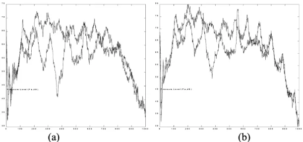
Fig. 5. Noise cancellation result: (a) open-ended downstream boundary, (b) downstream boundary half-covered by hard wall; blue line: noise, red line: after control.
To limit the control signals within the bandwidth, a 12-tap zero-phase band-pass filter is added to the left-hand side of (4.5), i.e.,
(4.6)
where . Let be an th order
FIR filter, i.e.,
Equation (4.4) can be parameterized as
(4.7)
where and
.
Simi-larly, the controller (4.6) can also be parameterized as
(4.8)
where and
. Equa-tion (4.7) and (4.8) are used as the parameter update and control signal, respectively. In the experiment, we choose and . The parameters were identified using a standard projection algorithm. Two types of boundary conditions at the downstream open end were tested. Fig. 5(a) shows the cancellation result when downstream boundary is open and Fig. 5(b) when downstream boundary half-covered by hard wall. A pseudo random noise is injected into the primary source in both experiments. These experiments show the effectiveness of the proposed algorithm in broadband noise reduction. The algorithm is robust under different boundary conditions. How-ever, at certain frequency range, the noise level is increased, especially in Fig. 5(b). Experimental experiences show that this could be caused by the inaccuracy of the simple delay
approximations in various part of the proposed algorithm (e.g., both microphone and speaker are not point sensor and source).
V. CONCLUSION
An adaptive control algorithm using two feedforward micro-phones in ducts is proposed in this brief. The control structure is designed such that the sensor and actuator dynamics are sep-arated from the acoustics. A four-microphone configuration is proposed to identify the sensor and actuator dynamics in the presence of noise and control actions. Experimental results are shown to demonstrate the effectiveness of the control law. It is shown that the adaptive controller is also robust under boundary condition changes.
REFERENCES
[1] M. L. Munjal and L. J. Eriksson, “Analysis of a linear one-dimensional active noise control system by means of block diagrams and transfer functions,” J. Sound Vibr., vol. 129, no. 3, pp. 443–455, 1989. [2] L. J. Errikson, M. J. Allie, and R. A. Greiner, “The selection and
ap-plication of an IIR filter for use in active sound attenuation,” IEEE
Trans. Acoust., Speech, Signal Process., vol. ASSP-35, pp. 433–437,
Apr. 1987.
[3] M. A. Swinbanks, “The active control of sound propagation in long ducts,” J. Sound Vibr., vol. 27, pp. 411–436, 1973.
[4] G. E. Warnaka, L. A. Poole, and J. Tichy, “Active Acoustic Attenua-tors,” U.S. Patent 4 473 906, Sep. 25, 1984.
[5] L. J. Eriksson and M. A. Allie, “Use of random noise for online trans-ducer estimate in an adaptive active attenuation system,” J. Acoust. Soc.
Amer., vol. 85, pp. 797–802, Feb. 1989.
[6] C. Bao, P. Sas, and H. Van Brussel, “Adaptive active control of noise in 3-D reverberant enclosures,” J. Sound Vibr., vol. 161, pp. 501–514, 1993.
[7] S. M. Kuo and D. Vijayan, “A secondary path estimate techniques for active noise control systems,” IEEE Trans. Speech Audio Process., vol. 5, pp. 374–377, Jul. 1997.
[8] M. Zhang, H. Lan, and W. Ser, “Cross-updated active noise control system with online secondary path modeling,” IEEE Trans. Speech
Audio Process., vol. 9, no. 5, pp. 598–602, 2001.
[9] M. Zhang, H. Lan, and W. Ser, “A robust online secondary path mod-eling method with auxiliary noise power scheduling strategy and norm constraint manipulation,” IEEE Trans. Speech Audio Process., vol. 11, no. 1, pp. 45–53, 2003.
[10] A. Carini and S. Malatini, “Optimal variable step-size NLMS algo-rithms with auxiliary noise power scheduling for feedforward active noise control,” IEEE Trans. Audio, Speech, Lang. Process., vol. 16, no. 8, pp. 1383–1395, 2008.
[11] J. Liu, Y. Xiao, J. Sun, and L. Xu, “Analysis of online secondary-path modeling with auxiliary noise scaled by residual noise signal,” IEEE
Trans. Audio, Speech, Lang. Process., vol. 18, no. 8, pp. 1978–1993,
Aug. 2010.
[12] X. Sun and S. M. Kuo, “Active narrowband noise control systems using cascading adaptive filters,” IEEE Trans. Audio, Speech, Lang. Process., vol. 15, no. 2, pp. 586–592, 2007.
[13] Y. Xiao, L. Ma, and K. Hasegawa, “Properties of FXLMS-based nar-rowband active noise control with online secondary-path modeling,”
IEEE Transactions on Signal Processing, vol. 57, no. 8, pp. 2931–2949,
Aug. 2009.
[14] M. T. Akhtar, M. Abe, and M. Kawamata, “A new variable step size LMS algorithm-based method for improved online secondary path modeling in active noise control systems,” IEEE Trans. Audio, Speech,
Lang. Process., vol. 14, no. 2, pp. 720–726, Feb. 2006.
[15] D. Zhou and V. A. DeBrunner, “New active noise control algorithm that requires no secondary path identification based on the SPR property,”
IEEE Trans. Signal Process., vol. 55, no. 5, pt. 1, pp. 1719–1729, May
2007.
[16] M. Wu, G. Chen, and X. Qiu, “An improved active noise control algorithm without secondary path identification based on the fre-quency-domain subband architecture,” IEEE Trans. Audio, Speech,
Lang. Process., vol. 16, no. 8, pp. 1409–1419, Aug. 2008.
[17] M. T. Akhtar, M. Abe, and M. Kawamata, “On active noise control systems with online acoustic feedback path modeling,” IEEE Trans.
Audio, Speech, Lang. Process., vol. 15, no. 2, pp. 593–600, Feb. 2007.
[18] S. M. Kuo and D. R. Morgan, “Active noise control: A tutorial review,”
Proc. IEEE, vol. 87, no. 6, pp. 943–975, Jun. 1999.
[19] J. S. Hu, “Active noise cancellation in ducts using internal model-based control algorithms,” IEEE Trans. Control Syst. Technol., vol. 4, no. 2, pp. 163–170, Mar. 1996.
[20] J. S. Hu and J. F. Lin, “Feedforward active noise controller in ducts without independent noise source measurements,” IEEE Trans. Control
Syst. Technol., vol. 8, no. 3, pp. 443–455, May 2000.
[21] J. S. Hu, “Active sound attenuation in finite-length ducts using close-form transfer function models,” ASME J. Dyn. Syst. Meas. Control, vol. 117, no. 2, pp. 143–154, 1995.
[22] J. Yuan, “Noninvasive model independent noise control with adaptive feedback cancellation,” in Advances in Acoustics and Vibration. New York: Hindawi Publishing, vol. 2008, Article ID 863603.
[23] D. Bismor, “Optimal and adaptive virtual unidirectional sound source in active noise control,” in Advances in Acoustics and Vibration. New York: Hindawi Publishing, vol. 2008, Article ID 647318.
[24] J. Hong, J. C. Akers, R. Venugopal, M.-N. Lee, A. G. Sparks, P. D. Washabaugh, and D. S. Bernstein, “Modeling, identification, and feed-back control of noise in an acoustic duct,” IEEE Trans. Control Syst.
Technol., vol. 4, no. 3, pp. 283–291, May 1996.
[25] A. J. Hull, C. J. Radcliffe, and S. C. Southward, “Global active noise control of a one-dimensional acoustic duct using feedback controller,”
ASME J. Dyn. Syst., Meas., Control, vol. 115, pp. 488–494, Sep. 1993.
[26] J. C. Carmona and V. M. Alvarado, “Active noise control of a duct using robust control theory,” IEEE Trans. Control Syst. Technol., vol. 8, no. 6, pp. 930–938, Nov. 2000.
[27] H. R. Pota and A. G. Kelkar, “Modeling and control of acoustic ducts,”
ASME Trans. J. Vibr. Acoust., vol. 123, no. 1, pp. 2–10, Jan. 2001.
[28] E. Esmailzadeh, A. Alasty, and A. R. Ohadi, “Hybrid active noise con-trol of a one-dimensional acoustic duct,” ASME Trans. J. Vibr. Acoust., vol. 124, no. 1, pp. 10–18, Jan. 2002.
[29] E. Esmailzadeh, A. Alasty, and A. R. Ohadi, “Multi-channel adaptive feedforward control of noise in an acoustic duct,” ASME J. Dyn. Syst.,
Meas., Control, vol. 126, no. 2, pp. 406–416, Jun. 2004.
[30] P. Naucler, B. Lundberg, and T. Söderström, “A mechanical wave diode: Using feedforward control for one-way transmission of elastic extensional waves,” IEEE Trans. Control Syst. Technol., vol. 15, no. 4, pp. 715–724, Jul. 2007.
[31] M. L. Munjal and L. J. Eriksson, “An analytical, one-dimensional, standing-wave model of a linear active noise control system in a duct,”
J. Acoust. Soc. Amer., vol. 84, no. 3, pp. 1086–1093, 1988.
[32] J. Y. Liu and K.-Y. Fung, “Robust active control of broadband noise in finite ducts,” J. Acoust. Soc. Amer., vol. 111, no. 6, pp. 2727–2734, Jun. 2002.