A sliding observer for nonlinear process control

(1)

Pergamon Chemical Engineering Science, Vol. 52, No. 5, pp. 787-805, 1997 Copyright 0 1997 Elsevm Science Ltd

A sliding observer for nonlinear process

control

Gow-Bin Wang, Sheng-Shiou Peng and Hsiao-Ping Huang*

Department of Chemical Engineering, National Taiwan University, Taipei, Taiwan, 10617,

R.O.C.

(Received 18 December 1995; in revised form 5 August 1996; accepted 12 September 1996)

Abstract-Sliding observers are considered as nonlinear state estimators with good robustness

to bounded modeling errors. In this paper we have developed sliding observers for process control. The observer is hence designed so as to possess invariant dynamic modes which can be

assigned independently to achieve the desired performance. Convergence of the estimating

algorithm is formulated by using Lyapunov stability theorems. Conditions for robustness to modeling errors are derived by analyzing the norms of estimation errors. For process control, servo-tracking and disturbance rejection for chemical reactors have been discussed by making use of this sliding observer. Simulation examples to demonstrate the construction and performance of this proposed sliding observer for chemical process control are also presented. 0 1997 Elsevier Science Ltd. All rights reserved

Keywords: Sliding mode; observer; observability; state estimation; nonlinear system.

1. INTRODUCTION

Various methods for designing nonlinear controllers have been reported in the literature. Unless they are

using ad hoc designs, most of the nonlinear controllers

such as those using feedback linearization (Hunt et a/.,

1983; Kravaris and Chung, 1987), GMC (Lee and Sullivan, 1988) and many others require the feedback of state variables to implement the control strategies. In practice, however, complete state feedback is im- practical in most applications. Although direct integration, i.e. open-loop observer, can be used to estimate the required state feedback and works well for a few applications, a closed-loop observer with feedback correction is still desirable, especially, when the system consists of modeling error(s) or pure integrator(s).

Although the theories and applications for linear systems are well developed, development of observers for nonlinear systems still provides an open area for research. Till now, development of observers for nonlinear systems has encountered many difficulties, such

as: requirement of extensive computational efforts,

coupling with controllers, uncertainty in the performance or robustness, restrictive conditions to be satisfied, etc. Some of the major difficulties encountered in the development of observers, which are reported in literature, have been reviewed by Misawa and Hed- rick (1989).

*Corresponding author.

In the last decade, attention has been focused on applying the transformed canonical forms for design (Bestle and Zeitz, 1983; Keller, 1987; Kantor, 1989;

Ding et al., 1990, etc.). For most of the nonlinear

systems, such a transformation can be defined

through Lie derivatives of the output which is a func-

tion of state variables (Gibon-Fargeot et al., 1994;

Alvarez-Ramirez, 1995). However, the resulting ca-

nonical forms are not strictly linear and the transformations thus involve exogenous inputs and a finite number of their derivatives. In case of simple systems, such difficulties involved in the transformations could be easily resolved. However, for systems having di- mensions greater than two, solution of the coordinate

transformations and existence of such transforma-

tions appear to be the bottleneck.

Recently, another type of observers that also use sliding mode have been reported. In the early work of

Slotine et al. (1987), the observer was constructed for

a second-order nonlinear dynamic system involving only single measurement. The extensions of such ob-

servers to nth-order and multi-output systems have

also been addressed in the literature. Further development in this field of sliding observer was made by

Misawa (1988). Canudas and Slotine (1991) have

further applied such observers in robot manipulators.

In all the studies mentioned above, a framework

similar to a Luenberger observer was used by appen-

ding a switching function with constant gains as

part of feedback corrections. To obtain such gains, different procedures have been proposed (Misawa and Hedrick, 1989). These procedures require certain 787

(2)

788 Gow-Bin Wang et al.

conditions to be satisfied or optimized with singular values which depend on the scaling factors. Thus, the procedures developed for determining the switching gains are complicated and the performance issue of the observers is also not addressed.

It is the purpose of the present paper to design sliding observers for control of nonlinear chemical processes. In chemical process control, measurements of indirect outputs are usually used to infer the key outputs which are rather difficult to be measured on-line. The sliding observer presented here is used to force these indirect but measurable outputs to lie on specified sliding surfaces, so that the resulting estimated states can be used to implement the nonlinear feedback control more efficiently. In order to design the observer independently, time-varying gains for the switching functions are used to keep the dynamic modes of these estimated states invariant regardless of the position of the states. For formulating the nominal convergence of the estimating algorithm, Lyapunov stability analysis has been used. Conditions for its robust stability are also derived herein. To demonstrate the potential use of this sliding observer, rejection of unknown disturbance by using a feedforward- like control is illustrated. Similar use for the model- based predictive control may be investigated in future research. Simulations for the application of chemical reactor control are given as illustrations for the potential uses of such sliding observers.

2. MATHEMATICAL FORMULATION

Consider a general nonlinear system as k = f(x, u)

Y =

h(x)

where x E R” is a vector of state variables, u E R” is the input vector and y E RP is the output vector.

To construct the nonlinear observers for the system given in eq. (1) it is essential to devise a correcting function @ such that, integration of the following equation would produce estimates of x, i.e. 9:

4 = f(%, II) + qy - 9)

(2) i = h(f).

3. SLIDING OBSERVER FOR SISO SYSTEMS

In the following text, for convenience, we shall use x, instead of z, to denote the state in eq. (3). Consider a SISO nonlinear system of the following form:

e = f(x, u)

(6)

Y = Xl

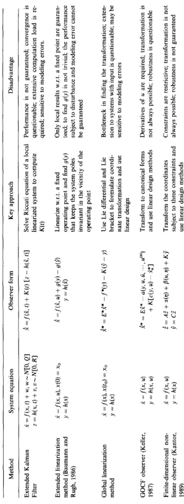
As has been mentioned earlier, many nonlinear observers have been reported in the literature. Although not exhaustive, various methods of approach along with their disadvantages for the few reported nonlinear observers are summarized in Table 1. To overcome some major obstacles in the construction of nonlinear observer for process control, a sliding observer is presented here.

where x = [x1 x2 ... x,IT is a state vector and u is an external input. The function f(x, u) in eq. (6) is subject to a norm-bounded modeling error.

The sliding observer for this SISO system becomes

ii =f,(ir, u) + k, sgn(x, - ai) i2 =f2(%, u) + k2 sgn(x, - a,)

(7)

We will assume that the Jacobian matrix of h, i.e.

J(h(x)), exists and is of full rank for all x E X, so that eq. (1) can now be transformed into the following system:

& =f,(%, u) + k,sgn(x, - x*i).

Let Pi = xi - Ti, i = 1,2, .‘. , n; then the above equation becomes

i = f*(z, u)

(3) y = cz

i?, = Afi + Sfi - kl sgn(Zi) ;, = Af2 +

Sf2

-

k2 sgn(Z,)

where C = [I, 0] and X is an open subset of R”. ;, = Afn +

6fn

-

k,sgn(x”,) Using eq. (3), z is partitioned into

so that an observer of the following form is constructed:

i = P(&, u) + K(t)a ₍₅₎

where K is a time-varying gain matrix and u is given as follows:

U=

swh - 9

wb2

-

9

i

wb,

f

-

&I

1

and the sign function, sgn(t), is defined as

i

1 ift>O sgn(t) =

- 1 if t < 0.

Further, let Z” = z“ - P lie on sliding surfaces by applying sliding conditions. The switching gain matrix, K, is formulated in order to keep the dynamic poles of Z* = z* - 4* invariant at desired constant values, which would lead to a good performance. Convergence of the estimating algorithm is formulated by using Lyapunov stability theorems and the robustness to modeling errors are derived via analysis of norms. Incorporation of such a sliding observer into a closed loop for process control is addressed in the following.

(3)

A sliding observer for nonlinear process control 789 where Afi =fi(x, U) -f;(%, u) and Sfi is the modeling

error due to structural deviation.

We can define a sliding function in terms of Z1 as s = 11

and a sliding condition for J, as either

(9)

or

$s = -qsgn(s) (11)

where q is a positive constant. In order to drive Z1 to its sliding surface, dZ,/dt should have a sign opposite

to that of fl. To do so, we can assign the value to kl as

kl >q+F. (12)

Here, we assume that the dynamic uncertainty is explicitly bounded, i.e.

IAfi + hfil G F (13)

where F is a positive constant. Thus, inequality (12) can make the variant trajectories point towards the surface s(t) = 0, where the tracking estimation error .C1 is zero.

Applying the concept of equivalent dynamics in accordance with Filippov (Slotine and Li, 1991), the convex combination of the dynamics on both sides of the surface s(t) leads to

i, = ;l(Af, + WI + k,) + (1 - y) (Afi + Sfi - k,)

.& = r(.G + ~~ + k2) + (1 - Y) (Afi + Sf2 - k,) (14)

;, = 1/(4fn + 6f + k,) + (1 - y) (A& +

Sfn

-

k,).

When k, is determined from eq. (12), we have

S = f, = 0, i.e.

dAf1 + WI + h) + (1 - Y) (Afi + Sfi - k,) = 0. Hence, the value of y is given as

h

-Afi -6fi y=

2kl (15)

Substituting eq. (15) into eq. (14) gives the reduced-

order sliding observer dynamics in the form of

.& = Afz + Sfz - Wkd (Afi + Sfd

$3 = Af3 + Sf3 - b’dkd (Afl + Sfd

(16) % = Afn + 6fn - Wk,) (Afl + Sfi).

By linearizing locally with respect to the point at %, eq. (16) can be treated as a state observer with the

following total differential form:

k, = {.$;g}& + . . . + {?&%&}i”

In the following, we first neglect the structural modeling error terms. Linearization is made on the basis of each point of the estimated states, instead of a fixed point of equilibrium, hence, the deviations considered for linearization are Zis, rather than considering how far they are away from the 6xed point. Consequently, this would be less restrictive compared to the extended linearization method of Baumann and Rugh (1986).

Let

k,

k, =

k,

[!

L X” where f, E R”-’ and H(k)4 af2 kz afi - --- ax, kt ax, af3 k afl - --- ax2 h ax2 afn km afi - _-- ax, k, ax, E R(“-1)X(“-1)

*

x2 _

1 i-1

= H(B) “.’ X”

(18)

7 af2 kz afl . ---- ax, h ax, af3 ks afl . . . ---- ax, h ax, afn kn afl ---- ax, _{h ax, 1} (19) To keep the eigenvalues of the observer invariant, the

switching gains, k,A [kz k3 ... kJT, can be directly

calculated by a specific formula depicted below. From eq. (19), it becomes

H(k)

=

- af2 af2 ax, “. dx, . : ai ’ i -ax, _{‘.’ ax, I} p v,f, - BV,,fl JA A, -

/?c,.

(20)

(4)

Method System equation Table 1. Evaluation of various nonlinear observers Observer form Key approach Disadvantage Extended Kalman Filter Extended linearization method (Baumann and Rugh, 1986) Global linearization method GOCF observer (Keller, 1987) Finite-dimensional nonlinear observer (Kantor, 1989) i=f(x,t)+w,w-N[O,Q] 2 =f(i, t) + K(t)

[z

-

h(i, c)] z=h(x,t)+u,u-N[O,R] .i =f(x, u), x(0) = xg i =fG, 4 + L?(Y) - s(P) Y =

w

y

=

h(Z) i =f(x), x(to) = xg i* = E*P* -f*(y) - K(j - y) Y =

w

i = f(x. u) Y = &, 4 i = j-(x, u) Y =

w

i* = Es* ~ a(y, u, li, ‘. ) d ”)) + KCC(Y, 4 - 21

z*

=

A.? + cc(q) + B(u, q) + KY j =

cz^

Solve Riccati equation of a local Performance is not guaranteed; convergence is 2 linearized system to compute questionable; extensive computation load is re- 6 K(r) quired; sensitive to modeling errors. f? % Linearize w.r.t. a fixed operating point and find g(y) that keeps the system poles invariant in the vicinity of the operating point Only local results w.r.t. a fixed point are guaranteed; to find g(v) is not trivial; the performance subject to disturbance and modeling error cannot be guaranteed Use Lie differential and Lie bracket to formulate coordinate transformation and use linear design Bottleneck in finding the transformation; exten- sion to systems with input is questionable; may be sensitive to modeling errors Transform to canonical forms Derivatives of u are required; transformation is and use linear design methods not always possible; robustness is questionable Transform the coordinates Constraints are restrictive; transformation is not subject to three constraints and always possible; robustness is not guaranteed use linear design methods

(5)

Observer with variable ?i = Ax + B(u + II) structure (Walcott and + f(C x) Zak, 1986) y = cx Sliding observer (Slotine et al., 1987) i =f(x, t) y =

cx

.i = A,? + Bu + Ky + S(t, i, y) f(t, u) = Pm ‘C ’h(t, x) Bc = P-‘C ’rw(t) S(t, i, y) = - P m ’C ’Ce/(llCell)p(t) PA0 + A;P = - Q 4 =f(<, t) - H(y - Cl?) - K w(F) Simple observer for input affine systems (Gauthier et al., 1992) 1 =f(x) + g(x) u Y = h(x) 2 =f(?) + g(P) u + S, ‘CT(y - CT) Observer for state affine systems (Gibon-Fargeot et al., 1994) i = A(w(t))x + h(w(t)) Y = h(x) i = A(w(t))i + b(w(t)) + S- ‘(t) x C ’(_Y - ca) Determine h(t, x) and find P and Q to form a Lyapunov equation; determine S(t, P, y) using VSS techniques Use sliding surfaces and constant switching gain K Transform coordinates and solve a Riccati equation Solve a Riccati equation to provide time-varying gains Bottleneck in finding P, Q and h(t, x); the way to lump nonlinear terms into f(f, x) is not unique; stability robustness is not guaranteed Positive realness may be too restrictive; performance is not guaranteed, extensive efforts in design procedure to guarantee robustness for bounded modeling errors. System should be of input affine; transformation be invertible; performance is not guaranteed; ro- * bustness to modeling errors is questionable E a System should be of state affine; performance and g convergence are not guaranteed; robustness to % modeling errors is questionable I 2

(6)

192 Gow-Bin Wang et al.

Let a,P[az a3 ... a,] be the coefficient vector of the Thus, if xi is in sliding mode, we would have k, = 0

characteristic equation of A,, i.e. and all the first time derivatives of li, i 2 2, will be

det(sI - A,) = s”-l + a2snm2 + a3.fA3 + ... + a, = 0.

given by eqs (8) and (16) so that

V-(Z)

= i,.k, +

‘.’ +

_;;k,

Also, define

=

MAfi + Sfz -

k2 sgn(?i)] + ..

Pi = [cl’ A,TC,T (A;)%; ... (A;)“-%:]-’

+

%CAf + K -

k,sgnGdl and

1

a2 1 0 1

.

. . ..oo . . 0 0

:I’

:

1

R, =

. .

an-2 an-3 ... 1 0 i = [cc2 2’3 “’ 2.1 a,_, a,_, “. a2 1

af2

kz

afl

af2

kz

afl

----

. ----

If a,A[cr2 ct3 ... cr.] is set to be the coefficient vector

ax2

h 3x2 ax. h ax, of the desired characteristic equation of H(B), then the

Bass-Gura formula (Kailath, 1980) can be used to

----

ah h ah

~. ----

af3 k3

afi

x2

derive the following:

ax2 h ax,

ax. h ax,

x3

X

flT =

(a, - a,) (R;

‘)TP1.

₍₂₁₎

Therefore, when the poles of the reduced-order sliding x kn

ah

ah k afl

[11

X”

----

observer are assigned, the designed switching gains

ax2

klaxz --lax, ax,

can be calculated as

k, = k,/I = k,PTR; ‘(a, - a,)T. ₍₂₂₎

Furthermore, to eliminate undesirable chattering

effect, it is practical to replace the sign function in

eq. (7) by a saturation function, sat(s/$), which is

defined as

sat(s/4) = {

44 if

Is/4 <

1

sgn(W if Is/4 I > 1. (23)

It is clear that by using the sliding condition for the It has been shown that the switching gains,

state corresponding to the measured output, state ki, 2 < i < n, are calculated according to eq. (22),

xi is forced to lie on a sliding surface. As a result, the hence enabling matrix H(%) to have specific eigen-

reduced-order observer has invariant dynamic poles values in the LHP. Therefore, the stability of the

and is guaranteed to converge asymptotically. On the reduced-order observer for nominal case, i.e. 6f = 0,

other hand, it should be noted that this approach can be guaranteed.

would inevitably introduce tracking error. Hence, The issue of robustness of the observer concerns

a trade-off between tracking accuracy and control whether or not x^, diverges in the presence of modeling

power has to be achieved by suitably choosing the errors. From eqs (17) and (25), it can be defined that

boundary layer thickness 4 (Slotine and Sastry, 1983). _{i, = H(f)%, +}_6,

4. NOMINAL CONVERGENCE AND ROBUSTNESS Further, the solution for .C7, can be expressed as

Substituting xi, corresponding to the measured

s

,

output, onto a defined sliding surface, we further show r7, = eH’$(0) + eHctmr)S, dr. (26)

that even for the remaining states the observer is 0

stable and is robust to modeling errors. _{If il%,(O)/I < a and there exist}_{b, e}_{and N such that}

Let the Lyapunov function I/ be of the form

II afll G @ + Ne-“‘Ml + II k, II/k,)

(27)

V(1) = !{2’: + 2; + .‘. +

n;}.

₍₂₄₎

then we have Then we have

b N --E*

(7)

A sliding observer for nonlinear process control 793

where -A,,, (i., > 0) represents the greatest eigenvalue of H(f), I/ ?& 11 is the vector norm of 8, and a, b,

N and E are all positive constants. The derivation of

eq. (28) is given in the Appendix. It may hence be concluded that

(i) iii,/1 would remain bounded, if (/Sf(l Q (h + Ne-“‘)/(l + likJ/kl), b > 0 and 0 < F: < i,.

(ii) l/%,(1 + 0. if h = 0, 116f(l d (Ne-“Ml + llk,ll!k,) and 0 < c < i,,.

In other words, the estimation errors of the reduced- order observer remain bounded if //6f /I is bounded as given in eq. (27).

5. SLIDING OBSERVERS FOR MULTI-OUTPUT SYSTEMS

For multi-output systems, the construction of sliding observer can be derived directly from the SISO system by approximately the same way as described above. Nevertheless, the method of finding switching gain matrix K would require more sophisticated mathematical manipulations. For process control, however, we are more interested in formulating the problem as follows.

Instead of using a full matrix, we assign a block diagonal form to K in eq. (5). In other words, we can renumber the system and divide the system into sev- eral subsystems. Within each subsystem, the state estimations are corrected by a sign function based on the same output. The key issue would be the assign- ment of each pivot switching gain that would keep the output on its sliding surface, and the reduced-order system to have invariant dynamic modes. We will illustrate these procedures by using a system which has two outputs. First, according to the system

k = f(x, u) y = cx we can renumber the states such that

Partition the vector x into x0 and xb, so that

? = [a, b* “’ z&J

i* = [,?, &+I “’ .<.]‘.

The observer is then formulated as follows:

2 = f”(P, S*, u) + k” sgn(y, - .cl) i* = f*(P. B*, u) + k* sgn(y( - a,) where (29) (30) k” = [k, k2 ... k,_JT and kh=[kpk,+, ... k.]‘. Thus, we can assign two sliding surfaces as

.Sl = .?I and s2 = X,.

The resulting reduced-order system now becomes

where

k; = [k2 k3 .‘. k,-,I’ and kf = [k,+, k,+, ..’ Therefore, we have a reduced observer pair as

knl

r.

and K. as

(33)

We can further derive k’: and k,b from the following equality:

detjsl - A, + K,C,} = n (S - ni)

i=l (34)

where ii, i = 1,2, ... , n - 2, are the specified eigen- values. Solving eq. (34) for deriving kz and k! would need tedious algebraic manipulations if n is higher than three. Chen (1984) has provided three effective methods to find K,.

Although there may be different ways of partitioning the observer into the subsystems as given in eq. (30), however, there is little change in the reduced- order system given in eq. (31) except for the changes in configuration of K, matrix. Hence, different decompo- sitions would result in the same set of columns for the observability matrix of [A,, C,] pair. The changes in the system due to different partitioning of subsystems are in fact changes in the eigenvectors of (A, - K,C,) which are associated with each dynamic mode (Chen, 1984; Lewis, 1992).

While formulating the observer for chemical processes, wherein state variables can obviously be classified into non-interacting groups, we can take advantage of this method of partitioning. Thus, eq. (30) becomes

in = f”(P”, II) + k”sgn(yl - 2,)

i* = f”(i”. S*, u) + k* sgn(y, - $). (35) Hence, we shall have

(8)

194 Gow-Bin Wang et al.

Fig. 1. The serial CSTR system.

In other words, the computations for k: and kg can

now be decoupled. Each of the k: and kf can be calculated individually by using eq. (22) for each of the subsystems. In the following, we will illustrate this proposed sliding observer with an example of estimation of a chemical reaction system.

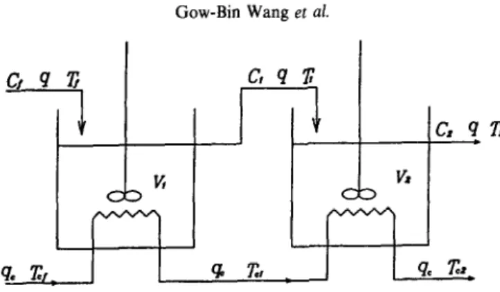
Example (State estimationfor a serial chemical re-

action system): Figure 1 shows the serial continuous- stirred tank reactor (CSTR) system, belonging to the multi-output case and studied by Henson and Seborg (1990). The dynamic behavior of this system can be governed by the following equations:

Cl = +(C,

-

Cl)

-

koCl exp 1 ( > - g 1 T~=+(T,- T1)+ (- ~WOCl exp E ( > -- 1 PC, RTI +O.Olu[l -exp(-%)1(7,1-x4 it3 = x1 - x3 - kOx,exp

It is apparent that this reacting system has two

measurable outputs, i.e. it can be split into two subsystems. Therefore, to estimate the concentrations in the reactor, one can design the sliding observer as follows:

+ k1 sgn(Z,/$)

C?,

= $(Cl

-

C,)

-

koCz exp (37)

The nominal values of the parameters of this serial CSTR system are given in Table 2. The state variables x, system output y and manipulated input u are defined as follows:

x&CC1 T1 C2 T21T, yp[T1 T2 T ) upq,.

Hence, the dynamic model of the serial CSTR in dimensionless form gives

i1 = 1 -x1 -koxlexp

4, =

T, - XI2 +

k”(- AH)

i,exp

( >

- -$

+o.olu[l -:+Jii:- a,)

+

k2

sgnGdd4

+ k3 sgn(W4) (39)

where &g x4 - &. The switching gains kz and k4 are

determined according to eq. (12). The other two

switching gains can be directly calculated according to eq. (22).

(9)

A sliding observer for nonlinear process control 795 Table 2. Nominal parameter values for the

serial CSTR system

where X is an open subset of R”. The operator M is defined as

Variable Nominal value

M'hi(X,

U) = hi(X)

4 v, = v,

C f

T/ T cf k, E/R (- AH) P = I', cp = c PC u/4, = UA, 100 l/min 1001 1 mol/l 350 K 350 K 7.2 x 10” min- ’ 10,000 K 4.78 x lo4 J/mol 1000 g/l 0.239 J/g K 1.67 x lo5 J/min K M’hi(X, U) = T [f(X, u)] Mkhi(x, u) =

&M*-‘hi(x,

u)

1 T

f(x, u)

^I

T + g M’-‘hi(X, U)

1

i ₍₄₂₎

For this simulation case, the process input is given as

1

90 l/mm if 0 < t < 5 min

u=

100 l/min if t > 5 min. (40)

Initial conditions for the true states and the estimated

states are set as CO.085 442 0.005 4501T and

CO.05 442 0 4501T, respectively, and the switching

gains of the measurable outputs are set as k2 = 80 and

k4 = 25. A suitable boundary layer thickness $J = 0.01

is also selected. It is apparent that the values of species

concentrations should either be positive or zero.

Hence, when the estimated concentration values, i.e.

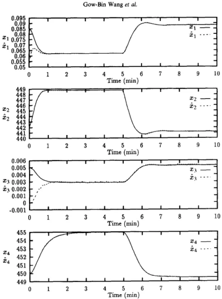
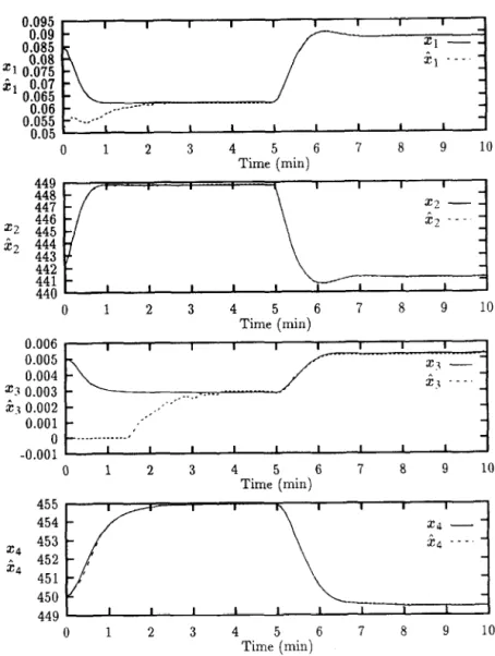
ii and i3, are lower than zero, they are set to be zeros. Estimation results, which are depicted in Figs 2 and 3, demonstrate the performance of the proposed sliding observer for state estimations.

6. APPLICATION TO PROCESS CONTROL The sliding observers developed in the previous section offer advantages such as: ease of construction

and on-line implementation, robustness to modeling

errors and guaranteed convergence. However, prior to applying such an observer to process control, two issues need to be resolved. One is the observability of states in the closed-loop and other is the stability after combination.

For the former, consider a nonlinear system as

given in eq. (I), its local observability at x E X depends

on whether the following condition is satisfied (Keller, 1987): ran1

la

>

T \% M” - ‘h(x, u) wherei=1,2 ,..., pandk=1,2 ,..., n.

It can be clearly seen that the rank of this observability matrix would be a function of x and u. For open loop use, the values of u can be freely assigned. Nevertheless, in closed-loop control, it is important to note that the control inputs are no longer free variables. However, since u cannot be explicitly separated from x, it becomes difficult to determine whether it is feasible to construct an observer for closed-loop control under certain feedback law.

A simplified expression for local observability condition at each local point of (x, u) can be given for non-affine systems as follows:

Rank

The above condition is a direct result of the assump- tion that at (x, u) the system is locally observable and hence the system can be locally linearized by using the PBH rank test. To construct an observer for closed- loop control, it is however necessary to examine the observability condition of eq. (41) over a domain of x as well as that of feasible control input.

Some special cases having simpler observability condition are as follows:

Input afJine systems: A large number of dynamic processes have the system equations in form of

x = f(x) + g(x)u

y = h(x).

(44)

For such systems, a sufficient condition for local observability at some x0 E X would be to find n independent row vectors among the following (Vidyasagar, 1993):

=n ₍₄₁

(10)

796 Gow-Bin Wang et al. :lik_-_::r 0 1 2 3 4 5 6 7 8 9 10 Time (min) ~~~~ t@-y+yy 0 1 2 3 4 5 6 7 8 9 10 Time (min)

Fig. 2. Estimation results of the serial CSTR system under sliding observer with observer poles

Pm = Pm = - 5.

As the vector u does not explicitly appear in the above governed by the following equations:

formulation, to construct an observer for closed-loop

system, it would be required to examine the observ- % = f(x, u)

ability condition over a given domain of x only. _{P =}_{f(2, u) + cD(y - j)} ₍₄₇₎

State afine systems: For some chemical reaction y = cx

systems (Gibon-Fargeot et al., 1994), the dynamic where @ designates a correcting function which is

equations can be described by the following equa- _{used in the observer. If we define the difference be-}

tions: tween the true states and the estimated states as

g = W(r)* YW + b(e), Y(t))

(46)

2=x-f

y = cx. then the above governing equations become

The observability, for this kind of systems, would ir = f(x, u)

depend on whether or not the (A, c) pair is observable. (48)

The other criterion to be considered while using the P = f(x, u) - f($ u) - (D&i).

observer for nonlinear process control is whether in- In linear systems, it is easy to show that 12 and x have

corporation of the proposed sliding observer into independent dynamic modes, and the dynamic modes

a control system would cause only stability problem. of the overall system would be a combination of both

To answer this question, we shall consider a general sets. Thus, incorporating a stable observer into

(11)

Fig. 3. Estimation results of the serial CSTR system under sliding observer with observer poles

PO1 = PO2 = - 2.

the formulation of a stable closed-loop system. In Moreover, within the neighborhood of some equilib- general, it is difficult to reach such a conclusion for rium point x0, we can further derive that

nonlinear systems. However, it is essential to know that, if the estimated states converge asymptotically to

their true values with bounded transient errors, then i=f(x”.u(xo))+(“,f+~~)~~=~(x-x,l whether a stable state feedback system remains stable

after incorporating the proposed sliding observer. + W(xo,2)(x - x0) + o(i? (51) According to the result given in the previous sec-

tion, eq. (48) for the system that uses the proposed ^

sliding observer now becomes =Z V,f,, .\,] +Ee Sui?x \_1” + W(x,, 2) _>(x -- xg)

(49) _where

(50)

W(xo> ~,~V,(Q(xF) = Vxq, Iy z x0% + V,q, Ix = x,.G It can be obviously seen from eq. (50) that g7, is

independent of x. On the other hand, eq. (49) can be + “’ + vxq”I.=.,~” linearized with respect to 2 at the point of i = 0, i.e.

P = x, as and

i = f(x, u(x - 2)) = f(x, u(x)) + E ; _ = 1 + o(2).

x cl

Q(x)+; _~ = cw) 9b4 ... m)i. (52)

(12)

798 Gow-Bin Wang et al. Let A(x,,1)~V,fJ.=., +:g _ + W(x,, 3 x - 7.” I (53) p ‘4(x,) + W(x0, 5). where Al(xa, 0) = ,4(x,).

The local stability of this system can be guaranteed by studying the eigenvalues of the following linearized matrix at the equilibrium point x0:

A(x,, %) = ,4(x,) + W(xo, 2).

It is known that, without loss of generality, one can set x0 as 0. Thus, we have

A(0,

2) = A(0) + W(0, 2).

Notice that the ideal system, whose all states are accessible, is stable such that all the eigenvalues of A(0) lie in the LHP. The effect of the observer on its stability is limited to the extra term, W(O,r?). The

stability of this observer-based closed-loop system

should be discussed in light of the following theorem. Theorem (Perturbation theorem for the eigenvalue,

Stewart and Sun, 1990): Let 3, be a simple eigenvalue of

the matrix A, with right and left eigenvectors v and w,

and let A = A + E be a perturbation of A. Then there

exists a unique eigenvalue 1 of .& such that

X=n+ _gHyoHEv _{+ o(llEl12)}

Based on the above theorem, we have

X[A] =

)*[A] -z ₊

_{4l Wl12). (55)}

We can therefore conclude that if

oHWv

max 7

il I

< I~il Vi

WV

the incorporation of this sliding observer would not

affect its nominal stability which is derived from the ideal system. As can be seen from eq. (51), as f ap- proaches zero as time passes, the observer based system will convert to an ideal system.

Although the stability of such an observer-based system cannot be said to be totally independent of the observer, the stability condition can be achieved more easily since this sliding observer provides the guaranteed convergence as in the previous analysis. As a result, if the control using full state feedback is globally stable within a defined domain of x, it should be possible to incorporate a carefully designed observer which will not cause a stability problem. Conse- quently, design of the state feedback control and the

observer can be implemented separately. In other

words, one can design a stable control system by assuming that all state variables are fed back. A sliding observer as depicted above can then be constructed. Following this guideline, we illustrate in the following subsections the use of such a sliding observer for controlling chemical processes.

6.1. Setpoint tracking of chemical reactor control

It is known that all control systems are nonlinear to a certain extent. Hence, the development and applica-

tion of nonlinear control algorithms are attracting

great attention in the recent years. Here, we utilize the GLC structure to deal with the servo control problem of an isothermal CSTR. The GLC approach was first proposed by Kravaris and Chung (1987) for obtaining the linear relationship between the transformed inputs and process outputs for nonlinear systems (Bequette, 1991). Therefore, the linear control theory, which is well-developed for the linear systems, can be utilized to complete the controller design.

For a minimum phase nonlinear system with rela-

tive order r, the state feedback control law

u= v - Ljh(x) L,Lj- ‘h(x)

can directly transform the original nonlinear system into

y”’ = a. ₍₅₈₎

Furthermore, the new manipulated input v is set to be r = - #gJ- 1) _ tj_ry”-2’

- _- _02Y _- _Qlb _- _Ys,). ₍₅₉₎

The closed-loop transfer function (CLTF) of the system can then be obtained by combining eqs (58) and (59) as

Y(S) Ql

-=

ys,(s) s’ +

t&s’-’ +

“’ +

e,s +

e1

(60)

It may be mentioned here that most of the nonlinear control techniques utilize state feedback compensator

laws. Hence, the employment of state observers

becomes necessary. In the following, we solve the estimation and control problems of the chemical reaction system by applying the sliding observer developed above.

Let us consider a well-mixed CSTR with isothermal reaction as

A=B+C.

By denoting the concentrations of species A, B and

C as xi, x2 and x3, respectively, material balances for this CSTR are described by the following dimensionless equations: iii = 1 - xi - &Xi + D,4 & = Dlxl - x2 - D2xf - D3x: + u i3 = D3x: - x3 y = h(x) = x3. (61)

(13)

Since the system has relative order r = 2, according to in form of

eqs (58) and (59), we have

P, = 1 - x^l - DlzZl + D& + kl sat&/+)

j;=v= _{- &J; - Hl(Y -} _YJ ₍₆₂₎ _{$2 = DIP1 - 22 -}_{D& - D& + u + k2}

sat(Z,/4)

Then the corresponding nonlinear control law de-

rived from eq. (57) gives 23 = D3x*$ - g3 + k3 sat&/$) (65)

U= - 2D,~,(D,P, - i2 - D$;) + (D$; - y) - fQD$; - y) - Bl(y - y,,)

2D,.u*, (63)

where f31 and e2 are tuning parameters of the GLC where & = x 3 - 2, and the switching gains are deter-

approach. The overall closed-loop transfer function is mined from eqs (12) and (22).

thus obtained from eq. (60) as During the simulations, we choose the process

Y(S) 01 parameters as D, = 3, D2 = 0.5 and D3 = 1 and set

-=

Y,&) sz + 02s + 81’ (64) the initial conditions of the true states x(O) and the

estimated states $0) as CO.356 0.921 0.8481T and

Furthermore, the estimated values of the unmeasur- [0.5 1.0 0.8481T, respectively. Two tuning parameters

able states, $I and &, in the nonlinear control law, i.e. of the GLC approach are placed at @I = 4 and e2 = 4.

eq. (63), are provided by the proposed sliding observer In this study, the control objective is to make the

0.1 0.05 0 51 -0.05 -0.1 -0.15 I I I I I I I I I ..‘-I_, “... po1 = po2 = -4.0 - C....

“‘A JJO] = po2 = -1.5 ..’ -

--_ I I I I I 1 I I I 0 1 2 3 4 5 6 7 8 9 10 Dimensionless Time - pfJ1 = po2 = -4.0 - po1 = po2 = -1.5 ” ” - x2 -0.1 - -0.12 I .:’ -0.14 2, : -0.16 - ‘.,,_ j” -0.18 ” ’ I I I I I I I I 0 1 2 3 4 5 6 7 8 9 10 Dimensionless Time v ‘V ._ ._ 1 I I _-. ._-_ _. po1 = po2 = -4.0 - po1 = po2 = -1.5 ‘... - ._ zcz -0.0015 ; ; -0.002 -‘: ,-- - .- _{_} -0.0025 - ’ I I I I I I I I 0 1 2 3 4 5 6 7 8 9 10 Dimensionless Time

Fig. 4. Results of estimation errors for the isothermal CSTR system under sliding observer with observer poles pal = poz = - 4 and - 1.5.

(14)

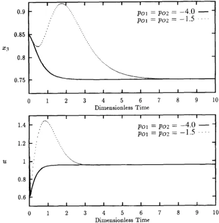
800 Gow-Bin Wang et al. dimensionless concentration x3 track its setpoint

y,, = 0.75 as soon as possible. Let the switching gain

k3 = 1.5 and the boundary layer thickness C$ = 0.01.

From the results of estimation errors shown in Fig. 4, it is clear that the unmeasurable concentrations can be effectively estimated by the proposed sliding observer. The servo control responses shown in Fig. 5 demonstrate the tracking performance of this sliding observer. Furthermore, it may be noted that the assigned poles of the reduced-order sliding observer do influence the convergence rate for state estimation.

Moreover, when the modeling errors occur due to parametric uncertainty, the proposed sliding observer can still perform well by setting this parameter as an unknown state variable.

6.2. Disturbance rejectionfor chemical reactor control The presence of unknown disturbance in the process would prevent fi from converging to zero. As a result, the estimated states deviate from their true values which, in turn, would degrade the control performance. One way to reject such unknown disturbance is to include it in the observer as an extra state variable. For constant disturbance, this extra state serves as an integrator, i.e. for SISO systems, we have

states, xZr . . ..x.+,, including the unknown disturbance.

The matrix that corresponds to H(%) in eq. (19) would now become

~*(%,.-&+I) =

V&f, -

Bcvx,fll

V++,f, -

Bcvx”+,fi1

- *

CVJI

1 - IcIcvx”+,fil

₁. (67)

The existence of parameter sets of p and $ of such a system would depend on the observability pair (A*, c*) of the following nature:

A* = [

Vx,f,

VX”

+ ,

fr

0 1 xcn- 1) ₀_{1X1 1}

’

(68)

c* =

CVx,h

vr”+,.fil.

If the pair (VJl, V,,f,) is observable, a necessary and sufficient condition for this augmented system to be observable is

k =f(x,x,+1 = 44, ~,+,=O, .v=x1 (66)

Equation (69) is a result of applying the observability where d is an unknown disturbance. A sliding ob- condition (Morari and Stephanopoulos, 1980) to server can be constructed to estimate the unmeasured the (A*, c*) pair. For multi-output systems, the

0.9 0.85 XR 0.8 :- I I I I I I I .’ ‘.. .’ ‘.,, _{po1 = po2 = -4.0} _- _- po1 = po2 = -1.5 “” . . . . .._ ‘..._ _{‘.._} 0 1 2 3 4 5 6 7 8 9 10 Dimensionless Time I I I I 1 I I I I 1.4 _ ,?...,, po1 = po2 = -4.0 - - po1 =po2 = -1.5 “” 1.2 - : ‘....( u

I

I I I I I I I I I I 0 1 2 3 4 5 6 7 8 9 10 Dimensionless Time

Fig. 5. Servo control responses of the isothermal CSTR system under sliding observer with observer poles pOl = p02 = -4 and - 1.5.

(15)

A sliding observer for nonlinear process control 801 number of unknown disturbances to be included in an

observer is at the most equal to the number of system outputs.

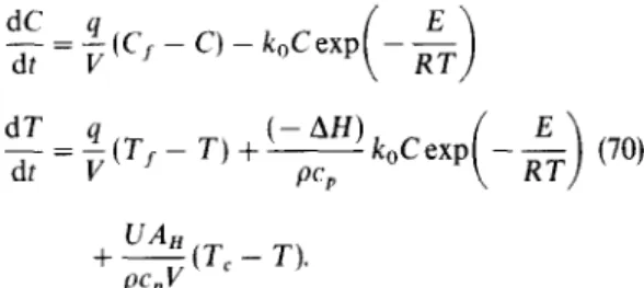
In the following example, we consider a well-mixed CSTR with first-order, irreversible, exothermic reaction. Material and energy balances for such exothermic CSTR are described by

dC q

- =

v (C, - C) - k&exp dt

+~(Tc-

n

where C and T represent the reactant exit concentration and reactor temperature, respectively. Let the four im-

portant dimensionless parameters be denoted as

D = koVemD” bP q ’ D 7 = (- AfW,oD, PC,Tf (71)

The corresponding dimensionless variables are de-

fined as C x1 =-) T - T,

CfO

x2=-

T,

D 4, dl

cc,, ,+

CfO

Tc - T,

(72) u = ~ D4D5, Tf y = c, J’,,, = T

where d, represents the unknown disturbance and

Cfo is the nominal value of the feed composition. After introducing the dimensionless quantities given

0.025 , _I 0.02 0.015 0.01 0.005 0 po1 = po2 = -4.0 - po1 = po2 = -1.5 “.’ - open-loop observer - k. “... ‘.. --..I__ I I I I I 0 1 2 3 4 5 6 7 8 9 10 Dimensionless Time 0.03 , I I I 1 I I I r 1 _I pal = pox = -4.0 - PO] =po2 = -1.5 ‘.. open-loop observer - -0.03 1 I I I I I I I I I I 0 1 2 3 4 5 6 7 8 9 10 Dimensionless Time I I I I I 1 I I I po1 = po2 = -4.0 - po1 = po2 = -1.5 “’ open-loop observer - ‘... ‘X. L -k. I -$--.__J I I I I I 0 1 2 3 4 5 6 7 8 9 10 Dimensionless Time

Fig. 6. Results of estimation errors for the exothermic CSTR system under sliding observer with observer poles pal = po2 = - 4 and - 1.5 and under the open-loop observer.

(16)

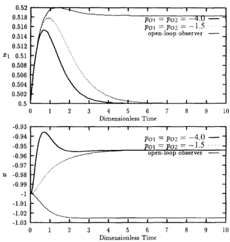
802 Gow-Bin Wang et al. PC?1 = PO2 = -4.u - - PO] =po2= -1.5 - open-loop observer - 0 1 2 3 4 5 6 7 8 9 10 Dimensionless Time -0.93 I I I I I I I I I po1 = po2 = -4.0 - - po1 = PO.2 = -1.5 - open-loop observer - -1.03 L I I I I I I I I I 0 1 2 3 4 5 6 7 8 9 10 Dimensionless Time

Fig. 7. Results of disturbance rejection of the exothermic CSTR system under sliding observer with observer poles po, = poz = - 4 and - 1.5 and under the open-loop observer.

above, the resulting normalized model is governed as where y, is the system measurement and

f*(x) = x3 - x1 - D,s~w(, +z2,D,)

Y = Xl> ym=x2.

In this case, the unknown disturbance dl is regarded as another state variable. According to eq. (73), we have

1,

=x3--,

-D6s,exp(l

+~,D,)efl(x)

We may now apply the GLC structure to solve the concentration control problem of the exothermic CSTR. The relative order r of this CSTR is equal to 2;

thus, let

ji=v= _- _{@2J; -} _{B,(Y - Ysp).} ₍₇₆₎ Then the corresponding nonlinear control law can be directly derived from eqs (74) and (76):

u=

(‘3, -

1 - D6

evCy,lU +

~,lD,)l~f,(~) -

{D64U +

ym/D4

IF2

wCy,JU +

**~,dJD,)l)f~(x*)**

+

@A4 -

Y,,)

D,W +

y,/D,)~ZewCy,lU

+

~,lD,)l

(77)

i2=D6D,x,exp(l+~2,D,)-(l+D,)xl+u

where O1 and B2 are tuning parameters of the GLC approach. The overall closed-loop transfer function (74) can be obtained directly from eq. (76) as

&f,(x) + 92w

Y(S) 4

-zz

(17)

Furthermore, the estimated values of the unmeasur- no requirement of canonical transformation, achieve-

able states, i1 and &, in the nonlinear control law, ment of desired performance by allocating the ob-

given by eq. (77), are provided by the proposed sliding server poles, knowledge of convergence and robust-

observer in form of ness of the estimation to the designer, etc. Potential

(1 +$o,)

uses of this sliding observer towards servo-tracking

4, = ?3 - ?I - DbPl exp + kl sat&/41 and disturbance rejection for process control are dis-

cussed. Estimation of unmeasurable states and con-

trol of chemical reactor are illustrated.

&=D,W,exp(l +tl,D,)-(l +D5)i2 _{Acknowledgement}

(79) Financial support from the National Science Council of

+ u + k2 sat&/$) the Republic of China(NSC-84-2214-E002-036) is gratefully

acknowledged.

j3 = +

k3 sat(ZZ/4).

where Z2 = x2 - z?~ and the switching gains are determined from eqs (12) and (22).

For comparisons, an open-loop observer is used to estimate the unmeasurable states by directly integrat- ing the following differential equations:

For the exothermic CSTR, the four process para-

meters in eq. (71) are chosen as D4 = 5, D5 = 0.5,

D6 = 1 and D7 = 2. Initial conditions for the true

states x(0) and the estimated states a(O) are set as CO.5 0 1.051T and CO.5 0 l.OIT, respectively. It should be noted that, in this example, the control objective is

to make the dimensionless concentration x1 remain

on its setpoint ysp = 0.5 in the face of the unknown disturbance. By applying the GLC approach, the two tuning parameters are set as o1 = 4 and e2 = 4. Fur-

ther, the switching gain k2 and the boundary layer

thickness 4 are set to be 1.5 and 0.01, respectively. Figure 6 reveals the existence of offset for estimation of the states for load change since the open-loop observer cannot provide correct estimated states. On the other hand, the response results shown in Fig. 7 demonstrate good robustness features of the reduced- order sliding observer in face of existence of an unknown disturbance.

7. CONCLUDING REMARKS

A sliding observer, which behaves like a reduced- order observer, is presented. This observer has been shown to overcome some major difficulties involved in constructing nonlinear observers for state estima-

tions, especially for nonlinear process control. To

achieve this, the switching gains in the observer are made to be time-varying. Convergence of the estimation is analyzed by using Lyapunov stability theorems. Robustness conditions, which would guarantee the observer to have a bounded error norm when facing modeling error, are also derived. The advantages of this proposed sliding observer include: simple and less restrictive design and construction, no need of extensive computations during its implementation,

R R R” R, sat sgn T u u V VW

a, b

AI, A2r -41 A, A”(x,, 3 CP Cl. C c, d DI-D7 E f, g F

Af

h H(k) AH J ko K L M N PO19 PO2 Pl NOTATION positive constants heat transfer area

matrix in eq. (20) or eq. (32) matrix in eq. (53) heat capacity vector in eq. (20) concentration matrix in eq. (32) disturbance

process parameters of the reaction system

activation energy

vectors of nonlinear functions positive constant defined as f(x, u) - f(f, u) output functions matrix in eq. (19) heat of reaction Jacobian matrix

specific reaction rate constant time-varying gain matrix Lie operator

operator defined in eq. (42) positive constant

poles of the reduced-order sliding ob-

server

inverse of the transpose of the observability matrix of [A,, c,] pair

feed flow rate matrix in eq. (52) relative order ideal gas constant real scalar field

n-dimensional real vector field

lower triangular Toeplitz matrix with

first column [l a2”. an_2 a,_,]

sliding surface saturation function sign function time temperature input vector

overall heat transfer coefficient transformed control variable reactor volume

(18)

804 Gow-Bin Wang et al.

W(x,, 2) defined as V,(Q(x) %) Kailath, T. (1980) Linear Systems. Prentice-Hall,

X state vector Englewood Cliffs, NJ, U.S.A.

Y output vector Kantor, J. C. (1989) A finite dimensional nonlinear Ym measured output observer for an exothermic stirred-tank reactor.

2 state vector Chem. Engng sci. 44, 1503-1510.

Keller, H. (1987) Non-linear observer design by trans-

Greek letters formation _{form. Int. J.}into a generalized _{Control 46, 1915-1930.}observer canonical

a 4 [XI c!s ” cr”]

B vector defined in eq. (20)

Kravaris, C. and Chung, C. B. (1987) Nonlinear state feedback synthesis by global input/output lineariz- Y coefficient in eq. (15) ation. A.1.Ch.E. J. 33, 592-603.

bf

modeling error due to structural devi- Lee, P. L. and Sullivan, G. R. (1988) Generic

ation model control (GMC). Comput. Chem. Engng 12,

& vector defined in eq. (25) 573-580.

1 positive constant Lewis, F. L. (1992) Applied Optimal Control and Es- ;

positive constant timation. Prentice-Hall, Englewood Cliffs, NJ, tuning parameters of the GLC approach U.S.A.

eigenvalues Meditch, J. S. and Hostetter, G. H. (1974) Observers

A _{for systems with unknown} _{and inaccessible} _inputs.

V vector _Int._{J. Control 19, 473-480.}

P density _{Misawa, E. A. (1988) Nonlinear} _{state estimation} _using d vector defined in eq. (5) sliding observers. Ph.D. thesis, Massachusetts Insti- @ correcting function in eqs (2) and (47) tute of Technology, Cambridge, U.S.A.

;

boundary layer thickness Misawa, E. A. and Hedrick, J. K. (1989) Nonlinear positive constant observers - a state-of-the-art survey. ASME J.

w vector Dyn. System Measurement Control 111, 344-352.

Morari, M. and Stephanopoulos, G. (1980) Part II:

Subscripts structural aspects and the synthesis of alter-

r reduced-order system native _232-246.feasible control schemes. A.I.Ch.E. J. 26,

Superscripts *

estimated value deviation value

REFERENCES

Alvarez-Ramirez, J. (1995) Observers for a class of continuous tank reactors via temperature measurement. Chem. Engng Sci. 50, 1393-1399.

Baumann, W. T. and Rugh, W. J. (1986) Feedback control of nonlinear systems by extended linearization. IEEE Trans. Automat. Control AC-31,

40-46.

Bequette, B. W. (1991) Nonlinear control of chemical processes: a review. Ind. Engng Chem. Res. 30, 1391-1413.

Bestle, D. and Zeitz, M. (1983) Canonical form observer design for non-linear time-variable systems.

Int. J. Control 38, 419-431.

Canudas de Wit, C. and Slotine, J.-J. E. (1991) Sliding observer for robot manipulators. Automatica 27,

859-864.

Chen, C. T. (1984) Linear System Theory and Design.

Slotine, J.-J. E., Hedrick, J. K. and Misawa, E. A. (1987) On sliding observers for nonlinear systems.

ASME J. Dyn. System Measurement Control 109, 245-252.

Slotine, J.-J. E. and Li, W. (1991) Applied Nonlinear

Control. Prentice-Hall, Inc., Englewood Cliffs, NJ,

U.S.A.

Slotine, J.-J. E. and Sastry, S. S. (1983) Tracking control of nonlinear systems using sliding surfaces with application to robot manipulators. Int. J. Control

38,465-492.

Stewart, G. W. and Sun, J. G. (1993) Matrix Perturba-

tion Theory. Academic Press, San Diego, U.S.A.

Vidyasagar, M. (1993) Nonlinear Systems Analysis. Prentice-Hall, Englewood Cliffs, NJ, U.S.A.

APPENDIX A: DERIVATIONS FOR EQ. (28) From eq. (17), we have

k, = Hi, + 6,. (Al) Thus, we can solve that

i, = eHV,(0) + eHcrmr) S, dz. WI

Holt, Rinehart and Winston, New Y&k, U.S.A.

Ding, X., Frank, P. M. and Guo, L. (1990) Nonlinear Let 11 H,(O) )/ < a; we have observer design via an extended observer canonical

form. Systems Control Lett. 15, 313-322. _{ll?,l/ < a/leH’/l + rIJeH(r-rJII}_{IIS,lI dr} Gibon-Fargeot, A. M., Hammouri, H. and Celle, F. s 0

(1994) Nonlinear observers for chemical reactors.

Chem. Engng Sci. 49, 2287-2300. c ae -&,f +

I ‘em”&” /,a,,1 & (A3)

Henson, M. A. and Seborg, D. E. (I 990) Input-output 0 linearization of general nonlinear processes.

A.I.Ch.E. J. 36, 1753-1757. where - 1, (1, > 0) is the greatest eigenvalue of H(t). From

Hunt. L. R.. Su. R. and Mever. G. (1983) Global

eqs (20), (22) and (25), it is known that

,, \ I

transformations of nonlinear systems. IEEE Trans.

(19)

A sliding observer for nonlinear process control ₈₀₅ Then it can be derived that

116,II < IlSfJ +F Ilkrll < 116f/J Therefore, if there exist h: N and E such that

=ae-“m’+JL(l -e-“my+

‘%i . (A5)

[, _ e-‘“m-“l]

IIWI G (b + Ne-VI + lIk,ll/%)

where h, N and E are all positive constants and E < i,,, we shall obtain

h N

< ue-““I’ + _ +_e-“’

i. --E (A@

4n m

Hence, it is proved that /Ii, 11 is bounded. I( %,I1 < ae-“m’ + e-“m’

A sliding observer for nonlinear process control