RZ-DPSK調變技術在長距離光纖傳輸系統裡的理論探討及實驗

全文

(1)⊕ 國立中山大學光電工程研究所碩士論文. RZ-DPSK 調變技術在長距離光纖傳輸系統裡的理論探討及實驗 A Study of RZ-DPSK Modulation Scheme upon Long-haul Optical Fiber Transmission System. 研究生：許勝軒撰指導教授：多賀秀德. 中華民國九十七年六月.

(2) Master Thesis A Study of RZ-DPSK Modulation Scheme upon Long-haul Optical Fiber Transmission System ◎ Acknowledgments ……………………………………………II. ◎. 中文摘要…..………………..…. ………………………..III. ◎ ◎. Abstract…………………………………………………...IV List of Contents……………………………………………V. Chapter 1 Introduction 1.1 Background of long-haul optical fiber communication system……………………………………………………………1 1.2 Motivation of this Thesis………………………………………...1 1.3 Structure of this Thesis…………………………………………..2 Chapter 2 Theoretical study of the dispersion map upon the transmission performance of the long-haul RZ-DPSK system…… 2.1 Explanation of the simulation model……………………………4 2.1.1 Simulation model………………………………………....4 2.1.2 Simulation scheme………………………………………...6 2.1.3 Dispersion map…………………………………………..14 2.2 Comparison of the dispersion maps…………………………… 2.2.1 Effects of the SPM and the XPM………………………..17 2.2.2 Effects of the repeater output power…………………….19 2.2.3 Discussions………………………………………………22 Chapter 3 Experimental study of the transmission performance of the long-haul RZ-DPSK system 3.1 Introduction…………………………………………………...25 3.2 Experimental setup……………………………………………25 3.2.1 Transmitter………………………………………………26 3.2.2 Transmission Line……………………………………….27 3.2.3 Operation of recirlating fiber loop…. …………………..29 3.2.4 Receiver…………………………………………………31 3.3 Measurement of the transmission performance……………….32 3.3.1 Performance dependence upon the repeater output power.33 I.

(3) 3.3.2 Performance for different wavelength after 5000km transmission……………………………………….......36 3.3.3 Experimental investigation of the effect of the XPM….36 3.3.4 Experimental investigation of the effect of the SPM…..39 3.4 Discussions…………………………………………………….42. Chapter 4 Conclusion………………………………………………………...43 List of Abbreviation..........................................................................................45. II.

(4) 致謝這篇論文的完成，最重要的首先要感謝我的指導教授多賀秀德教授。在碩士的兩年期間，經由他的指導之下，讓我對於整個光纖通訊系統的原理以及實驗架構，都有了完整的基礎以及經驗；並且在這段時間之內，學習如何的架設整個實驗，並分析及量測所得到的實驗結果，最後整理成我們所需要的結論。這讓我在以後的工作領域上，有更顯著的幫助。除了指導教授之外，另外要感謝的就是我的碩士班同學吳俊億。經由他的協助，讓我在遇到問題的時候，可以有很清晰的解答。由於我們是第一屆的研究生，如果沒有他的大力協助老師，整個實驗室的建設可能不會這麼的順利。在研究所的兩年生活裡，學弟李建霖、林彥廷、陳睿軒、黃博灝、以及博士班學長王心民，也幫忙分擔了很多實驗室的其他事情，讓二年級的我們可以專心於論文的撰寫之上。此外，經由大家的相處之下，讓我在各個方面也有了不同的體驗，並學習到了看待事物的不同想法。最後，也是最重要的是感謝我的父母。如果沒有他們在背後支持我並且栽培我，是沒有辦法順利的考上研究所並順利畢業。謹以此論文獻給他們來向他們敬上最深的致謝。. 許勝軒 2008.06 III. 于西子灣.

(5) 中文簡介在現今的世界裡，長距離光纖通訊系統是一個非常重要的建設來支持最新的寬頻通訊。歸零碼差分相移鍵調變(RZ-DPSK)，在現在吸引了更多的注意歸因於其改善了長距離傳輸的增益表現，而去了解這種技術來改善系統的傳輸增益也是非常重要的。在目前的長距離光纖傳輸系統當中，色散圖是一項非常重要的技術，並且也廣泛的使用在世界各地的海底光纖傳輸系統當中。就現今而言，一種全新地，而且完全不同於以往已使用在海底光纖通訊系統當中的色散圖已經被發表出來，並展現出了對於長距離 RZ-DPSK 傳輸增益的提升。儘管如此，改善增益的原因尚未完全的証實；而這也是我們必須非常重要的探討並釐清增益改善在整個物理實驗上的機制，因為這將提供在不久之後，改進整個長距離光纖通訊系統的系統設計的可能性。在這篇論文當中，我們可以學習到在長距離 RZ-DPDK 傳輸系統當中的增益表現。包括了電腦上的模擬以及實作上的實驗，並且以這兩種所得出的結果來驗證在長距離 RZ-DSPK 傳輸系統當中不同因素對於傳輸增益的影響。從理論上，我們得知了自我相位調變(SPM)在傳統色散圖中，扮演了明顯的角色衰減整體的傳輸增益；但在新的色散圖中，這並沒有造成明顯的增益衰減。此觀察到的現象將會用實際上的實驗來驗證得知。. IV.

(6) Abstract Long-haul optical fiber communication system is an important infrastructure to support the latest broadband communication in the world. It is important to study a technology to improve the performance of such system, and the Return-to-Zero Differential Phase Shift Keying (RZ-DPSK) modulation attracts much attention because of its improved long distance transmission performance. One important technology of the current long-haul optical fiber communication system is the dispersion map, and it is widely deployed for already installed undersea optical fiber communication system in the world. Recently, a new dispersion map that was totally different from the map used for already deployed system was proposed, and it demonstrated advantageous performance of the long-haul RZ-DPSK transmission. Even though, the reason of the performance improvement is not investigated, and it is important to clarify the physical mechanism of the performance improvement, because it will contribute to improve the system design of the long-haul optical fiber communication systems in near future. In this master thesis, the performance of the RZ-DPSK format in the long-haul transmission system is studied. Both computer simulations and experiments are conducted to confirm the effects of various factors in the long-haul RZ-DPSK transmission system. From the theoretical study, it is pointed out that the Self-Phase Modulation (SPM) played a significant role to degrade the transmission performance of the conventional map, while it does not cause so significant degradation in the new map. The effects of the SPM and the Cross-Phase Modulation (XPM) with the conventional map are investigated through the experimental study.. V.

(7) Chapter 1 Introduction 1.1 Background of long-haul optical fiber communication The communication requires a transfer of the information from one point to another. If we want to convey the information over any distance, the communication system is required. In recent years, the internet communication system is using an electrical coaxial cable, but there are several disadvantages of electrical coaxial cable. They are a bandwidth limitation, an electromagnetic interference from space, etc. To support the growth of the internet traffic, the optical fiber communication system becomes more popular now, because the optical fiber communication system has the broad bandwidth. The research of the optical fiber communication system started around 1975, and the technology is widely deployed in the commercial communication system now. The optical fiber communication system has several advantages. (1) It has abilities to carry much more information and to deliver it with greater fidelity than either copper wire or coaxial cable. (2) It can support much higher data rates with longer distances than coaxial cable. This feature makes it ideal for transmission of serial digital data. (3) It has a low transmission loss that is 0.4dB/km for 1.3μm wavelength and 0.25dB/km for 1.5μm wavelength. (4) Since the carrier in the optical fiber is a lightwave and there is an optical amplifier, there is no need to use the opto-electrical converter to transform the signal in the middle of the transmission line. All optical system reduces the cost of the optical fiber communication system, especially the long-haul system. Long-haul optical fiber communication system is an important infrastructure to support the latest broadband communication in the world. As the Wavelength Division Multiplexing (WDM) technique is compatible to the all optical system, it is widely used in the long-haul optical fiber communication system. Current emphasis of the WDM lightwave system is to increase the system capacity by transmitting more and more signal wavelengths through the WDM technique. Nowadays, the long-haul optical fiber communication system is applied for over several thousands kilometers, and it is very useful for the commercial undersea communication system around the whole world.. 1.2 Motivation of this study Even though the optical fiber communication system has a superior transmission performance, current technology is not enough to support the faster growth of 1.

(8) undersea transmission traffic today. Recently, the Return to Zero Differential Phase Shift Keying (RZ-DPSK) modulation format is attracting more attention because of its improved transmission performance, and it realized a long-haul transmission system with extended repeater spacing [1-3]. One important point to note is that the design of the dispersion map of the RZ-DPSK system becomes significantly different from that of the conventional system using Intensity Modulation Direct Detection (IM-DD) [4]. Recently, a new dispersion map was proposed, and it demonstrated advantageous performance of the long-haul RZ-DPSK transmission compared to the conventional map that suited for the IM-DD based system [5]. As the conventional dispersion map is widely deployed for the long-haul undersea optical fiber communication system [6], it is quite stimulating to investigate the reason why the new dispersion map has the better transmission performance for the RZ-DPSK system. In this master thesis, the transmission performance of the long-haul RZ-DPSK system is investigated using the numerical simulation and the experiment. The difference of the transmission performance between the conventional map and the new map is studied through the numerical simulation. The transmission performance of the long-haul RZ-DPSK system is experimentally evaluated, and the effects of the Self Phase Modulation (SPM) and the Cross Phase Modulation (XPM) are investigated. Finally, appropriateness of the theoretical study is confirmed through the experimental result.. 1.3 Structure of this thesis There are 4 chapters in this master thesis. Chapter 1 is the introduction. This chapter explains the background and the motivation of this thesis. Numerical simulation study is described in chapter 2. In chapter 2, the numerical simulation using split-step Fourier method is conducted for the different dispersion maps of the RZ-DPSK system. The optical fiber nonlinear effects upon the transmission performance are also discussed. For chapter 3, the experiments are conducted to confirm the simulation results. The experiments show the 5000km transmission performance of the long-haul RZ-DPSK optical fiber communication. The numerical simulation results and the experimental results are compared and discussed. Finally, in chapter 4, this master thesis is concluded.. 2.

(9) References in this chapter [1] T. Inoue, K. Ishida, T. Tokura, E. Shibano, H. Taga, K.Shimizu, K. Goto, and. K. Motoshima, “ 150km repeater span transmission experiment over 9000km ” in proc. of 30th European Conference on Optical Communication (ECOC), paper Th4.1.3, Sweden, 2004. [2] J.-X. Cai, M. Nissov, W. Anderson, M. Vaa, C. R. Davidson, D. G. Foursa, L. Liu, Y. Cai, A. J. Lucero, W. W. Patterson, P. C. Corbett, A. N. Pilipetskii, and N. S. Bergano, “Long-haul 40 Gb/s RZ-DPSK transmission with long repeater spacing,” in proc. of Optical Fiber Communication conference (OFC) 2006, paper OFD3, Anaheim, 2006. [3] C. Rasmussen, T. Fjelde, J. Bennike, F. Liu; S. Dey, B. Mikkelsen, P. Mamyshev, P. Serbe, P. van der Wagt, Y. Akasaka, D. Harris, D. Gapontsev, V. Ivshin, and P. Reeves-Hall, “DWDM 40G transmission over trans-pacific distance (10 000 km) using CSRZ-DPSK, enhanced FEC, and all-Raman-amplified 100-km UltraWave fiber spans,” IEEE J. of Lightwave Technol., vol.22, no.1, pp.203-207, Jan. 2004. [4] M. Vaa, E. A. Golovchenko, G. Mohs, W. Patterson, and A. Pillipetskii, “Dense. WDM RZ-DPSK transmission over transoceanic distances without use of periodic dispersion management,” in proc. of 30th European Conference on Optical Communication (ECOC), paper Th4.4.4, Sweden, 2004. [5] G. Mohs, W. T. Anderson, E. A and Golovchenko, “A new dispersion map for undersea optical communication systems,” in proc. of Optical Fiber Communication conference (OFC) 2007, paper JThA41, Anaheim, 2007. [6] N. S. Bergano, “Wavelength division multiplexing in long-haul transoceanic transmission systems,” IEEE J. of Lightwave Technol., vol.23, no.12, pp.4125-4139, 2004.. 3.

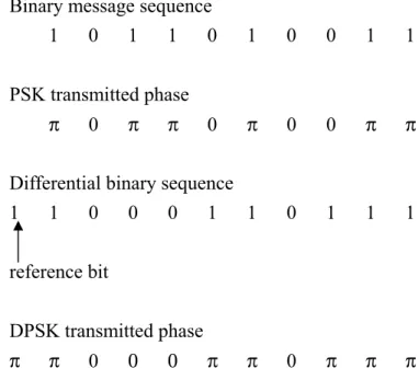
(10) Chapter 2 Theoretical study of the dispersion map upon the transmission performance of the long-haul RZ-DPSK system 2.1 Explanation of the simulation model Before conducting an experiment, the transmission performance of the DPSK format had been confirmed in numerical simulation. In this chapter, the explanation of the RZ-DPSK system and the simulation method to confirm the transmission performance for both the conventional dispersion map and the new dispersion map is discussed. The optical fiber nonlinear effects (the SPM and the XPM) cause the different effect to the performance of the long-haul RZ-DPSK system using the different dispersion map. Therefore, these effects are discussed using both dispersion maps in this chapter.. 2.1.1 DPSK format In the case of the PSK format, the optical bit stream is generated by modulating the phase φs in the next equation [1, 2]. Es (t ) = As (t ) cos [ω0t + φs (t ) ]. Here, Es is the electrical field of the signal light, As is the amplitude of the electrical field, and ω0 is the frequency of the optical carrier. They are kept constant when the phase φs is modulated. For binary PSK, the phase φs takes two values, commonly chosen to be 0 and π. An interesting aspect of the PSK format is that the optical intensity remains constant during all bits because the amplitude As is constant, and the signal appears to have CW form. Coherent detection is necessary for the PSK as the phase information is lost if the optical signal is directly detected. The DPSK is a derivative form of the PSK since the information is encoded as a change (or an absence of a change) in the optical phase on a bit by bit basis. The relationship between the DPSK and the PSK is illustrated in Figure 2.1. The PSK transmit the digital bit sequence as it is, while the DPSK transmit the sequence after encoding. The encoding is to compare the bit with the prior bit, and if these two bits are the same, “1” is generated as an encoded bit, while “0” is generated when these two bits are different. Hence the technique does not require phase comparisons over 4.

(11) more than two bit intervals, it relaxes the constraints of the PSK like a stringent requirement of the phase stability of the light source. In addition, the DPSK is a technique straightforward to implement at high transmission rates because the phase fluctuation between the two signal bits is reduced. Binary message sequence 1 0 1 1 0. 1. 0. 0. 1. 1. π. 0. 0. π. π. Differential binary sequence 1 1 0 0 0 1 1. 0. 1. 1. 1. 0. π. π. π. PSK transmitted phase π. 0. π. π. 0. reference bit DPSK transmitted phase π. π. 0. 0. 0. π. π. Figure 2.1 Comparison of PSK sequence and DPSK sequence The implementation of the PSK requires an external modulator capable of changing the optical phase in response to an applied voltage. The physical mechanism used by such modulators is called electrorefraction. Any electro-optic crystal with proper orientation can be used for the phase modulation. A LiNbO3 crystal is commonly used in practice. The design of LiNbO3-based phase modulator is much simpler than that of an amplitude modulator as a Mach-Zehnder interferometer is no longer needed, and a single waveguide can be used. The phase shift δφ occurring while the CW signal passes through the waveguide is related to the index change δn by the simple relation. δφ = (2π / λ )(δ n)lm where lm is the length over which index change is induced by the applied voltage. The index change δn is proportional to the applied voltage, which is chosen such that δφ = π. Thus, a phase shift of π can be imposed on the optical carrier by applying the required voltage for the duration of each “1” bit. In the case of the DPSK, information is coded by using the phase difference between two neighboring bits. For instance, if φk represents the phase of the kth bit, 5.

(12) the phase difference Δφ = φk – φk-1 is changed by π or 0, depending on whether kth bit is 1 or 0 bit. The advantage of the DPSK is that the transmitted signal can be demodulated successfully as long as the carrier phase remains relatively stable over a duration of two bits.. 2.1.2 Numerical method The Nonlinear Schrödinger (NLS) equation is a nonlinear partial differential equation that can not be solved analytically in general except for some specific cases in which the inverse scattering method can be employed. To understand the nonlinear effects in optical fibers using the NLS equation, a numerical approach is necessary in usual. There are many numerical methods that have been developed for this purpose. In this thesis, we used the split-step Fourier method, one method that has been used extensively to solve the pulse-propagation problem in the nonlinear dispersive media. To understand the split-step Fourier method, it is required to understand the wave equation and the pulse-propagation equation [3]. 2.1.2.1 Wave equation In this section we derive the pulse-propagation equation. The starting point is the wave equation ∇×∇×E = −. 1 ∂ 2E ∂2P − μ 0 c 2 ∂t 2 ∂t 2. (2.1.1). where E is the electrical field vector, μ0 is the vacuum permeability, ε0 is the vacuum permittivity, c is the speed of light in vacuum and the relation μ0ε0 = 1/c2 was used. Here, P is the induced polarization by E. In general, P and E is related using χ as P = χ (1) E + χ (2) E2 + χ (3) E3 + …. (2.1.2). In optical fiber case, due to the symmetry of molecule, χ(2) is 0. Then, P can be divided into the linear term and the nonlinear term as follows. P = PL + PNL. (2.1.3). PL and PNL are related to the electrical field by the following relations. ∞. PL (r, t ) = ε 0 ∫ χ (1) (t − t ') ⋅ E(r, t ')dt ' −∞. PNL (r, t ) = ε 0 ∫. ∞. ∫ ∫χ. (3). (2.1.4). (t − t1 , t − t2 , t − t3 )E(r, t1 )E(r, t2 )E(r, t3 ) dt1dt2 dt3. −∞. 6.

(13) (2.1.5) Then, from the Maxwell’s equation, ∇ ⋅ D = 0 and a × (b × c) = b(a ⋅ c) − (a ⋅ b)c , eq.(2.1.1) can be re-written as:. ∇ × ∇ × E = ∇(∇ ⋅ E) − ∇ 2 E = −∇ 2 E. (2.1.6). By using these equations, equation (2.1.1) finally can be re-written in the form. ∇ 2E −. ∂ 2 PNL ∂ 2 PL 1 ∂ 2E = + μ μ 0 0 ∂t 2 ∂t 2 c 2 ∂t 2. (2.1.7). where the linear and the nonlinear parts of the induced polarization are related to the electric field E(r,t) through equations. (2.1.4) and (2.1.5), respectively. 2.1.2.2 Nonlinear pulse propagation. To solve the equation (2.1.7), it is necessary to make several simplifying assumptions. First, PNL is treated as a small perturbation to PL. Second, the optical field is assumed to maintain its polarization along the fiber length so that a scalar approach is valid. Third, the optical field is assumed to be quasi-monochromatic. The last assumption is valid for the pulses as short as 0.1ps. The envelope of the field is slowly varying. Then, the electrical field can be described as follows. E(r, t ) =. 1^ x [ E (r, t ) exp(−iω0t ) + c.c.] 2. (2.1.8). where xˆ is the polarization unit vector, and E(r,t) is a slowly varying function of time (relative to the optical period) and c.c. stands for the complex conjugate. The polarization component PL and PNL can also be expressed in a similar way by writing PL (r, t ) =. 1^ x [ PL (r, t ) exp(−iω0t ) + c.c.] 2. PNL (r, t ) =. 1^ x [ PNL (r, t ) exp(−iω0t ) + c.c.] 2. (2.1.9). (2.1.10). The linear component PL can be obtained by equation (2.1.9) and equation (2.1.4), and is given by ∞. PL (r, t ) = ε 0 ∫ χ (1) (t − t ') ⎡⎣ E (r, t ') exp {iω0 (t − t ')}⎤⎦ dt ' −∞. (2.1.11). Fourier transform of χ (1) is defined as ~ (1). χ (ω ) =. ∞. ∫χ. (1). (t − t ') exp {iω (t − t ')} dt '. −∞. 7. (2.1.12).

(14) Using this, equation (2.1.11) is re-written as ~ (1). PL (r, t ) = ε 0 χ (ω ) E (r, t ') exp {i (ω0 − ω )(t − t ')} (2.1.13) Equation (2.1.5) can be simplified assuming that the nonlinear response is instantaneous and the time dependence of χ (3) can be given by three delta functions δ(t-t1), δ(t-t2), δ(t-t3). Equation (2.1.5) can be re-written as. PNL (r, t ) = ε 0 ∫. ∞. ∫ ∫χ. δ (t − t1 )δ (t − t2 )δ (t − t3 )E(r, t1 )E(r, t2 )E(r, t3 )dt1dt2 dt3. (3). −∞. (2.1.14) Then, it becomes. PNL (r, t ) = ε 0 χ (3) E(r, t )E(r, t )E(r, t ). (2.1.15). From this equation and equation (2.1.8). 1^ 3 PNL (r, t ) = x ε 0 χ (3) [ E (r, t ) exp(−iω0t ) + c.c.] 8. (2.1.16). Right part of this equation has terms of ω0 and 3ω0 . The term 3ω0 is generally negligible in the optical fibers. Neglecting 3ω0 , from this equation and equation (2.1.10),. 3 3 PNL (r, t ) = ε 0 χ (3) [ E (r, t ) ] = ε 0ε NL E (r, t ) 4 where. 3 4. ε NL = χ (3) E (r, t ). (2.1.17). 2. (2.1.18). Re-write equations (2.1.7), (2.1.8), (2.1.9), and (2.1.10).. 1 ∂2 [ E (r, t ) exp(−iω0t ) + c.c.] c 2 ∂t 2 ∂2 ∂2 = μ0 2 [ PL (r, t ) exp(−iω0t ) + c.c.] + μ0 2 [ PNL (r, t ) exp(−iω0t ) + c.c.] ∂t ∂t. ∇ 2 [ E (r, t ) exp(−iω0t ) + c.c.] −. (2.1.19). 8.

(15) This equation is re-written as. ω02. ∇ ⎡⎣ E (r, t ) exp {i (ω − ω0 )t} + c.c.⎤⎦ + 2 ⎡⎣ E (r, t ) exp {i (ω − ω0 )t} + c.c.⎤⎦ c 2 = − μ0ω0 ⎡⎣ PL (r, t ) exp {i (ω − ω0 )t} + c.c.⎤⎦ − μ0ω02 ⎡⎣ PNL (r, t ) exp {i (ω − ω0 )t} + c.c.⎤⎦ 2. (2.1.20) Using equation (2.1.13) and (2.1.14). ω02. ∇ ⎡⎣ E (r, t ) exp {i (ω − ω0 )t} + c.c.⎤⎦ + 2 ⎡⎣ E (r, t ) exp {i (ω − ω0 )t} + c.c.⎤⎦ c (1) 2 ⎤ ω2 ω ⎡~ = − 20 ⎢ χ (ω ) E (r, t ') exp {i (ω − ω0 )t '} + c.c.⎥ − 20 ⎡⎣ε NL E (r, t ) exp {i (ω − ω0 )t} + c.c.⎤⎦ c ⎣ ⎦ c 2. (2.1.21) Here, we define Fourier transform of E as ~. E (r, ω − ω0 ) =. ∞. ∫ E (r, t ) exp {i(ω − ω )t} dt 0. −∞. (2.1.22). Using Fourier transform of E, equation (2.1.21) becomes ~. ~. ∇ 2 E + ε (ω )k02 E = 0. (2.1.23) where ~ (1). ε (ω ) = 1 + χ (ω ) + ε NL. k0 =. ω0 c. Equation (2.1.23) can be solved by the method of separation of variable. Assuming that solution of this form is ~. ~. E (r, ω − ω0 ) = F ( x, y ) A( z , ω − ω0 ) exp(i β 0 z ). (2.1.24). A is slowly varying function, and β0 is the wave number. Using this equation, equation (2.1.23) is split into two equations. ~ 2⎤ ∂2 F ∂2 F ⎡ 2 + + ⎢ε (ω )k0 − β ⎥ F = 0 ∂x 2 ∂y 2 ⎣ ⎦. (2.1.25). ~. ~ ∂A ~2 + ( β − β 02 ) A = 0 2i β 0 ∂z. 9. (2.1.26).

(16) Here, dielectric constant ε is approximated as. ε = (n + Δn) 2 ≅ n 2 + 2nΔn Δn is given by 2. Δn = n2 E +. iα 2k0. (2.1.27). Eq. (2.1.25) can be solved by the perturbation theory. In this case, β is given by ~. β (ω ) = β (ω ) + Δβ. where. ∞ ∞. Δβ =. k0 ∫. ∫ Δn F ( x, y). −∞ −∞ ∞ ∞. ∫∫. 2. dxdy. 2. F ( x, y ) dxdy. −∞ −∞. (2.1.28) Eq. (2.1.26) can be re-written using (2.1.27) and approximating β2 – β02 by 2β0(β - β0). ~. ~ ∂A = i [ β (ω ) + Δβ − β 0 ] A ∂z. (2.1.29). Inverse Fourier transform of this equation provides the propagation equation of A(z,t). 2.1.2.3 Nonlinear Schrödinger equation Taylor expansion of β(ω) is described as 1 2. 1 6. β (ω ) = β 0 + (ω − ω0 ) β1 + (ω − ω0 ) 2 β 2 + (ω − ω0 )3 β 3 + … where. ⎡ d nβ ⎤ βn = ⎢ n ⎥ ⎣ dω ⎦ω =ω. 0. Neglect the cubic and the higher-order terms of the Taylor expansion, equation (2.1.29) is re-written as ~. ∂A ⎡ 1 ⎤~ = i ⎢(ω − ω0 ) β1 + (ω − ω0 ) 2 β 2 + Δβ ⎥ A ∂z 2 ⎣ ⎦ 10.

(17) Apply inverse Fourier transform to this equation, and replace ω–ω0 by the differential operator, ∂A ∂A i ∂2 A = − β1 − β 2 2 + i Δβ A ∂z ∂t 2 ∂t (2.1.30) Using eq. (2.1.27) and (2.1.28), eq. (2.1.30) becomes ∂A ∂A i ∂2 A α 2 + β1 + β 2 2 + A = iγ A A ∂z ∂t 2 ∂t 2. (2.1.31). where the nonlinear coefficient γ is defined as. γ=. n2ω0 cAeff. Aeff is given by ⎡∞ ∞ ⎤ 2 ⎢ ∫ ∫ F ( x, y ) dxdy ⎥ ⎦ Aeff = ⎣ −∞∞ −∞∞ 4 ∫ ∫ F ( x, y) dxdy. 2. −∞ −∞. Eq. (2.1.31) is the NLS Equation. In general, the time reference is set to move with the pulse at group velocity vg, and the parameter t is transformed to a parameter T using the formula T = t − z / vg = t − β1 z. Then, the eq. (2.1.31) is re-written as ∂A i ∂2 A α 2 + β 2 2 + A = iγ A A ∂z 2 ∂T 2 (2.1.32) This style is generally used as the NLS equation. This equation uses many approximations, and more generic form of the Schrödinger equation is 2 ⎛ 2 ∂ A ⎞ iβ 2 ∂ 2 A β3 ∂ 3 A i ∂ ∂A α 2 A A − TR A + A+ − = iγ ⎜ A A + ⎟ ⎜ ⎟ 2 ∂T 2 6 ∂T 3 ω T T ∂z 2 ∂ ∂ 0 ⎝ ⎠. (. ). (2.1.33) R is the slope of the Raman gain.. 11.

(18) 2.1.2.4 Split-step Fourier Method It is useful to write eq. (2.1.33) formally in the form. ∂A = ( Dˆ + Nˆ ) A ∂z. (2.1.34). where Dˆ is a differential operator that accounts for the dispersion and the loss within a linear medium and Nˆ is a nonlinear operator that governs the effect of fiber nonlinearities on the pulse propagation. These operators are given by iβ 2 ∂ 2 β3 ∂ 3 α ˆ D=− + − 2 ∂T 2 6 ∂T 3 2 (2.1.35) 2 ⎛ 2 i 1 ∂ ∂ A ⎞ 2 ˆ N = iγ ⎜ A + A A − TR ⎟ ⎜ ⎟ ∂ ∂ A T T ω 0 ⎝ ⎠. (. ). (2.1.36) Then, eq. (2.1.34) can be solved as. (. ). A = A0 exp ⎡ Dˆ + Nˆ z ⎤ ⎣ ⎦. Therefore, A can be expressed as follows. ^. ^. A( z + h, T ) ≈ exp(h D) exp(h N ) A( z , T ). (2.1.37). Eq. (2.1.37) represents the wave propagation in the fiber, which includes the effect of the linear term and the nonlinear term. It is difficult to calculate the linear term and nonlinear term simultaneously. So we use the split-step Fourier method to calculate this equation. The split-step Fourier method assumes h is small enough that the linear term and the nonlinear term can be calculated separately. At first, it is assumed that only the linear term affects to A(z,T), and A(z,T) becomes A’(z+h,T). Then, it is assumed that only the nonlinear term affects to A’(z+h,T) and it becomes A(z+h,T). The idea is expressed in figure 2.2.. 12.

(19) h h A( z + , T ) = exp(hNˆ ) A' ( z + , T ) 2 2. z A( z + h, T ). A( z , T ). h 2. h h A' ( z + , T ) = exp( Dˆ ) A( z , T ) 2 2. h 2 h h A( z + h, T ) = exp( Dˆ ) A( z + , T ) 2 2. Figure 2.2 Split-step Fourier calculation. The operator is calculated by using Fourier transform. The differentiation in the time domain is converted to the imaginary frequency in the frequency domain like equation (2.1.38) ∂ = −iω ∂T. (2.1.38). Then, the equation (2.1.35) in the frequency domain becomes i α i Dˆ = − + β 2ω 2 + β3 2 2 6. (2.1.39). After calculating in the frequency domain, the inverse Fourier transform regenerate the waveform in the time domain. After that, the nonlinear term is calculated. This is one complete calculation in a small distance h. Then, the Fourier transform and direct calculation are repeated. The system simulation method is explained briefly in figure 2.3. At first, the waveform of Pseudo Random Bits Sequence (PRBS) is generated by the waveform generator. The bits sequence is using raised cosine waveform. After the signal generation, the split-step Fourier method is used to calculate the wave propagation in the transmission fiber. The filter function is added before the receiver to select the channel to be evaluated. In the receiver, the optical pulse waveform is converted into the electrical pulse waveform. Then, the Bit Error Rate (BER) is evaluated by using the Q-factor calculated from the electrical eye pattern.. 13.

(20) Waveform generation. Split-step Fourier. Filter. BER evaluation. Receiver. Figure 2.3 System simulation method. 2.1.3 Simulation model In order to evaluate the RZ-DPSK transmission system performance, following simulation model is utilized. Figure 2.4 shows a schematic diagram of the simulation model. The NLS equation is solved by using the split-step Fourier method, which is already explained in the previous section.. Dispersion compensation. TX1 TX2. Fiber. Fiber. Fiber. Fiber. TX3. RX2 RX3. EDFA SMF. Fiber TX32. RX1. =. EDFA NZDSF1. SMF. or. or NZDSF2. RX32 NZDSF. Figure 2.4 A schematic diagram of the simulated system. The fiber step length for the split-step calculation was set to non-uniform, and it was expanded exponentially from the initial length of 100 meter [6]. 32 optical transmitters were adopted for the simulation, and the signal wavelengths were ranged from 1543.8 nm to1556.2 nm with 0.4 nm channel spacing. The bit rate and the pattern were 10Gbit/s and 29, respectively. The adoption of the Mach-Zehnder modulator was assumed in the simulation to generate the PSK signal, and the 14.

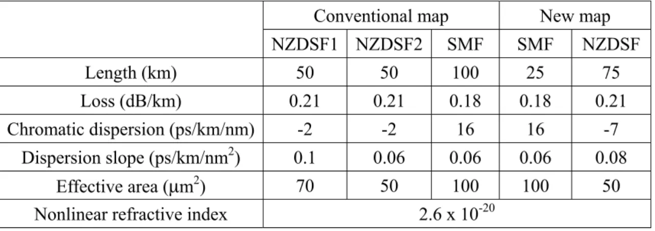
(21) waveform used for the two arms of the Mach-Zehnder modulator was a raised cosine with the NRZ format. The RZ waveform was also the raised cosine and applied after the PSK modulator. Two different dispersion maps were simulated. The first one was the conventional map, and the other one was the new map proposed in reference [4]. Both maps were comprised non-zero dispersion shifted fiber (NZDSF) and conventional single mode fiber (SMF), but the parameters of the fibers were a little different. Table 2.1 shows the summary of the parameters of those fibers. The conventional map included the SMF span and eight NZDSF spans to construct one unit, and the SMF span were installed in the center of the unit. Each NZDSF span comprised NZDSF1 and NZDSF2. The differences of these two fibers were (I) NZDSF1 had larger effective area (II) NZDSF2 had smaller dispersion slope. The new map comprised hybrid spans except for both ends of the transmission line. The hybrid span was composed of the SMF and the NZDSF, while only the SMF were used for both ends. Figure 2.5 shows the cumulative dispersion of these maps at 1550nm. While the conventional map compensated the cumulative dispersion periodically, the new map compensated the cumulative dispersion only at both ends. The averaged zero dispersion wavelength of both maps was set to 1550nm, and the transmission distance were 6300km for the conventional map and 6360km for the new map. The repeater output power was varied between +10dBm and +15dBm with 1dB step. The noise figure of the repeater was set to 4.5dB. The wavelength dependent gain of the repeater was ignored in this simulation. The number of the repeater was 63 for both maps, and the span length of both maps was 100km. Table 2.1 Fiber parameters for the numerical simulation. Conventional map NZDSF1 NZDSF2. New map. SMF. SMF. NZDSF. Length (km). 50. 50. 100. 25. 75. Loss (dB/km). 0.21. 0.21. 0.18. 0.18. 0.21. -2. -2. 16. 16. -7. 0.1. 0.06. 0.06. 0.06. 0.08. 70. 50. 100. 100. 50. Chromatic dispersion (ps/km/nm) 2. Dispersion slope (ps/km/nm ) 2. Effective area (μm ) Nonlinear refractive index. 2.6 x 10. 15. -20.

(22) Cumulative dispersion (ps/nm). 5000 4000 3000 2000 1000 0 -1000 -2000 -3000 -4000 -5000. Conventional map New map. 0. 2000. 4000. 6000. Transmission distance (km) Figure. 2.5 Cumulative dispersion at 1550nm. The cumulative chromatic dispersion for each channel was compensated at the receiving end, and the residual dispersion after dispersion equalization was set to 100ps/nm. The optical demultiplexer had the Gaussian shape with the bandwidth of 0.1nm. For the signal demodulation, difference of the optical phase was directly calculated from the optical field following the method. The difference of the phase was defined as the phase difference between two sampling points separated by one bit period, and it was shown within the range between –π/2 to 3π/2 to obtain an eye-like diagram of the phase. The performance was evaluated by the Q-factor obtained from the rails of 0 phase and π phase. The calculation method of the Q-factor is shown schematically in Figure 2.6. At first, the phase difference separated by one bit period was calculated, and the eye-like diagram in Fig.2.6 was obtained. The time window was used to get the sampling point. The average and the standard deviation for 0 and π were obtained. Finally, the Q-factor was calculated using the equation (2.1.41). μ and σ in equation (2.1.41) are the average and the standard deviation, respectively, and π and 0 stands for the phase. In general, we use the dB scale to express the Q-factor, and the transform equation is equation (2.1.42) μ − μ0 Q= π (2.1.41) Q[dB] = 10*log (Q2) (2.1.42) σπ + σ 0. 16.

(23) Figure. 2.6 Q-factor calculation using the phase difference. 2.2 Comparison of the dispersion maps 2.2.1 Effects of the repeater output power The transmission performance as a function of the repeater output power was evaluated for the conventional map and the new map. Figure 2.7 shows a comparison of two dispersion maps. The obtained averaged Q-factor is shown as a function of the repeater output power. The highest averaged Q-factors for the conventional map and the new map were 12.4dB and 13.5dB, respectively, with +12dBm repeater output power. For the conventional map, the averaged Q-factor was degraded faster than the new map at more than +12dBm repeater output power. This result implies that the new map has better tolerance to the optical fiber nonlinear effect. The difference of the averaged Q-factor between the two maps became more than 1.5dB when the repeater output power was +15dBm. These results showed clear evidences that the transmission performance of the long-haul RZ-DPSK system could be improved by adopting the new map instead of the conventional map.. 17.

(24) Averaged Q-factor (dB). 15. Conventional map New map. 14 13 12 11 10 9. 10. 11. 12. 13. 14. 15. 16. Repeater output power (dBm) Figure. 2.7 Averaged Q-factor of two dispersion maps. Figures 2.8 and 2.9 shows the transmission performance comparison of two dispersion maps without the SPM effect and the XPM effect, respectively. The obtained averaged Q-factor is shown as a function of the repeater output power. In Figure 2.8, the highest averaged Q-factor for the conventional map was 15.1dB at +14dBm repeater output power, while it was 16.5dB at +15dBm repeater output power for the new map. For the conventional map, the transmission performance was degraded at +15dBm repeater output power, but there was no significant degradation for the new map. The difference of the averaged Q-factor between the two map became more than 2dB when the repeater output power was +15dBm. Even though, the performance of both maps were improved compared to figure 2.7. This means that the SPM degrades the transmission performance of both maps significantly. In figure 2.9, the highest averaged Q-factor for the conventional map and the new map were 13.1dB and 13.9dB, respectively, with +13dBm repeater output power. For the conventional map, the averaged Q-factor was degraded faster than the new map at more than +13dBm repeater output power. This result implies that the new map has better tolerance to the optical fiber nonlinear effect. As the XPM is ignored in this figure, this means that the new map is more tolerable to the SPM than the conventional map. On the other hand, compared to figure 2.7, the transmission performances were almost the same. This implies that the XPM is not a major factor of the performance degradation of the system for both the conventional and the new maps.. 18.

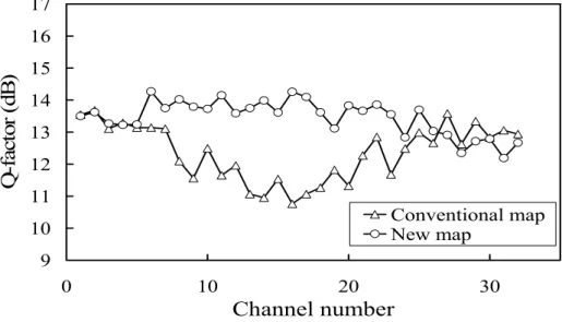
(25) Averaged Q-factor(dB). 17 16 15 14 Conventional map New map. 13 12 9. 10. 11 12 13 14 Repeater Output power (dBm). 15. 16. Figure. 2.8 Averaged Q-factor of two dispersion maps without SPM effect. Averaged Q-factor(dB). 15 14 13 12 Convenntional map New map. 11 10 9. 10. 11 12 13 14 Repeater Output power(dBm). 15. 16. Figure. 2.9 Averaged Q-factor of two dispersion maps without XPM effect. 2.2.2 Individual channel performance In this section, we will discuss the transmission performance at +12dBm repeater output power because it is the highest performance as shown in figure 2.7. Figure 2.10 shows the Q-factors as a function of the channel number for both dispersion maps when the repeater output power was +12dBm. From the figure, we could observe that the performance was almost the same for edge channels, but there was a dip near the center channels for the conventional map, while there was no significant performance degradation near the center channels for the new map. Figure 2.11 shows the eye diagrams of the two dispersion maps in channel 16, because this channel has the highest performance difference as shown in figure 2.10. From these two diagrams we 19.

(26) can observe that the eye of new dispersion map is more clearly opened than the conventional dispersion map. The performance dip near the center wavelength is the same tendency observed in reference [4], and the reason of this phenomenon was attributed to the SPM effect in that reference. Then, the performance without the SPM or the XPM was evaluated. 17. Q-factor (dB). 16 15 14 13 12 11. Conventional map New map. 10 9 0. 10. 20. 30. Channel number Figure. 2.10 Q-factor of two dispersion maps at +12dBm. Eye diagram of new map. Eye diagram of conventional map. Figure 2.11 Eye diagrams of channel 16 at +12dBm repeater output power. Figure 2.12 shows the performance without the SPM, and figure 2.13 shows the performance without the XPM. As shown in figure 2.12, there was no significant dip near the center wavelength for the conventional map, but the performance of the conventional map was still worse than that of the new map. This means that the reason of the performance dip shown in figure 2.10 is mainly due to the SPM, but partially due to the XPM. As the repeater output power is higher than that used in reference [4], it could be considered that the XPM effect became significant enough to contribute the performance degradation near the center wavelength. Still, the XPM 20.

(27) was not the major reason, because the performance dip in the center region was clearly observed in figure 2.13. From these results, it can be concluded that the new dispersion map reduced the nonlinear effect especially the SPM for the long-haul RZ-DPSK transmission, and improved the performance. 17. Q-factor (dB). 16 15 14 13 12 11. Conventional map New map. 10 9 0. 10. 20. 30. Channel number Figure. 2.12 Transmission performance without the SPM effect at +12dBm 17. Q-factor (dB). 16 15 14 13 12 11. Conventional map New map. 10 9 0. 10. 20. 30. Channel number Figure. 2.13 Transmission performance without the XPM effect at +12dBm. Figures 2.14 and 2.15 show the eye diagrams of the channel 16 at +12dBm repeater output power without the SPM and the XPM, respectively. We can observe that when we ignored the SPM effect, the new map showed more clear eye than the conventional map. On the other hand, in the case of without the XPM effect, the eyes were almost the same for both dispersion maps. These results reflect the previously discussed results.. 21.

(28) Eye diagram of new map. Eye diagram of conventional map. Figure 2.14 Eye diagrams of channel 16 without the SPM effect. Eye diagram of new map. Eye diagram of conventional map. Figure 2.15 Eye diagrams of channel 16 without the XPM effect. 2.2.3 Effects of the SPM and the XPM Figures 2.16 and 2.17 show the performance with different conditions of the conventional map and the new map, respectively. As shown in figure 2.16, the performance was largely improved when the SPM effect was ignored especially near the center channel area, while the improvement was small when the XPM effect was ignored. From this result, it can be said that the SPM caused the performance degradation at the center channel of the conventional map. On the other hand, as shown in figure 2.16, even though the performance was improved when the SPM effect was ignored, the improvement was not so significant compared to the conventional map, and the improvement was not channel dependent. The averaged Q-factor without the SPM for the conventional map and the new map were 14.5dB and 15.3dB, respectively. The averaged Q-factor without XPM for the conventional map and the new map were 13.1dB and 13.7dB, respectively. These results show that the SPM caused the wavelength dependent degradation for the conventional map, and there was the significant degradation in the region close to the center wavelength, (i.e., the system zero dispersion wavelength). The XPM played a minor role of the transmission performance degradation of the conventional map while it was virtually no effect for the new map. It can be concluded that the new dispersion map reduced 22.

(29) the effect of both the SPM and the XPM for the long-haul RZ-DPSK transmission and improved the performance. 17 16. Q-factor(dB). 15 14 13 12 11 All effects Without SPM. 10. Without XPM. 9. 1. 5. 9. 13. 17. 21. 25. 29. Channel number. Figure. 2.16 Q-factors of conventional map with different conditions 17 16 15. Q-factor(dB). 14 13 12 11 10 All effects Without SPM Without XPM. 9 8 1. 5. 9. 13. 17. 21. 25. 29. Chennel number. Figure. 2.17 Q-factor of new map with different conditions. 23.

(30) 2.3 Conclusions In this chapter, we used the numerical simulation to evaluate the different repeater output power and different nonlinear effect for the conventional map and the new map. From these simulation results, we observed very clearly that the new map had the better performance than the conventional map especially in high repeater output power region. We also observed the new map had better tolerance to the optical fiber nonlinear effect than the conventional map, especially in the center wavelength region. From these results, it can be concluded that the new dispersion map reduced the nonlinear effect especially the SPM for the long-haul RZ-DPSK transmission, and improved the performance. The SPM played a major role of the transmission performance degradation of the conventional map while there was not so significant effect for the new map. We have conducted the analysis of the transmission performance of the RZ-DPSK system theoretically, and obtained the result that there was a significant influence of the design of the dispersion map. We found that the new map had better performance than the conventional map especially in high repeater output power region. As the major reason of the penalty is the SPM effect of the transmission fiber and it strongly depends on the dispersion map design, it is very important to find a dispersion map that is effective to reduce the nonlinear effect, and the new map in reference [4] is a good example of such a map.. References in this chapter [1] [2] [3] [4]. [5]. [6]. G. P. Agrawal, Fiber-Optic Communication System (Third Ed.), Willy Inter-Science, 2002 J. M. Senior, Optical Fiber Communications Principles and Practice (Second Ed.), 1992 G. P. Agrawal, Nonlinear Fiber Optics (Fourth Ed.), Academic Press, 2006. G. Mohs, W. T. Anderson, E. A and Golovchenko, “A new dispersion map for undersea optical communication systems,” in proc. of Optical Fiber Communication conference (OFC) 2007, paper JThA41, Anaheim, 2007. G. Bosco, A. Carena, V. Curri, R.Gaudino, P. Poggiolini, and S. Beneteddo, “Suppression of spurious tones induced by the split-step method in fiber systems simulation,” IEEE Photon. Technol. Lett., vol.12, no.5, pp.489-491, 2000. X. Wei, X. Liu, and C. Xu, “Numerical simulation of the SPM penalty in a 10-Gb/s RZ-DPSK system,” IEEE Photon. Technol. Lett., vol.15, no.11, pp.1636-1638, 2003. 24.

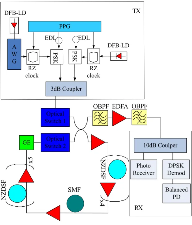
(31) Chapter 3 Experimental study of the nonlinear effects upon long-haul RZ-DPSK system 3.1 Introduction As explained in chapter 2, the nonlinear effects cause the performance degradation of the long-haul RZ-DPSK system. The important features observed through the numerical simulations are (1) the XPM does not cause any significant performance degradation, and (2) the SPM causes a significant degradation near the system zero dispersion wavelength. It is important to confirm these features experimentally. This chapter is devoted to this issue.. 3.2 Experimental Setup In this section, the experimental setup is explained separately by three parts: the transmitter part, the transmission line part, and the receiver part. Figure 3.1 shows the experimental setup schematically.. 25.

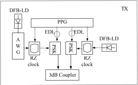
(32) TX. DFB-LD PPG EDL. EDL DFB-LD PSK. PSK. A W G RZ clock. RZ clock 3dB Coupler. OBPF EDFA OBPF Optical Switch 1 Optical Switch 2. 10dB Coulper Photo Receiver. SMF x4. NZDSF. NZDSF. x5. GE. DPSK Demod Balanced PD. RX. Figure 3.1 Experimental Setup. 3.2.1 Transmitter Figure 3.2 shows a configuration of the transmitter schematically. Seven DFB-LDs were used as the light sources, and their wavelengths were ranged from 1547.6nm to 1552.4nm with 0.8nm channel separation. Six DFB-LDs except the center channel multiplexed by an arrayed waveguide grating (AWG) multiplexer. A Mach-Zehnder modulator and a PSK modulator were connected in series after the DFB-LD and the AWG. The Mach-Zehnder modulator was made of a LiNbO3 crystal. The purpose of the Mach-Zehnder modulator was to generate RZ-waveform in the 26.

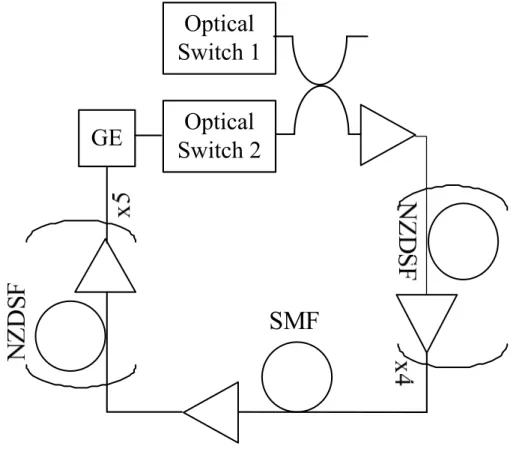
(33) intensity. The clock of the pulse pattern generator (PPG) had a sinusoidal waveform and injected into the Mach-Zehnder modulator to generate the RZ waveform. The PSK modulator was driven by a pseudorandom pattern from the PPG. The electrical delay line (EDL) was connected between the PPG and the PSK modulator in order to synchronize the RZ waveform and the phase modulation. The modulation bit-rate and the patter were 11.4Gbit/s and 215 -1, respectively. The reason why two individual transmitters were used was that the XPM effect should be evaluated experimentally, and this issue is explained in a latter section.. Figure 3.2 Transmitter configuration. 3.2.2 Transmission line Figure 3.3 shows a schematic diagram of the transmission line. There were ten spans of optical fibers and eleven erbium-doped fiber amplifiers (EDFAs). Total length of the transmission line was 495km. The optical fibers used for the experiment were the non-zero dispersion shifted fiber (NZDSF) and the conventional 1.3μm zero dispersion single mode fiber (SMF). The first span to the fourth span and the sixth span to the last span were the NZDSF, and the fifth span was the SMF to form the dispersion map. This kind of a dispersion map is commonly used in the commercial long-haul undersea communication system. Figure 3.4 shows a schematic of the dispersion map. The averaged zero dispersion wavelength of 495km transmission line was 1550nm. The length of each span was 50km for the NZDSF and 45km for the SMF. In the NZDSF span, we used two different effective area fibers. The first 30km was a large effective area fiber and the remaining 20km was a small effective area fiber. The effective area of the large fiber and the small fiber were 70μm2 and 50μm2, respectively. The averaged fiber loss of each span was 11.5dB for the NZDSF and 9dB for the SMF. The parameters of the fiber were shown in Table 3.1. The EDFAs 27.

(34) compensated the loss of the transmission fiber. The gain and noise figure of the EDFAs were 11.5dB and 4.5dB, respectively. The EDFA output power was varied between +2dBm and +8dBm with 1dB step. A gain equalizer (GE) was inserted after the transmission line, and it compensated the wavelength response of the EDFA chain to be flat enough for the WDM transmission.. Optical Switch 1 GE. Optical Switch 2. SMF. chromatic dispersion (ps/nm/km). Figure 3.3 Transmission line configuration. 600 500 400 300 200 100 0 -100 -200 -300. 495km. -400 -500. 0. 100. 200. distance (km). 300. 400. Figure 3.4 Dispersion map of the experiment. 28. 500.

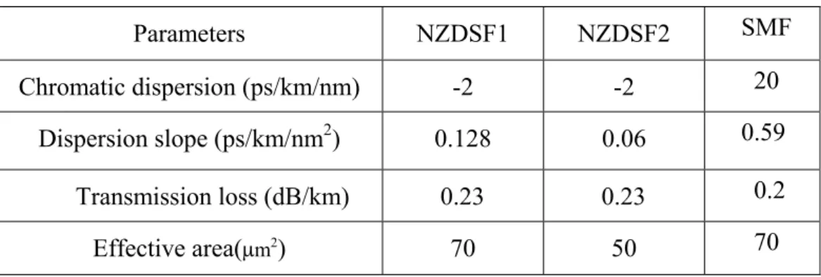
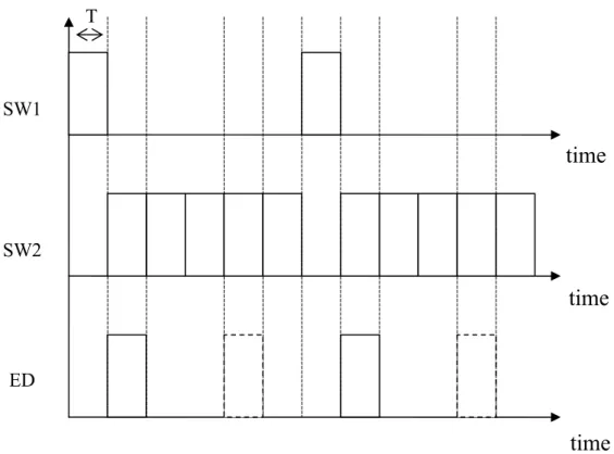
(35) Table 3.1 Parameters of the transmission fiber. Parameters. NZDSF1. NZDSF2. SMF. Chromatic dispersion (ps/km/nm). -2. -2. 20. Dispersion slope (ps/km/nm2). 0.128. 0.06. 0.59. 0.23. 0.23. 0.2. 70. 50. 70. Transmission loss (dB/km) Effective area(μm2). 3.2.3 Operation of recirculating fiber loop. A recirculating fiber loop experiment is an important experimental technique to study a long-haul optical fiber communication system. It enables to realize several thousands kilometer transmission in the laboratory. In order to measure the bit error rate after the long-distance transmission, a control of the timing is important for the recirculating loop experiment. Figure 3.6 shows the timing trigger diagram of the recirculating fiber loop. The duration of each pulse is determined by the round trip time of the transmission fiber. The exact length of the transmission fiber in this experiment was 497.189055km. As the refractive index of the fiber is 1.475 and the light velocity in vacuum is C=2.99792458*108(m/s), the light velocity in the fiber C’ can be calculated as C'=. C n. (3.1.1). where n is the refractive index of the fiber. Then, C’ = 2.032491241*108 (m/s). From these parameters, we can obtain the round trip time T using C’. T=. L = 2.446205155(ms ) C'. (3.1.2). T corresponds to the unit duration of each pulse. L is the length of the transmission line. From the calculation, the duration of each pulse was defined.. 29.

(36) T. SW1. time. SW2. time. ED. time Figure 3.5 Trigger timing of the recirculating loop. As shown in figure 3.5, switch 1 turns on and switch 2 turns off first. The optical signal from the transmitter passes through the 3dB coupler and go into the transmission line and the receiver. The receiver receives the signal directly from the transmitter, and this means that the receiver receives the signal in back-to-back condition. Simultaneously, the signal travels through the transmission line. Then, for the next period, the switch 2 turns on and switch 1 turns off. The signal is allowed to pass through the switch 2 and the 3dB coupler, and go into the transmission line and the receiver again. This process is repeated until required transmission length is achieved. In order to measure the BER using the error detector (ED), the trigger is provided to activate the ED like the third column of figure 3.5. For example, if we want to measure the transmission performance after 2000km, the trigger to the ED turns on at the forth period like a dash line in figure 3.5. Thus, the period of switch 2 determines the maximum transmission distance, and the trigger of the ED chooses what transmission distance to be measured. This is a general explanation of the timing control of the recirculating loop experiment. In the long-haul optical fiber communication system, there is one important factor to affect the performance, the optical signal-to-noise ratio (OSNR). The OSNR means the difference between the optical signal power and the ASE noise. The higher 30.

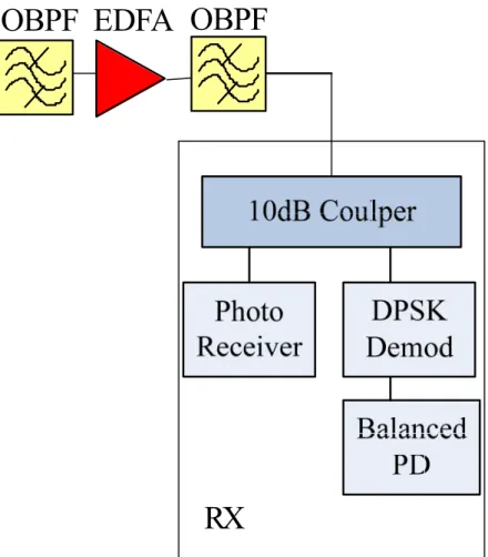
(37) OSNR can achieve the better transmission performance. The OSNR can be calculated by the theoretical equation and can be measured experimentally. In the long-haul transmission experiment, it is important to compare the theoretical OSNR and the experimental OSNR to validate the health of the experimental setup. To calculate the theoretical OSNR, we need to calculate the total ASE power using equation (3.1.3). PASE = 2nsp hν 0 N A (G − 1)Δν opt. (3.1.3). where nsp is the spontaneous-emission factor and it is written as 2nsp=Fn,. Fn is the noise figure of the EDFA. h is the plank constant. ν0 is the frequency of the optical signal. NA is the number of the EDFAs in the transmission line. G is the gain of the EDFA, and Δνopt is the bandwidth of the optical filter. Then, the OSNR can be written as OSNR = Pin / PASE. (3.1.4). When we set the repeater output power to +5dBm, ν 0 to 1550nm, NA to 11, G to 11.5dB, and Δνopt to 0.1nm, the OSNR of the transmission line is calculated to be 22.8dB after 500km transmission. The measured OSNR was 23dB and it was almost the same with the theoretical calculation. After 5000km transmission, the measured OSNR was decreased to 13dB because the number of amplifiers was increased. From these results, it was confirmed that the transmission line had no significant problem.. 3.2.4 Recevier Figure 3.7 shows a schematic of the optical receiver. There were two 0.7nm optical bandpass filters (OBPF) in cascade to select the wavelength to be measured. An EDFA was inserted as a preamplifier to improve the receiver sensitivity. Another OBPF was used to filter out the ASE noise of the preamplifier. The 10dB coupler was used to separate the optical power to the DPSK demodulator and the photo receiver. The photo receiver provided a recovered clock to measure the Bit-error-rate (BER) performance. After the DPSK demodulator, there was a balanced photo receiver and it transformed the optical signal to the electrical signal. The transmission performance was evaluated by the BER, and it was transformed to the Q-factor in dB scale. The transformation equation can be written as 1 Q exp(−Q 2 / 2) BER = erfc( ) ≈ 2 2 Q 2π. (3.1.5). We used the matlab program to calculate the Q-factor from BER. Then, the Q-factor 31.

(38) is changed to the dB scale using equation (3.1.6) Q[dB] = 10 log(Q 2 ). (3.1.6). Using these equations, the transmission performance is described by the Q-factor in dB scale.. Figure 3.6 Schematic of the optical receiver. 3.3 Measurement of the transmission performance In this section, the experimental result after 5000km transmission is presented and discussed. In section 3.3.1, the transmission performance as a function of different repeater output power from +2dBm to +8dBm is discussed. Section 3.3.2 describes the transmission performance of different signal wavelength. Section 3.3.3 is the experimental investigation of the effect of the XPM. Section 3.3.4 is the experimental investigation of the effect of the SPM.. 32.

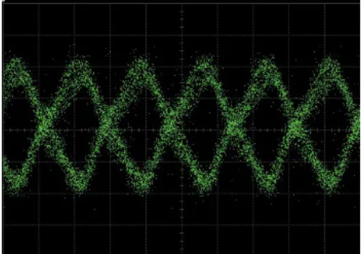
(39) 3.3.1 Performance dependence upon the repeater output power The first step of the experiment is the performance of different repeater output power after 5000km transmission. The repeater output power was varied from +2dBm to +8dBm with 1dB step. The signal wavelength was 1550nm. Figures 3.7 to 3.13 show the eye diagram for the different repeater output power. All these eye diagrams were measured with 100mv/div vertical scale and 50.0ps/div horizontal scale.. (a) after 500km transmission. (b) after 5000km transmission. Figure 3.7 +2dBm repeater output power. (a) after 500km transmission. (b) after 5000km transmission. Figure 3.8 +3dBm repeater output power. (a) after 500km transmission. (b) after 5000km transmission. Figure 3.9 +4dBm repeater output power. 33.

(40) (a) after 500km transmission. (b) after 5000km transmission. Figure 3.10 +5dBm repeater output power. (a) after 500km transmission. (b) after 5000km transmission. Figure 3.11 +6dBm repeater output power. (a) after 500km transmission. (b) after 5000km transmission. Figure 3.12 +7dBm repeater output power. 34.

(41) (a) after 500km transmission. (b) after 5000km transmission. Figure 3.13 +8dBm repeater output power. Figure 3.14 shows the transmission performance of different repeater output power after 5000km transmission. It shows the obtained Q-factor as a function of the repeater output power. From this figure, the best and the worst Q-factor were 8.0dB and 7.8dB for +5dBm and +8dBm repeater output power, respectively.. 8.1 8.05 Q-factor(dB). 8 7.95 7.9 7.85 7.8 7.75 7.7 0. 1. 2. 3. 4. 5. 6. 7. 8. 9. Repeater Output Power (dBm). Figure 3.14 Q-factor of different repeater output power after 5000km transmission. The reason of the worst transmission performance at +8dBm can be attributed to the increased nonlinear effect due to the higher repeater output power. The tendency of this experimental result is similar as the simulation result, and the suitability of the simulation was confirmed through the experiment.. 35.

(42) 3.3.2 Performance of different wavelength after 5000km transmission. Q-factor(dB). The theoretical study discussed in chapter 2 showed that the transmission performance was degraded close to the system zero dispersion wavelength. Therefore, wavelength dependence of the transmission performance was measured. The measured wavelengths were 1548.4nm, 1550nm, and 1551.6nm. They were selected because there were enough dispersion compensation fiber to cancel the accumulated dispersion after 5000km transmission. For 1548.4nm and 1551.6nm wavelengths, the accumulated chromatic dispersion were -680ps/nm and +750ps/nm, respectively. The dispersion compensation fibers used in this experiment were +685ps/nm and – 750ps/nm, respectively. The repeater output power of this experiment was set to +4dBm because it had almost the best performance as +5dBm repeater output power. The experimental result is shown in figure 3.15. The best and the worst Q-factors were 8.6dB and 8.0dB for 1551.6nm and 1550nm, respectively. It was clearly observed that the transmission performance of the center wavelength degraded larger than the other wavelengths. This result also matched with the tendency of the simulation result in chapter 2.. 8.7 8.6 8.5 8.4 8.3 8.2 8.1 8 7.9 1548. 1549. 1550 1551 Wavelength(nm). 1552. Figure 3.15 Measured Q-factor for different wavelengths. 3.3.3 Experimental investigation of the effect of the XPM In the simulation result discussed in chapter 2, the difference of the transmission performance with and without the XPM effect was not so significant. Then, it was confirmed by an experiment. Figure 3.16 shows a simple explanation how to eliminate the XPM effect in the experiment. The XPM effect is caused by the neighboring wavelengths that are modulated. To eliminate the XPM effect, the 36.

(43) simplest way is to turn off the modulation of the neighboring channels, but it is required to keep the same optical power to maintain other nonlinear effects as the same. Therefore, it is required to have a modulated signal channel and continuous wave (CW) neighboring channels. Figure 3.17 shows the optical spectrum before the transmission. It is quite clear that just only the center channel was modulated but the others were not.. (a) All channels modulated. CW. CW. Modulated CW. CW. (b) Only modulated measured channel Figure 3.16 Method to eliminate the XPM effect. Figure 3.17 Optical spectrum before transmission. 37.

(44) Q-factor(dB). The repeater output power were set to +4dBm and +5dBm, because these two repeater output power had almost the best transmission performance in section 3.3.1. Figure 3.18 and 3.19 shows the transmission performance for two different repeater output powers. The transmission distance was varied from 3000km to 5000km. Before 3000km transmission, the BER was error free. The performance without the XPM effect after 5000km transmission for +4dBm and +5dBm repeater output power were 8.0dB and 8.1dB, respectively. The performance difference after 5000km transmission between with and without XPM were 0.6dB and 0.1dB for +4dBm and +5dBm repeater output power, respectively. From these figures, it can be observed that the performance without the XPM effect is better than that with the XPM effect, but the difference is not so significant. This result means that the XPM effect was not a major reason of the degradation factor of this transmission system. It can be said that the simulation result was confirmed through the experiment.. 17 16 15 14 13 12 11 10 9 8 7 6 2500. With XPM effect Without XPM effect. 3000. 3500. 4000. 4500. 5000. 5500. distance(km) Figure 3.18 Measured Q-factor of +4dBm repeater output power as a function of transmission distance. 38.

(45) 17 16. Q-factor(dB). 15 14 13 12 11 10 9 8. With XPM effect Without XPM effect. 7. 2500. 3000. 3500. 4000. 4500. 5000. 5500. distance(km) Figure 3.29 Measured Q-factor of +5dBm repeater output power as a function of transmission distance. 3.3.4 Experimental investigation of the effect of the SPM In the previous section, the XPM effect is confirmed through the experiment. In this section, the SPM effect is evaluated by experiment. It is very difficult to eliminate the SPM effect in the actual experiment because the SPM is caused by the signal intensity itself. To investigate the effect of the SPM upon the transmission performance, following experimental configuration was used. The repeater output power was set to +8dBm, but the power of the selected channel to be measured was reduced by 1dB step compared to the other channels. If the channel power is reduced by 1dB, the measurement channel has 1dB smaller signal power, and this signal power corresponds to the power of +7dBm repeater output power. Figure 3.20 shows a simple explanation of this configuration. The measured channel power was reduced by 0dB to 6dB with 1dB step, and it corresponded to +8dBm to +2dBm repeater output power. In this condition, we can confirm the SPM effect because the signal power was reduced and the SPM effect also reduced. Figure 3.21 shows the measured OSNR for different repeater output power. The dash line was the original experimental results, it means the power of every channel was the same and used the different repeater output power from +2dBm to +8dBm. The direct line was using fixed +8dBm repeater output power but the measurement channel power was reduced by 1dB step to realize the same signal power as the different repeater output power, and the other channel powers were maintained to the 39.

(46) original power. From this figure, it can be observed that the OSNR of the measured channel was improved for the fixed repeater output power case shown by the direct line. This is because the repeater output power was increased to +8dBm and other WDM channels had the corresponding power. Figure 3.22 shows the performance after 5000km transmission. The direct line shows the performance of the fixed repeater output power, and the dash line shows the performance of the variable repeater output power. From this figure, it can be observed that the performance of the fixed repeater output power case was improved significantly when the signal power was suppressed by a few dB. The best performance was occurred when the signal power was decreased by 4dB. This condition corresponded to +4dBm repeater output power. The OSNR at +5dBm repeater output power was better than that of this case, but the Q-factor of this case was significantly better than that of +5dBm repeater output power with flat WDM signal power case. This result implied that the reduction of the SPM could improve the transmission performance significantly. It can be said that the simulation result have been confirmed by the experimental result.. Other channels. 1dB reduced. Measurement channel. Figure 3.20 Explanation of the SPM effect experimental setup. 40.

(47) 17 16. OSN R (dB). 15 14 13 12. Fixed +8dBm repeater output power With same channel power. 11 10 9 8 0. 1. 2. 3. 4. 5. 6. 7. 8. 9. Corresponding repeater output power (dBm) Figure 3.21 Measured OSNR after 5000km transmission 11.5. With same channel power. 11. Fixed +8dBm repeater output power. Q-factor (dB). 10.5 10 9.5 9 8.5 8 7.5 7 1. 2. 3. 4. 5. 6. 7. 8. 9. Correspond repeater output power (dBm). Figure 3.23 Measured Q-factor after 5000km transmission. 41.

(48) 3.3.5 Discussion This experiment used the conventional map of the simulation in chapter 2. From these experimental results, there were a few important observations. First, the optimum repeater output power was around +5dBm. Second, the performance was degraded near the system zero dispersion wavelength, but it was improved when the wavelength was shifted from that wavelength. Third, the XPM effect did not cause so significant performance degradation in the transmission. Forth, it looked like that the SPM effect caused significant performance degradation in the transmission. In the experiment, 5000km transmission was achieved using the conventional map with the RZ-DPSK format. Through the experiment, the simulation results of chapter 2 was qualitatively confirmed.. 3.4 Conclusion Experimental study of the transmission performance of the long-haul RZ-DPSK system was conducted using the recirculating loop setup. The obtained results were basically reasonable compared to the theoretical simulation results in chapter 2. Therefore, it can be concluded that the nonlinear effects are important factors for the long-haul RZ-DPSK system.. 42.

(49) Chapter 4 Conclusion In this master thesis, the difference of the transmission performance of the long-haul RZ-DPSK system due to the different dispersion map and repeater output power was studied through the numerical simulation and experiment. In the simulation, the numerical simulator which was designed to isolate the nonlinear effects was used to evaluate the transmission performance of the long-haul RZ-DPSK system. The simulation was done to use conventional dispersion map and new dispersion map for the different repeater out put power. First, the effect of different repeater output power for the conventional map and the new map was investigated. The repeater output power was varied between +10dBm and +15dBm with 1dB step. The best averaged Q-factor for the conventional map and the new map was occurred with +12dBm repeater output power. For the conventional map, the Q-factor was degraded faster than the new map at more than +12dBm repeater output power. This result implies that the new map has better tolerance to the optical fiber nonlinear effect and also shows the clearly evidence that the transmission performance of the long-haul RZ-DPSK system could be improved by adopting the new map instead of the conventional map. Second, transmission performance of +12dBm repeater output power was investigated for both dispersion maps because it was the best repeater output power. From the result, it was observed that the SPM was the major reason of the performance degradation and the XPM was not. For the conventional map, the performance dip was observed near the center wavelength but there was no significant performance degradation in the edge region. For the new map, there was no significant performance degradation near the center wavelength. To confirm the theoretical simulation, the experiment was conducted. The repeater output power was varied from +2dBm to +8dBm with 1dB step. The best Q-factor was 8.0dB at +5dBm repeater output power. The simulation result using the conventional map was confirmed through the experiment. The result showed that the performance had the same tendency with the simulation. The Q-factor of near the edge wavelength was better than the center wavelength. For the optical fiber nonlinear effect, the XPM and the SPM effects were investigated. The Q-factor without XPM effect was a little better than that with the XPM effect but almost the same. For the SPM effect, the performance with reduced SPM was improved significantly than that with the SPM. From these experimental results, it can be concluded that the SPM is the most important factor in the conventional map.. 43.

(50) In this master thesis, followings were achieved.. [1] The transmission performance of the long-haul RZ-DPSK system with the conventional dispersion map and the new dispersion map was evaluated through the numerical simulation. [2] The new map was confirmed to have better transmission performance than the conventional map especially in higher repeater output power region. [3] The major reason of the performance penalty of the long-haul RZ-DPSK system was the SPM effect and the minor reason was the XPM effect. [4] The coincidence of the theory and the experiment was confirmed.. As these achievements are significant enough to contribute the progress of the optical fiber communication system, this master thesis was successful.. 44.

(51) List of Abbreviations. RZ-DPSK SPM XPM PSK CW NLS PRBS BER NRZ NZDSF SMF WDM AWG PPG EDL EDFAs GE ED OSNR ASE OBPF PD MUX DEMUX DFB-LDs TX RX. Return to Zero Differential Phase Shift Keying Self-Phase Modulation Cross-Phase Modulation Phase Shift Keying Continuous Wave NonLinear Schrödinger Pseudo Random Bits Sequence Bit Error Rate Non-Return to Zero Non-zero Dispersion Shifted Fiber Single Mode Fiber Wavelength Division Multiplexing Arrayed Waveguide Grating Pulse Pattern Generator Electrical Delay Line Erbium-Doped Fiber Amplifiers Gain Equalizer Error Detector Optical Signal to Noise Ratio Amplifier Spontaneous Emission Optical BanPass Filter Photo Detector Multiplexing Demultiolexing Distributed FeedBack Laser Diodes Transmitter Receiver. 45.

(52)