國
立
交
通
大
學
資訊工程學系
資訊科學與工程研究所
碩
士
論
文
針對畫質與
頻寬限制的
串流系統,使用自適
性跳畫面機制的初步探討
A Preliminary Study on
Adaptive Frame Skipping for Quality-and
Rate-Constrained Streaming Systems
研 究 生:林岳進
指導教授:彭文孝 博士
針對畫質與頻寬限制的串流系統,使用自適性跳畫面機制的
初步探討
A Preliminary Study on
Adaptive Frame Skipping for Quality-and
Rate-Constrained Streaming Systems
研究生 : 林岳進
Student: Yuei-Chin Lin
指導教授: 彭文孝 博士
Advisor:
Dr. Wen-Hsiao Peng
國 立 交 通 大 學
資 訊 工 程 學 系
資 訊 科 學 與 工 程 研 究 所 碩 士 班
碩 士 論 文
A Thesis
Submitted to Department of Computer Science College of Electrical and Computer Engineering
National Chiao Tung University in Partial Fulfillment of the Requirements
for the Degree of Master in
Computer Science
September 2008
Hsinchu, Taiwan, Republic of China
針對畫質與頻寬限制的串流系統,使用自適性跳
畫面機制的初步探討
研究生: 林岳進
指導教授: 彭文孝 博士
國立交通大學
資訊工程學系 資訊科學與工程研究所碩士班
摘要
由於人眼對於畫質好壞差異的感受比斷斷續續畫面所帶來的停頓效果較不 敏感,大多編碼器都會注重在將可用位元數分配到所有可編畫面上,即使個別畫 面會因此得到較少的可用位元而使得畫質變差,也大多不願意將畫面率降低來得 到較好的畫質。但是對於監控系統或是一些比較在意畫面品質的攜帶型設備而 言,則會對於編碼畫面品質上有一定要求。 因此如何在同時具有畫質與頻寬限制的環境達到最佳化變成我們想要解決 的議題。為了解決多重限制的問題,我們首先從了解最佳解的設計出發,再深入 研 究 如 何 輔 以 Lagrange multiplier 的 方 式 來 達 到 位 元 率 - 失 真 交 換 下 (Rate-Distortion Trade-Off)最佳化。 相較於一般流量控制的設計都是只考量頻寬限制的要求,我們的問題勢必 要 使 用 動 態 規 劃 才 能 達 到 最 佳 位 元 分 配 ; 然 而 為 了 降 低 複 雜 度 , 支 配 線 (Dominative Line)與依次精修(Successive Refinement)的方法被提出並且分析A Preliminary Study on Adaptive Frame Skipping for Quality-and
Rate-Constrained Streaming Systems
Student: Yuei-Chin Lin
Advisor: Dr.
Wen-Hsiao Peng
Department of Computer Science &
Institute of Computer Science and Engineering
National Chiao Tung University
Abstract
Owing to that human eyes are more sensitive to jerky effect caused by different frame rate rather than quality variance caused by different quality of coded frames, most encoder systems focus on distributing available bit budget among all frames and are not willing to reduce frame rate to obtain better spatial resolution, even the quality of each frame becomes worse for getting less available bits. However, there exists quality requirements to surveillance systems and some mobile devices which care about the quality of each coded frame.
As a result, how to solve the problem with both distortion- and rate-constraint is the main issue in our research. In order to solve this multiple constrained problem, we start by understanding the design of optimal solution; furthermore, we study how to use Lagrangian parameters for rate-distortion trade-off optimization.
Compared with general rate control scheme, which only consider the rate/budget requirement, our problem must use dynamic programming for optimal bit allocation. Nevertheless, in order to reduce complexity, dominative line and successive
誌謝
在這兩年的研究生涯中,我首先要感謝指導教授彭文孝老師。從碩一開始 進實驗室到碩二畢業的兩年間,老師不僅在研究上給予我專業的指導,也同時教 導我研究學問的方法與態度。在此僅向老師至上最高的感謝之意。 這篇論文可以完成,也要感謝交大這個大環境,能夠讓我在這塊領域中討 論,並且解決我的疑問。MAPL 就像個大家庭,實驗室提共了豐富的資源與專業 的設備,還有良好的研究環境,讓我能夠在這裡順利的完成學業。我也很感謝實 驗室的雪婷與敏正、志展同學還有渏紋、鴻志、志鴻學長們,可以共同討論,共 同成長。 最後,我也要感謝我的父母林豐熒先生及陳淑女女士與親戚給予的幫助; 另外秋盛、育青、孝嶸等摯友們,在我研究艱困的時候給予精神上的支持。在此 僅將論文獻給所有幫助過我,陪伴我走過求學生涯的所有師長,朋友、同學和家 人。 林岳進 2008 年九月于新竹A Preliminary Study on Adaptive Frame Skipping
for Quality-and Rate-Constrained Streaming
Systems
Advisor: Prof. Wen-Hsiao Peng
Student: Yuei-Chin Lin
Institute of Multimedia Engineering
National Chiao-Tung Univeristy
1001 Ta-Hsueh Rd., 30010 HsinChu, Taiwan
August 2008
Contents
Contents i
List of Tables iii
List of Figures iv
1 Research Overview 1
1.1 Introduction . . . 1
1.1.1 Architecture . . . 1
1.1.2 Objective and Formulation . . . 2
1.2 Related Works . . . 3
1.3 Contribution and Organization of Thesis . . . 5
2 Constrained Optimization Problems : Principles and Applications 6 2.1 Background . . . 6
2.2 Integer Programming . . . 7
2.3 Lagrangian Optimization . . . 8
2.3.1 Optimization Problems with Multilple Constraints . . . 9
2.3.2 Optimization Problems with Single Constraint . . . 12
CONTENTS
3 Related Works 18
3.1 KKT Conditions . . . 18
3.2 Viterbi Algorithm with Lagrangian Cost . . . 20
3.3 Variable Frame Rates Encoding . . . 21
3.4 Comparison . . . 23
4 Experiments and Analyses 25 4.1 Optimal Solution Analyses . . . 25
4.1.1 MSE Weighting E¤ect . . . 26
4.1.2 Optimal Path Analyses . . . 29
4.2 Proposed Heuristic Solution . . . 32
4.2.1 Coding Frame Selection Methodologies . . . 32
4.2.2 Successive Re…nement . . . 34
4.3 Proposed Rate Control Mechanism . . . 36 5 Conclusions and Future Works 39
List of Tables
2.1 Complexity comparison between DP . . . 17 3.1 Comparison among the proposed problem and related works . . . 23
List of Figures
1.1 Proposed video streaming system architecture. . . 2 1.2 Proposed adaptive frame coding. . . 3 2.1 Illustration of dynamic programming, integer programming and Viterbi
algorithm. . . 7 2.2 Methodologies for constrained optimization problem. . . 7 2.3 Illustration of integer programming. . . 8 2.4 For each independent source, moving the violated value to boundary
value achieves minimal Lagrangian cost based on independent and con-vex properties. . . 11 2.5 Illustration of water …lling principle. . . 12 2.6 Illustration of optimization solution by minimal Lagrangian cost. . . 13 2.7 Di¤erent quantizer choice for frame 1 leads to di¤erent R-D curve of
frame 2, also the solution of minimal lagrangian cost to dependent problem. 14 2.8 Illustration of Viterbi algorithm with minimal Lagrangian cost path in
IBBP case. . . 15 2.9 VA with skip nodes . . . 16 3.1 Illustrative example of the Viterbi algorithm with skip nodes. . . 21
LIST OF FIGURES 4.1 Our experiment procedures. . . 26 4.2 Total MSE(a), coded frames MSE(b) and copy frames MSE(c) in Akiyo
when encoding 2 frames. . . 27 4.3 Total MSE(a), coded frames MSE(b) and copy frames MSE(c) in Mobile
when encoding 2 frames. . . 28 4.4 Total MSE in Akiyo(a) and in Mobile(b) when encoding 7 frames. . . . 28 4.5 Optimal path from low bit budget to high bit budget of (a)Akiyo,
(b)Mobile, (c)Football. . . 29 4.6 Overall distortion may interlace in static sequence like Akiyo(a); the
correct Qp selection for each coding frame may not only reduce coding bits but also reduce overall distortion(b); while available bit budget de-creases, the optimal solution may choose di¤erent frames to be encoded instead of skipping another frame immediately(c). . . 30 4.7 Dominative lines of di¤erent total number of coded frames. . . 31 4.8 Illustration of heuristic solution for independent problem with multiple
constraints by Viterbi algorithm. . . 32 4.9 Illustration of methodology 1. . . 33 4.10 Illustration of methodology 2. . . 33 4.11 Comparison among proposed heuristic solution, methodology 1 and
method-ology 2 in Akiyo (a), Mobile(b) and Football(c). . . 34 4.12 Illustration of successive re…nement. . . 34 4.13 Comparison among proposed heuristic solution and its successive
re…ne-ment(a), methodology 1 and its successive re…nement(b), methodology 2 and its successive re…nement(c) in Akiyo. . . 35 4.14 Comparison among proposed heuristic solution and its successive
re…ne-ment(a), methodology 1 and its successive re…nement(b), methodology 2 and its successive re…nement(c) in Mobile. . . 36 4.15 Comparison among proposed heuristic solution and its successive
re…ne-ment(a), methodology 1 and its successive re…nement(b), methodology 2 and its successive re…nement(c) in Football. . . 37 4.16 Proposed algorithm ‡owchart. At the …rst stage to decide which frames
CHAPTER 1
Research Overview
In the beginning of this thesis, we will introduce the blueprint of the proposed quality-and rate-constrained streaming system, including the architecture, the objective quality-and the formulation to our constrained problem; then related works are mentioned. Finally, the contribution and the organization of this thesis are described in the last section.
1.1
Introduction
1.1.1
Architecture
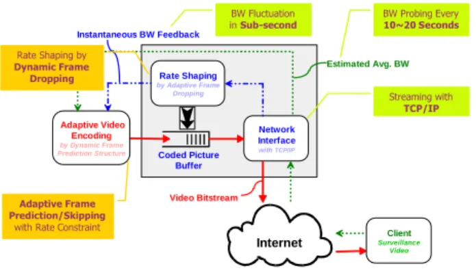
In this section, we propose a quality- and rate-constrained adaptive frame encoding for speci…c video streaming applications such as surveillance and mobile systems. Assume there exists a system architecture like Figure 1.1, the client requires high quality sur-veillance video streaming from the server through the internet TCP/IP transmission. The server has a bandwidth estimation mechanism, which estimates average bandwidth BR in every time slot (10~20 second for example) and we can allocate bits among ref-erence and non-refref-erence pictures according to the estimated BR. However, because network congestion occurs from time to time, we need to provide another rate shaping
Chapter 1. Research Overview Internet Network Interface withTCP/IP Rate Shaping by Adaptive Frame Dropping Coded Picture Buffer Client Surveillance Video Adaptive Video Encoding by Dynamic Frame Prediction Structure Video Bitstream Estimated Avg. BW Instantaneous BW Feedback Streaming with TCP/IP BW Fluctuation
in Sub-second BW Probing Every10~20 Seconds Rate Shaping by
Dynamic Frame Dropping
Adaptive Frame Prediction/Skipping
with Rate Constraint
Figure 1.1: Proposed video streaming system architecture.
mechanism such that coded picture bu¤er can adaptively drop non-reference pictures to adviod short-term bandwidth ‡uctuation.
Within this architecture, we have constraints and requirements as follows: Constraints
–Real-time and live streaming over interenet –Rate- and quality-constrained applications –Time-shifted average bandwidth estimation –TCP/IP connection
Requirements
–A rate- and quality-constrained video encoding scheme –A rate shaping mechanism
1.1.2
Objective and Formulation
In order to implement the above system, we need to provide an adaptive frame encoding that
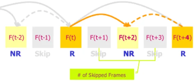
1. Ensures the quality of the reference frames subject to a bitrate constraint. 2. Allows a R-D optimal rate shaping by skipping the non-reference frames.
That is, we have to determine the frames to be skipped from coding and to …nd the quantization parameters for the frames to be encoded,as Figure 1.2, with the following constraints:
1. The bit of total coded frames is equal to bitrate Rt.
Chapter 1. Research Overview F(t+2) F(t+4) F(t) R F(t-1) F(t-2) Skip NR F(t+1) F(t+3) F(t+4) R # of Skipped Frames F(t+1) F(t+3) Skip Skip F(t+1) F(t+3) F(t+1) F(t+3) Skip NR Skip F(t+2) NR F(t+2)
Figure 1.2: Proposed adaptive frame coding.
3. The overall distortion is minimized.
We can further formulate our objectives and constraints as a quality- and rate-constrained optimization problem that
q = arg min q N X i=1 Di(q) s:t: 8 > < > : (1) P i2C Ri(q) Rt
(2i) Dmin Di(q) Dmax;8i 2 C
| {z }
where
Di :Distortion of the ith frame
Ri :Rate of the ith frame
q= [q1; q2; :::; qN]T; qi =f0; 1; :::; 51; 52 Skip
g; i = f1; 2; :::; Ng; C = fi : qi 6= 52; i = f1; 2; :::; Ngg
Owing to only coded frames having distortion constraints, the number of our con-straints is a variable number as (1 + jCj ).
1.2
Related Works
Reed et al: used integer programming to analyze the temporal-, spatial- and psnr-domain optimal bit allocation problem under maximal bu¤er size constraint in [8].
Chapter 1. Research Overview Ortega et al: used integer programming as optimal solution to solve the bu¤er con-strained problem for each individual macroblock in [6], also they applied Lagrange multiplier to a nearly optimal solution for the budget constrained problem. Owing to inter programming tests all possible data set to …nd the optimal solution to multiple constrained or multiple dimensional optimization problems, the solution can be viewed as an absolute optimal solution compared to other algorithms; however, the complexity of integer programming is too large to implement in real time applications. As a result, Lagrangian optimization is applied under several speci…c assumptions in video coding domain for some fast algorithms.
As for optimization problems with multiple constraints by Lagrangian optimiza-tion method, in [5], A. Ortega used Lagrangian method to solve the multiple bu¤er constrained problem by iteratively adjusting Lagrange multiplier . Ahmad et al: ap-plied KKT conditions based on Nash bargaining solution and just-noticeable distortion threshold for each macroblock to solving the perceptual quality constrained problem in [1]. In [12], Wang et al: also applied KKT conditions to each I frames for the long-term distortion constrained problem. Based on KKT conditions, each constraint corresponds to a Lagrange multiplier and the optimal solution occurs when all costraints are sat-is…ed and the Lagrangian cost is at an minimum value by iteratively adjusting each Lagrange multiplier in video domain.
Furthermore, Ramchandran et al: made use of Viterbi algorithm with Lagrangian cost to solve the dependent constrained problem and developed pruning rules based on monotonicity property for the optimization problem with single constraint in [7]. Then Liu et al: improved this pruning algorithm for frame skipping situation in [4]. In order to implement adaptive frame skipping in real time system, Song et al: pre-de…ned Lagrange multiplier and which frames to be encoded for each sub-GOPs, and solved the problem by grandient search in [11]. Because we only have to adjust one Lagrangian multiplier to the optimize problem with single constraint, Viterbi algorithm is applied based on dependent relation and monotonic property. Also, a fast algorithm is developed based on independent relation and commonly used in modern encoder structure.
All constrained problems can be solved by dynamic programming either in con-strained form or unconcon-strained form (Lagrangian method), though the complexity is
Chapter 1. Research Overview huge. In order to reduce complexity, modern rate constrained bit allocation prob-lem develop Lagrangian cost algorithm based on independent property for real time applications.
1.3
Contribution and Organization of Thesis
Specially, our main contributions in this work include the following: Model for Quality- and Rate-constrained Adaptive Frame Encoding
We de…ne our adaptive frame encoding problem as a optimization problem and with multiple constraints and survey kinds of methodologies to solve constrained problems.
Design of Search Strategies for Optimal Solutions
We implement the dynamic programming to obtain the optimal solution to our quality- and rate- constrained problem and …nd out the optimal path is a stairway-like curve; besides, we compare the complexity of di¤erent dynamic programming algorithms.
Propose a Heuristic Algorithm Based on Successive Re…nement
We propose a greedy heuristic algorithm based on independency assumption and successive re…nement to reduce complexity after observing the optimal solution. The remaining of this thesis is organized as follows: Chapter 2 contains a survey of constrained optimization problem, and the di¤erences between our problem and other previous works are also compared. Chapter 4 presents the optimal solution and its analysis in the beginning and then we introduce our heuristic solution and the experimental results; also, an iterative algorithm with lower complexity is proposed in the end. This thesis ends with the summary of our observations and a list of future works.
CHAPTER 2
Constrained Optimization Problems :
Principles and Applications
We will introduce the theory background such as integer programming, Lagrangian optimization and Viterbi algorithm for optimizing constrained problems in detail in the chapter.
2.1
Background
In this section, we will introduce the methodologies to optimize constrained problems and the dynamic programming is commonly used like integer programming and Viterbi algorithm.
A simple algorithm for constrained optimization problem is to …nd the optimal solu-tion among possible data set by dynamic programming and this algorithm is developed as integer programming; on the other hand, the Lagrange multiplier is another math-ematical tool to optimize constrained problems, and the Viterbi algorithm as forward dynamic programming is applied. Although integer programming and Viterbi algo-rithm are all trellis-based algoalgo-rithm, the number of nodes at each stage is constant in
Chapter 2. Constrained Optimization Problems : Principles and Applications VA Inte ge r Programming Dynamic Programming
Figure 2.1: Illustration of dynamic programming, integer programming and Viterbi algorithm.
Dependent Independent
Dependent Independent
Generalized Lagrangian Optimization Unconstrained Optimization Constrained Optimization
Constrained Optimization Problem
Integer Programming Lagrange Multiplier
Single (Equality) Constraint Multiple (Equality+Inequalities) Constraints
KKT Conditions
Constant Slope Viterbi Algorithm Water Filling Principle Integer Programming
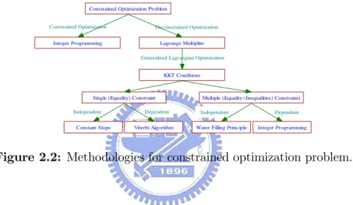
Figure 2.2: Methodologies for constrained optimization problem.
Viterbi algorithm but is variable in integer programming. The relation among dynamic programming, integer programming and Viterbi algorithm is illustrated in Figure 2.1. Also, Figure 2.2 shows di¤erent methodologies to optimize constrained problems, and we will introduce these methodologies in the following subsections: integer pro-gramming in section 2.2, Lagrangian optimization in section 2.3, water …lling principle in section 2.3.1, and Viterbi algorithm in section 2.3.2.
2.2
Integer Programming
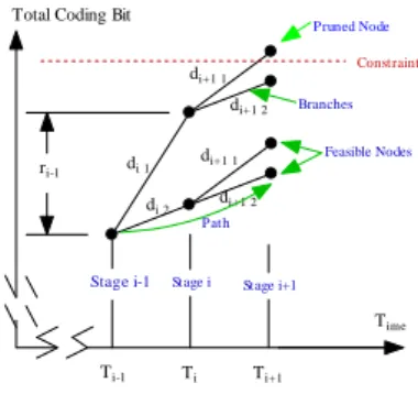
Integer programming is a trellis-based dynamic programming algorithm to solve the constrained problems. Integer programming grows its paths stage by stage and prunes the violated branches to form a trellis from the initial stage to the end stage; as Figure 2.3, the optimal path can be obtained by …nding the node with minimal distortion value at the …nal stage.
Chapter 2. Constrained Optimization Problems : Principles and Applications
Total Coding Bit
Branches Time di+1 2 di+1 2 di 2 di 1 di+1 1 Ti-1 Ti Stage i-1 ri-1 Ti+1 Stage i di+1 1 Stage i+1 Path Feasible Nodes Constraint Pruned Node
Figure 2.3: Illustration of integer programming.
Although the complexity raising exponentially while the number of stage increases, it can be reduced by clustering the operation points to decrease the number of node or using limited-lookahead window optimization to obtain an sub-optimal path at each window size interval [8].
Ortega et al: used the algorithm to solve the problem with bu¤er constraint on each frame [6]. Additionally, Reed et al: analyzed the best solution amaong the combination of spatial, temporal, and psnr dimensions by this algorithm [8].
2.3
Lagrangian Optimization
While dealing with mathematical optimization problems, the method of using Lagrange multiplier can be applied to …nding the extrema of a function of several variables subject to one or more constraints. That is, suppose a function to be minimized, f (x; y), and the solution set is constrained by another function, g(x; y) = 0, the auxiliary function is
J (x; y; ) = f (x; y) + g(x; y) and the minimum occurs when
rx;y; J (x; y; ) = 0
Furthermore, owing to the convexity characteristic of the rate-distortion curve in video coding domain, for a given , the minimum occurs only at the minimal value of J (x; y; ) = f (x; y) + g(x; y). As for optmization problems with multiple
con-Chapter 2. Constrained Optimization Problems : Principles and Applications straints, the generalized Lagrangian optimization, Karush-Kuhn-Tucker conditions, is commonly used; besides, the water …lling principle as a special case of Lagrangian optimization based on independent and convex property is described.
2.3.1
Optimization Problems with Multilple Constraints
2.3.1.1 Karush–Kuhn–Tucker Conditions
The method of using Lagrange multiplier to solve the nonlinear constrained problem is the basic tool in mathematical optimization problems; hence we introduce the gen-eralized Lagrangian optimization (Karush–Kuhn–Tucker Conditions) [3].
Generally, given a optimization problem in the standard form,
min f (x) s:t: 8 < : gi(x) 0; for i = 1; 2; :::; m hj(x) = 0; for j = 1; 2; :::; l
where the objective function f (x) is the function to be minimized, and gi(x), hi(x)
are constraint functions. If x is a local minimum, then there exists constants ui(i =
1; 2; :::; m)and vj(j = 1; 2; :::; n)such that
J (x; u; v) = f (x) + m X i=1 igi(x) + n X j=1 vjhj(x) (1) rxf (x ) + m P i=1 ir xgi(x ) + n P j=1 vjrxhj(x ) = 0 (2) hj(x ) = 0; for j = 1; 2; :::; n (3) gi(x ) 0; for i = 1; 2; :::; m (4) i 0;for i = 1; 2; :::; m (5) igi(x ) = 0; for i = 1; 2; :::; m (Complementarity)
The above formulation is the famous Karush–Kuhn–Tucker conditions (KKT condi-tions). It reveals that equalities must set up at the …rst place and then adjust violated inequalities to boundary values iteratively to obtain minimum x . An example is illus-trated in section 3.1.
Chapter 2. Constrained Optimization Problems : Principles and Applications 2.3.1.2 Water Filling Principle
Water …lling principle is known as a special case of KKT conditions. Suppose the constrained problem to be optimized is
min N X k=1 Dk(Rk); s:t: (1) N P k=1 Rk= RN (2)Rk 0
where R is the average rate. According to KKT conditions, the objective function becomes J (R; ; u) = N X k=1 Dk(Rk) + ( N X k=1 Rk RN ) + N X k=1 ukRk
and optimal solution must satisfy 8 > > > > > > > > > > < > > > > > > > > > > : (1)rJ(R ; ; u ) = 0 ) (1a)D0 k(Rk) = ( + uk) for k = 1; 2; :::; N (1b) N P k=1 Rk= RN (1c)Rk 0for k = 1; 2; :::; N (4)uk 0 (5)ukRk= 0
Based on the above formulation, the optimal solution can be further discussed into two cases:
Case 1 No Violated Inequality
IF Rk > 0 for all k, then uk = 0 for all k (condition 5), then the problem degrades to min N X k=1 Dk(Rk), s:t: N X k=1 Rk = RN
and the solution is D0k(Rk) = | {z } Equal slope for k = 1; 2; :::; N; where N X k=1 Rk = RN
which represents the equal slope concept. Case 2 With Violated Inequalities
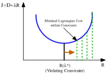
Chapter 2. Constrained Optimization Problems : Principles and Applications
R(λ*) (Violating Constraint)
R J=D+λR
Minimal Lagrangian Cost wit hin Const raint
Figure 2.4: For each independent source, moving the violated value to boundary value achieves minimal Lagrangian cost based on independent and convex properties.
The violated inequalities can be adjusted based on the following two assumptions in video domain:
Independency
Each source signal is independent of others. As a result, a violated source can be adjusted to boundary value to satisfy the constraint without a¤ecting rate-distortion curves of other sources.
Convexity
Each source has one and only one minimal Lagrangian cost operation point based on convexity. Any violated source can be adjusted to boundary value of the constraint to achieve the corresponding constrained local minimum as Figure 2.4.
According to the above assumptions and KKT conditions, if Rk = 0, k 2 H for
several source set H, then uk = 0 for k 2 T = fN Hg, then the original problem becomes min N X k=1 Dk(Rk); s:t: (1) N P k=1 Rk= RN (2)Rk = 0 f or k2 H ) min N X k2T Dk(Rk); s:t: N X k2T Rk = RN
and the solution becomes
D0k(Rk) = | {z } Equal slope for k 2 N nH; where N X k2T Rk = RN
Chapter 2. Constrained Optimization Problems : Principles and Applications
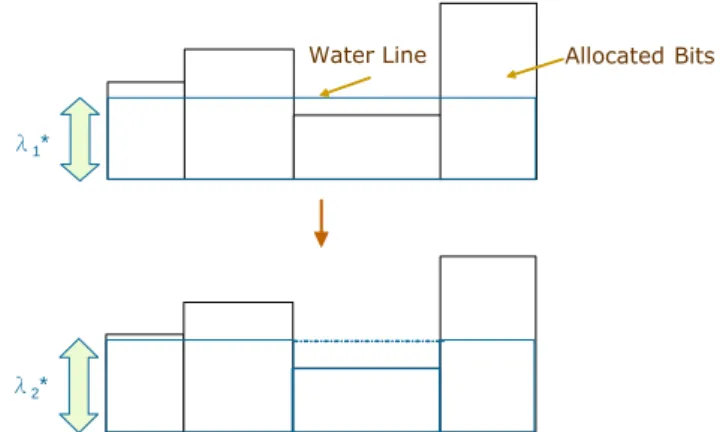
1*
2*
Allocated Bits Water Line
Figure 2.5: Illustration of water …lling principle.
That is, the optimal solution includes the following steps:
1. Ingore the inequality constraints and bring constant slope into practice.
2. If all constraint are satis…ed then the optimal solution is achieved. Otherwise, adjusting the violated constraints by moveing them to the boundary values and no more optimization operations for them.
3. Update the equality constraint.
4. Repeat step 1, 2, 3 until the optimal solution is achieved or there is no suitable solution for current constrained problem.
A graphic illustration of the solution is shown in Figure 2.5, and it is commonly called a water …lling principle.
2.3.2
Optimization Problems with Single Constraint
In [6], a theorem is proposed to solve the budget constrained problem that for any real positive number , the Lagrange multiplier, if the mapping x (i) for i = 1; 2; :::; n minimizes
n
X
i=1
dix(i)+ rix(i)
then it is also the optimal solution to the problem min n X i=1 dix(i), s:t: n X i=1 rix(i) Rt
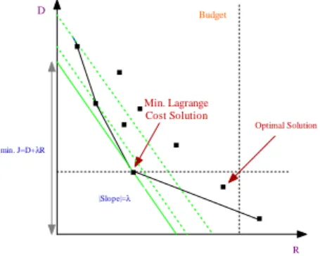
Chapter 2. Constrained Optimization Problems : Principles and Applications D R Budget Min. Lagrange Cost Solution Optimal Solution |Slope|=λ min. J=D+λR
Figure 2.6: Illustration of optimization solution by minimal Lagrangian cost.
where D( ) = n X i=1 dix (i) n X i=1 dix(i), s:t:Rt= R( ) = n X i=1 rix (i)
That is, referring to as the slope (Figure 2.6), for a …xed , we can obtain the best possible solution that meets the budget constraint Rt = Rtotal. And the
is needed to iteratively change by bisection search algorithm [6][10] until we …nd the multiplier , such that the total number of used bits meets the original budget constraint, R( ) = Rtotal, within a convex hull approximation.
Therefore, we can transform the original constrained problem to unconstrained problem, and the solution by this constant slope algorithm is optimal for rate distortion trade-o¤. For example, the typical rate control problem is de…ned to minimize the total distortion
n
P
i=1
Di(Q1; Q2; :::; Qi), where Qi 2 fq1; q2; :::; qNg, subject to the total
rate/budget constraint Rtotal as follows:
min n X i=1 Di(Q1; Q2; :::; Qi); s:t: n X i=1 Ri(Q1; Q2; :::; Qi) Rtotal
and the optimal solution is equal to …nding Q , and to minimize J (Q; ) = n X i=1 Ji(Q1; Q2; :::; Qi); where Ji(Q1; Q2; :::; Qi) = Di(Q1; Q2; :::; Qi) + Ri(Q1; Q2; :::; Qi)
such that J (Q ; ) J (Q; ) and R( ) = Rtotal.
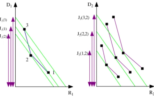
tem-Chapter 2. Constrained Optimization Problems : Principles and Applications 2 3 1 J1(2) J1(1) J1(3) R1 D1 J2(1,2) J2(2,2) J2(3,2) R2 D2
Figure 2.7: Di¤erent quantizer choice for frame 1 leads to di¤erent R-D curve of frame 2, also the solution of minimal lagrangian cost to dependent problem.
poral redundancy in video coding, the quality of previous coded units will impacts the coding e¢ ciency of the following coding units. That is, the sum of minimal Lagrangian cost at each individual stage will not always result in the optimal solution, as Figure 2.7 [7]. Song et al: assumed the dependency relationship between sub-GOPs and propose a real-time system to optimize low-bitrate constrained problem with frame skipping, where the Lagrange multiplier and frames to be encoded for each sub-GOPs are pre-decided [11]. Schuster et al: also developed an MINMAX distortion criterion based on Lagrangian method to solve the minimum rate subject to each source distortion constrained dependent problem [9].
In order to solve this dependent problem, the Viterbi algorithm with Lagrangian cost is applied and we will introduce it in section 2.3.2.1.
2.3.2.1 Viterbi Algorithm for Dependent Problems
Viterbi algorithm [2] is a trellis-based forward dynamic programming procedure which iteratively determines possible shortest paths and prunes out non-optimal paths stage by stage.
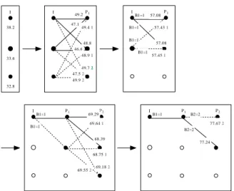
For each stage, a node is an operating point of a quantizer, and a growing branch is connected from node at the previous stage to node at the current stage with corre-sponding Lagrangian cost J = D + R. The optimal solution is the path of minimal Lagrangian cost from the beginning stage to the end stage for a speci…c . When increases, the optimal path is tend to smaller the total coding bits, and vice versa. Still, we have to iteratively …nd by bisection search until R( ) = Rtotal.
Chapter 2. Constrained Optimization Problems : Principles and Applications I 38.2 33.6 32.8 I 49.2P1 47.1 49.41 48.8 46.6 48.91 49.72 47.52 49.92 I P1 B1=1 B1=1 B1=1 B1=1 57.08 57.431 57.08 57.451 I P1 B1=1 B1=1 P2 69.29 68.39 69.641 68.751 69.182 69.552 I P1 B1=1 P2 77.24 B2=2 B2=2 77.672
Figure 2.8: Illustration of Viterbi algorithm with minimal Lagrangian cost path in IBBP case.
Ramchandran et al: applied VA algorithm with Lagrangian cost and propose prun-ing rules based on monotonicity property, as Figure 2.8 [7]. Assume the quantizer grades ordered from …nest to coarsest, for any 0, there exists monotonicity prop-erty that for i i0
J2(i; j) < J2(i 0
; j)
where quantizer j of frame 2 is dependent on quantizer i of frame 1. Afterwards, the pruning conditions based on monotonicity property are used to eliminate suboptimal operating points:
Pruning Condition 1
If J1(i) + J2(i; j) < J1(i0) + J2(i0; j), for any i < i0, then (i0; j) can be pruned
out.
Pruning Condition 2
If J2(i; j) < J2(i; j0), for any j < j0, then (i; j0) can be pruned out.
Pruning Condition 3
According to monotonicity property and pruning conditions, if J1(i) < J1(i0) for
i < i0, then state node i0 can be pruned (for I frames).
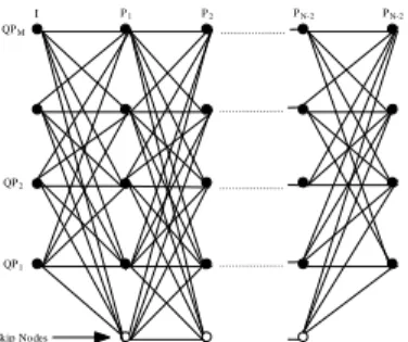
In [4], Liu et al: also improved VA by considering frame skipping situation, as Figure 2.9 [4], and assumed monotonicity property with frame skipping brings into being for
Chapter 2. Constrained Optimization Problems : Principles and Applications I QPM QP1 QP2 P1 Skip Nodes P2 ... ... ... ... ... PN-2 PN-2
Figure 2.9: VA with skip nodes
any 0,
J (i; sij; j) J (i0; si0j; j); if i i0
J (i; sij; j) J (i; sij0; j0); if j j0
J (i; sij; j) J (i0; si0j0; j0); if i i0; j j0
where sij represents skipped frame reconstructed from forward coding frame with
quantizer i and backward coding frame with quantizer j. Also, the new pruning rules are:
Pruning Condition 4
If J (i) + J (i; sij; j) + J (i; j) J (i 0
) + J (i0; si0j; j) + J (i0; j), for i < i0 then branch
J (i0; s
i0j; j) can be pruned out.
Pruning Condition 5
If J (i; sij; j) + J (i; j) J (i; sij0; j0) + J (i; j0), for j < j0 then branch J (i; sij0; j0)
can be pruned out.
2.3.2.2 Viterbi Algorithm for Independent Problems
Though dynamic programming can apply to …nding the optimal solution to depen-dent problems, it takes too much computation considering frame-to-frame dependency. In order to reduce complexity, solution to dependent problem usually reduced to in-dependent problem; that is, take rate constrained problem for example, the problem formulation becomes min n X i=1 Di(Qi); s:t: n X i=1 Ri(Qi) Rtotal
Chapter 2. Constrained Optimization Problems : Principles and Applications The solution to independent problem only focuses on …nding the minimal La-grangian cost at current stage despite of the e¤ect of other stages.
2.4
Complexity Comparison
Table 2.1 lists the complexity of two di¤erent dynamic programming procedures, integer programming and Lagrangian cost based Viterbi algorithm, for the optimal solution to optimization problems with multiple constraints.
In the dependent case, these two DP algorithms both grow exponentially. However, in the independent case, Lagrange multiplier method can reduce complexity enormously by selecting the minimal Lagrangian cost node at each stage, though it still has to iteratively re…ne the value of Lagrange multiplier; as for integer programming, because it does not have a independent form, the complexity remains the same.
Besides, owing to each constraint corresponding to a Lagrange multiplier, and the optimal solution by Lagrangian method needs to solve each Lagrange multiplier iter-atively, integer programming for multiple constrained case is better than Lagrangian optimization for lower complexity; however, as for singular equality constrained prob-lem, Lagrangian optimization is more suitable for only one Lagrange multiplier to be solved, and a fast algorithm can be developed based on independency assumption. The following lists the de…nition of variables:
N : Number of Coding Units
M : Number of Operating Modes per Coding Units C : Number of Constraints
T : Number of Test Points per Lagrange Multiplier
Table 2.1: Complexity comparison between DP Integer Programming Lagrange Multiplier
Optimal Convex Approx. NM (Dependent) TCNM (Dependent)
CHAPTER 3
Related Works
In this chapter, we will introduce how related works applied the optimization methods described in previous chapter into their constrained problem. Also, the di¤erence between related works and our proposed problem is listed in the end.
3.1
KKT Conditions
Wang et al: used Karush–Kuhn–Tucker Conditions to solve long-term distortion con-strained problem for I frames [12]; the fomulation and algorithm for their problem are in the following:
P roblem F ormulation
Let # be a set of quantizers and let Dmin and Dmaxbe the lower and upper bounds
of the distortion for each source sample. Find Q = (Q1; Q2; :::; Qn), with Qi 2 #
for i = 1; 2; :::; n, where n is the number of source samples, such that Q = arg min Q2# n X i=1 Ri(Qi)
Chapter 3. Related Works s:t: (1)Dmin Di(Qi) Dmax; i = 1; 2; :::; n (2) n P i=1 Di(Qi) Dtotal = (Dmin+Dmax) 2 n Algorithm
1. Consider the original optimization problem with multiple constraints as an equivalent problem with a total “distortion budget”, Dtotal= (Dmin+D2 max) n.
2. Apply the Lagrangian method to solve the problem with Dmin = 0 and
Dmin = 1. The result is the constant slope solution with optimal 0 and
corresponding Q0, such that Pn i=1
Di(Qi) Dtotal. The approximation is due
to the fact that the operational rate-distortion function is a discrete function. 3. Impose the distortion constraints. The quantization found in the previous step is the optimal solution that minimizes total bit rate for a given total distortion. For any frame i, the constraint condition Dmin Di(Q0i) Dmax
may be violated. Depending on the value of Di(Q0i), frames are divided into
three groups:
(a) If Di(Q0i) < Dmin, the constant slope solution for this frame is not
admissible. In this case, we need to replace Q0
i by an admissible Qi
such that Di(Qi) Dmin.
(b) Similarly, if Di(Q0i) Dmax, replace Q0i by an admissible Qi such that
Di(Qi) Dmax.
(c) If Dmin Di(Q0i) Dmax, the constant slope solution Di(Q0i) does
not violate the distortion constraints, but, due to the changes of the operating points of the frames in the other two groups, the Q values for this group cannot be …nalized at this stage.
4. Initialize the next iteration. Let the number of frames in the above three groups be Nmin, Nmax, and Nmid, respectively. If Nmin = Nmax = 0, then
the constant slope solution found in Step 2 is also the solution to the given distortion-constrained problem. Otherwise, performs
N Nmid
Dtotal Dtotal NminDmin NmaxDmax
Chapter 3. Related Works algorithm and the Q found at this iteration is the approximated solution to the given distortion-constrained problem.
3.2
Viterbi Algorithm with Lagrangian Cost
Liu et al: applied Viterbi algorithm with Lagrangin cost to solving the spatial quality (QP) selection, temporal resolution (frame rate) optimization problem in [4], where they use MCI as a temporal interpolation method to reconstruct skipped frames. The formulation and algorithm for their problem are in the following:
P roblem F ormulation
Let # be a set of quantizers ranging from Qminto Qmax. Find Q = (Q1; Q2; :::; Qn),
with Qi 2 # for i = 1; 2; :::; n, where n is the number of source samples, and …nd S = (S1; S2; :::; Sn) with Si 2 [0; 1], where Si = 0 represents current frame is
skipped, Si = 1 represents current frame is encoded; the maximal number of
successive skipping frame Smax= 2, such that
(Q ; S ) = arg min Q2#;S2[0;1] N X i=1 Di(Q; S) = N X i=1 fDi(Qi)j(Si = 1) + Di(Qi)j(Si = 0)g s:t: N X i=1 Ri(Q; S) = N X i=1 Ri(Qi)j(Si = 1) Rbu dg et where S = [S1; S2; :::; SN]; Si 2 [0; 1]; i = 1; :::; N # = [Q1; Q2; :::; QN]; Qi 2 [Qmin; Qmax]; i = 1; :::; N Algorithm
1. Initialize the value of :
2. Calculate for the …rst frame, which is an I-frame, for every QP value within the range i 2 [Qmin; Qmax], as shown in Figure 3.1 (a).
3. Prune unquali…ed I-nodes according to the monotonicity property as shown in Figure 3.1 (b).
4. Grow the trellis to Stage 2 by coding the …rst P-frame with all QP values. The skip node is reserved as shown in Figure 3.1 (c).
Chapter 3. Related Works I I I P1 Skip Node I P1 I P1 P2 I P1 P2 (a) (b) (c) (d) (e) (f) I P1 P2 P3 I P1 P2 P3 I P1 P2 P3 (g) (h) (i)
Figure 3.1: Illustrative example of the Viterbi algorithm with skip nodes.
shown in Figure 3.1 (d).
6. Grow the trellis to one more stage. The skipped frame in the previous stage is reconstructed by the neighboring reference frames coded with selected QPs as shown in Figure 3.1 (e).
7. Prune at Stage 3 based on the monotonicity property, i.e., Rules 1 and 2 for pruning the third coded frames, Rules 3 and 4 for pruning previous skipped frames. The skip node at Stage 3 is reserved as shown in Figure 3.1 (f).
8. Similar to Step 4, grow trellis to Stage 4 as shown in Figure 3.1 (g).
9. Prune paths that have more successive skipped frames than Smax as shown in
Figure 3.1 (h).
10. Similarly to Step 7, pruning is performed based on the monotonicity property as shown in Figure 3.1 (i).
11. Repeat Step 8–10 until the last frame. Update and return to Step 2. 12. Stop when converges.
3.3
Variable Frame Rates Encoding
Song et al. proposed a rate control mechanism for low-bit-rate video via variable-encoding frame rates in [4]. In order to implement this variable frame rate variable-encoding under real time environment, they divide each gop into 8 sub-GOPs with size=12 for complexity issue and de…ne the value of each Lagrange multiplier for each sub-GOP
Chapter 3. Related Works under the consideration of dependency relationship between sub-GOPs. The proposed algorithm consist of two parts:
1. Frame-Rate Control
Decide the frame rate (number of encoded frames) and encoded frame positions for each sub-GOP before encoding based on the histogram of di¤erence image. 2. Bit Allocation
Use gradient search method to obtain the optimal QP setting for individual frame encoding in each sub-GOP, such that the following problem statement is satis…ed. P roblem F ormulation Determine q!m, m=1,2,...,M to minimize M X m=1 (Dm( ! qm) + wqEm( ! qm)) s:t: M X m=1 rm( ! qm) Bsubgop M
where q!m = (qm;1; qm;2; :::; qm;Nm) is the quantization parameter vector for the mth
sub-GOP, and
Nm : encoded frame number of the mth sub-GOP;
rm( !
qm) : assigned number of bits for the mth sub-GOP;
M : number of sub-GOPs in a GOP; Nsubgop : total frame number of a sub-GOP;
Ngop : total frame number of a GOP;
wq : weighting factor for abrupt quality change and ‡ickering;
di(q1; q2; :::; qi) : distortion measure for the ith frame;
ri(q1; q2; :::; qi) : allocated bit rates for the ith frame;
and Dm( ! qm) = 1 Nm Nm X i=1 di(q1; q2; :::; qi); Em( ! qm) = 1 Nm Nm X i=1 (di(q1; q2; :::; qi) di 1(q1; q2; :::; qi 1))2 Dm( !
qm)represents the distortion measure of encoded frames, and Em( !
qm)represents
the distortion variance measure of two successive encoded frames; besides, wq is a
Chapter 3. Related Works
Table 3.1: Comparison among the proposed problem and related works
Author Thesis Wang et al: [12] A. Ortega [5]
Constraints Rate, Distortion(Multiple) Distortion(Multiple) Bu¤er(Multiple)
Frame Skipping Y N N
Recovery Method Frame Copy NA NA
Frames to be Encoded Unknown Pre-Decided Pre-Decided
Lagrange Multiplier Value Bisection Search Bisection Search Bisection Search
Proposed Algorithm VA KKT Conditions KKT Conditions
Author Schuster et al:[9] Ahmad et al:[1]
Constraints Distortion(Multiple) Perceptual Quality(Multiple)
Frame Skipping N N
Recovery Method NA NA
Frames to be Encoded Pre-Decided Pre-Decided
Lagrange Multiplier Value Bisection Search (Dmax) Bisection Search
Proposed Algorithm DP KKT Conditions
Author Liu et al: [7] Song et al: [11]
Constraints Rate Rate
Frame Skipping Y Y
Recovery Method Temporal Interpolation Frame Copy
Frames to be Encoded Unknown Pre-Decided
Lagrange Multiplier Value Bisection Search Pre-Decided
Proposed Algorithm VA Gradient Search
in their experiments.
After de…ning the penalty function for the mth sub-GOP as
Pm( ! qm) = m X i=1 ri( ! qi) m Bsubgop
and applying the pre-de…ned Lagrange multiplier m, the above constrained
prob-lem becomes to minimize the following unconstrained function
m( ! qm; m) = Jm( ! qm) + mmaxf0; Pm( ! qm)g; for m = 1; 2; :::; M where Jm( ! qm) = Dm( ! qm) + wqEm( ! qm)
and a gradient search method was used to …nd the optimal solution.
3.4
Comparison
In order to understand the di¤erences between the proposed quality- and rate-constrained problem and other constrained problems, we compare and list several features in Table 3.1.
From the above table, we can clearly observe that our problem is di¤erent from the others and our problem is di¢ cult for having variable multiple constraints, uncertain to
Chapter 3. Related Works number of skipped frames, and the dependent relation between frames to be skipped and frames to be encoded. Besides, The best method of getting the optimal solu-tion to our constrained problem is to use integer programming instead of Lagrangian optimization.
CHAPTER 4
Experiments and Analyses
In this chapter, we implement the integer programming to solve our quality- and rate-constrained problem, and analyze the optimal solution path; then, in order to reduce complexity, we propose a simple heuristic solution based on independent relationship and successive re…nement assumption. Figure 4.1 shows our experiment procedures; the experiment settings, experiment results and observations for each experiment are described in each section. We use jm 12.3 and CIF format with 37~39 psnr constraints in all experiments.
4.1
Optimal Solution Analyses
We implement the integer programming algorithm to solve our constrained problem, and observe the R-D data from the view of MSE, optimal path, and then propose the concept of dominant lines.
Chapter 4. Experiments and Analyses
4.1.1
MSE Weighting E¤ect
Setting:
Sequence Akiyo, Mobile
Algorithm Integer Programming Total Frame 8
Experimental Group Coded Frame MSE, Copy Frame MSE, Total MSE with Frames to be Encoded=7
Control Group Coded Frame MSE, Copy Frame MSE, Total MSE with Frames to be Encoded=2
Observation
Copy frame MSE e¤ect:
From Figure 4.2 and 4.3, we can clearly observe the copy frame MSE weights overwhelmingly compared to the coded frame MSE.
Variation line in local view, horizontal line in global view:
Though the coded frame MSE varies among di¤erent coding bit range in Figure 4.2 (b) and 4.3 (b), the overall MSE looks like horizontal lines for copy frame MSE e¤ect.
Larger MSE gap with more frame skipped:
From Figure 4.2 (a), 4.4 (a) and Figure 4.3 (a) ,4.4 (b), the gap between di¤erent coding frame selections is larger while more frames are skipped.
Unobvious dominant lines in static sequence:
There does not exist obvious horizontal dominant lines in static sequence, how-ever, the gap among di¤erent coding frame selections is minor with less frame
Complexity Is s ue Frame Selection Effect
Dominant Lines Optimal Path Analys es
Total Frame MSE Coded Frame MSE Analys es Copy Frame MSE
Optimal Solution
Independent Heuristic Algorithm
Two Frame Selection Methodologies
Successive Refinement Mechanism
Chapter 4. Experiments and Analyses AKIYO K Bits 26 27 28 29 30 Total MSE 340 360 380 400 420 440 460 480 Coded Frame=1,2 Coded Frame=1,3 Coded Frame=1,4 (a) AKIYO K Bits 26 27 28 29 30
Coded Frame MSE
20 21 22 23 24 25 Coded Frame=1,2 Coded Frame=1,3 Coded Frame=1,4 AKIYO K Bits 26 27 28 29 30 Copy Frame MSE 300 320 340 360 380 400 420 440 460 Coded Frame=1,2 Coded Frame=1,3 Coded Frame=1,4 (b) (c)
Figure 4.2: Total MSE(a), coded frames MSE(b) and copy frames MSE(c) in Akiyo when encoding 2 frames.
skipped as Figure 4.2 (a) and 4.4 (a).
Obvious dominant lines in motion sequence:
There exists a dominant line for each di¤erent total coding frame in motion sequence as Figure 4.3 (a) and 4.4 (b).
Remarks
Because the copy frame MSE weights overwhelminly compared to coded frame MSE, choosing the correct combination of coding frames is more important than allocating bits among these frames; besides, since the gap between di¤erent coding frame selec-tions is large and there exists a dominant line for each di¤erent total coding frames, we can reduce the original multiple constraints dependent problem to independent problem by always …nding the corresponding dominant line of current encoding frame numbers, which is the basic idea of our heuristic solution.
Chapter 4. Experiments and Analyses MOBILE K Bits 340 360 380 400 420 Total MSE 9000 10000 11000 12000 13000 Coded Frame=1,2 Coded Frame=1,3 Coded Frame=1,4 Coded Frame=1,5 Coded Frame=1,6 Coded Frame=1,7 Coded Frame=1,8
Dominative Line with Number of Coded Frame=2
(a) MOBILE K Bits 340 360 380 400 420 Coded Frame MSE 16 17 18 19 20 21 22 23 24 Coded Frame=1,2 Coded Frame=1,3 Coded Frame=1,4 Coded Frame=1,5 Coded Frame=1,6 Coded Frame=1,7 Coded Frame=1,8 MOBILE K Bits 340 360 380 400 420 Copy Frame MS E 9000 10000 11000 12000 13000 Coded Frame=1,2 Coded Frame=1,3 Coded Frame=1,4 Coded Frame=1,5 Coded Frame=1,6 Coded Frame=1,7 Coded Frame=1,8 (b) (c)
Figure 4.3: Total MSE(a), coded frames MSE(b) and copy frames MSE(c) in Mobile when encoding 2 frames.
AKIYO K bits 34.0 34.5 35.0 35.5 36.0 36.5 37.0 Total MSE 90 95 100 105 110 115 120 125 Skipped Frame=1 Skipped Frame=2 Skipped Frame=3 Skipped Frame=4 Skipped Frame=5 MOBILE k bits 840 860 880 900 920 940 Avg. MSE 620 640 660 680 700 720 740 Skip 1 Skip 2 Skip 3 Skip 4 Skip 5 Skip 6 Skip 7
Dominative Line with Number of Coded Frame=7
(a) (b)
Chapter 4. Experiments and Analyses AKIYO K Bits 26 28 30 32 34 36 Total MSE 100 200 300 400 500
Number of Encoding Frame=2 Number of Encoding Frame=3 Number of Encoding Frame=4 Number of Encoding Frame=5 Number of Encoding Frame=6 Number of Encoding Frame=7 Optimal Path (a) MOBILE K Bits 300 400 500 600 700 800 900 Total MSE 0 2000 4000 6000 8000 10000
12000 Number of Encoding Frame=2Number of Encoding Frame=3 Number of Encoding Frame=4 Number of Encoding Frame=5 Number of Encoding Frame=6 Number of Encoding Frame=7 Optimal Path FOOTBALL K Bits 200 300 400 500 600 700 Total MSE 0 2000 4000 6000 8000 10000
Number of Encoding Frame=2 Number of Encoding Frame=3 Number of Encoding Frame=4 Number of Encoding Frame=5 Number of Encoding Frame=6 Number of Encoding Frame=7 Optimal Path
(b) (c)
Figure 4.5: Optimal path from low bit budget to high bit budget of (a)Akiyo, (b)Mobile, (c)Football.
4.1.2
Optimal Path Analyses
Setting:
Sequence Akiyo, Mobile, Football Algorithm Integer Programming Total Frame 8
Observation
Optimal path is a stairway-like curve:
Figure 4.5 shows the optimal path of (a)Akiyo, (b) Mobile, (c) Football when coding bits range from low to high. The optimal path is a stairway-like curve, which means number of frames to be encoded and coding frame selection should be di¤erent to optimize our constrained problem while the available bit budget changes.
Optimal path chooses di¤erent total coding frames interactively in static se-quence:
Chapter 4. Experiments and Analyses AKIYO K Bits 26 27 28 29 30 31 32 Total MSE 300 350 400 450 500
Number of Encoding Frame=2 Number of Encoding Frame=3 Number of Encoding Frame=4 Optimal Path Coded Frame=1,4 Coded Frame=1,2,3 Interlacing MOBILE K Bits 500 600 700 800 Total MSE 0 2000 4000 6000 8000
Number of Encoding Frame=2 Number of Encoding Frame=3 Number of Encoding Frame=4 Number of Encoding Frame=5 Number of Encoding Frame=6 Number of Encoding Frame=7 Optimal Path
Coded Frame=1,2,4,6,7
Coded Frame=1,3,5,7 Same Coded Frame Selection, Different Bit Allocation
(a) (b) FOOTBALL K Bits 300 350 400 450 500 Total MSE 3000 4000 5000 6000 7000
8000 Number of Encoding Frame=3 Number of Encoding Frame=4 Number of Encoding Frame=5 Optimal Path Stairway-Like Curve FOOTBALL K Bits 200 300 400 500 600 700 Total MSE 0 2000 4000 6000 8000 10000
Number of Encoding Frame=2 Number of Encoding Frame=3 Number of Encoding Frame=4 Number of Encoding Frame=5 Number of Encoding Frame=6 Number of Encoding Frame=7 Optimal Path
Overlapped
(c) (d)
Figure 4.6: Overall distortion may interlace in static sequence like Akiyo(a); the correct Qp selection for each coding frame may not only reduce coding bits but also reduce overall distortion(b); while available bit budget decreases, the optimal solution may choose di¤erent frames to be encoded instead of skipping another frame immedi-ately(c).
of total coding frames may increase, as the interlacing part in Figure 4.6 (a); however, this situation would not occur in motion sequence such as Football and Mobile for Frame copy MSE weights largely.
Encoding more bits does not always results in smaller distortion:
Not always using more bits results in smaller distortion, as Figure 4.6 (b). Be-cause skipped frame makes temporal dependency decrease and the frame copy e¤ect, even we allocate bits among the same selected frames, the correct Qp set-ting for each frame sometimes not only reduce coding bits but also reduce overall distortion.
Choosing another coding frame combination is better than skipping another frame immediately:
In Figure 4.6 (c) we can observe the clear stair-way curve, which means the optimal path should select another frame combination instead of choosing another frame to be skipped immediate when bit budget decrease.
Chapter 4. Experiments and Analyses AKIYO k bits 26 28 30 32 34 36 38 40 Total MSE 100 150 200 250 300 350 400 Coded Frame=1,6 Coded Frame=1,3,6 Coded Frame=1,3,5,7 Coded Frame=1,3,5,6,7 Coded Frame=1,3,4,5,6,7 Coded Frame=1,2,3,4,5,6,7 Independent (a) MOBILE k bits 400 500 600 700 800 Total MSE 2000 4000 6000 8000 Coding Frame=1,5 Coding Frame=1,3,6 Coding Frame=1,3,5,7 Coding Frame=1,2,4,6,7 Coding Frame=1,2,3,5,6,7 Coding Frame=1,2,3,4,5,6,7 Independent FOOTBALL k bits 100 200 300 400 500 600 700 800 Total MSE 0 2000 4000 6000 8000 10000 12000 Coded Frame=1,5 Coded Frame=1,4,7 Coded Frame=1,3,5,7 Coded Frame=1,3,5,7,8 Coded Frame=1,3,5,6,7,8 Coded Frame=1,3,4,5,6,7,8 Independent (b) (c)
Figure 4.7: Dominative lines of di¤erent total number of coded frames.
Selecting another frame to be skipped immediately for complexity issue when less frame skipped:
From Figure 4.6 (d), the bit range of number of coded frame=5 is overlapped with the bit range of number of coded frame=4; however, the bit range of number of coded frame=3 is not overlapped with the bit range of number of coded frame=2. That is, when available bit decreases, to select a frame to be skipped is a good choice with less frame skipped, but it is better to select another coding frame combination with more frame skipped.
Remarks
The optimal solution to our proposed constrained problem is to use dynamic pro-gramming. However, in Figure 4.5, each line represents a coding frame combination, e.x. when enocding 3 frames, 1-4-5, among total 8 frames, the optimal solution chooses di¤erent coding frame combinations to adapt di¤erent bit budget constraint and it must be iteratively solved. Therefore, we want to reduce complexity from dependent problem to independent problem, which becomes to …nd each dominate line among di¤erent total number of coded frames as Figure 4.7.
Chapter 4. Experiments and Analyses I I I P1 I P1 Jmin I P1 P2 I P1 P2 Jmin I P1
out of quality constraint Skip
Node
Figure 4.8: Illustration of heuristic solution for independent problem with multiple constraints by Viterbi algorithm.
4.2
Proposed Heuristic Solution
Figure 4.8 illustrates the algorithm ‡ow, and described in the following: 1. Set = 0:
2. Choose the quantization parameter operation point of I frame where lagrangian cost J = D + R is minimal.
3. Grow the branch from the minimal node of this stage to next stage with QPnext =
QPcurrent 5, and prune out the node with unsatis…ed quality constraint.
4. Select the operation point with minimal lagrangian cost among current stage, and repeat 3, 4 until to the end stage.
5. Increase gradually until any more increase to will result in skipping another frame.
4.2.1
Coding Frame Selection Methodologies
Setting:
Sequence Akiyo, Mobile, Football Total Frame 8
Experimental Group Two Coding Frame Selection Methodology with Heuristic Algorithm Control Group Non-Coding Frame Selection Methodology with Heuristic Algorithm
Chapter 4. Experiments and Analyses 1 2 3 4 5 6 7 8 1 1 1 4 4 4 7 7 Original frame Candidate combination ) 4 6 ( ) 4 5 ( ) 1 3 ( ) 1 2 ( − + − + − + −
Figure 4.9: Illustration of methodology 1.
1 2 3 4 5 6 7 8 1 1 1 4 4 4 7 7 )} 4 6 ( ) 4 5 ( ) 1 3 ( ) 1 2 {( − + − + − + − )} 7 8 ( ) 4 7 ( ) 1 4 {( − + − + − + Original frame Candidate combination
Figure 4.10: Illustration of methodology 2.
The result is in Figure 4.11
1. Suppose there are total i frames in the pre-analysis bu¤er, and j skipped frames to be chosen, the overall candidates are i!(i j)!i! combinations. This methodology is towards to …nd the minimal sum of di¤erence between coding frame and copy frame. As Figure 4.9, suppose there are 8 frames in the bu¤er, and we are going to choose frame 1, 4, and 7 as coding frames.
2. Almost the same as methodology 1, excepts that this methodology also considers the di¤erence between coding frames. Figure 4.10 shows a candidate combination. Observation
In static sequence, methodology 1 and 2 doesn’t have too much performance di¤erence.
Methodology 1 obtains smaller MSE curve than methodology 2 in motion se-quence.
These two methodology doesn’t perform too bad compared with independent R-D curve.
Remarks
Once we know how many coded frames available to encode, we can use these two methodologies to choose which frames to be encoded and reduce complexity compared
Chapter 4. Experiments and Analyses AKIYO K Bit 28 30 32 34 36 Total MSE 100 150 200 250 300 Independent Copy Total (a) MOBILE K Bit 300 400 500 600 700 800 900 Total MSE 0 2000 4000 6000 8000 Independent Copy Total FOOTBALL K Bit 300 400 500 600 Total MSE 0 2000 4000 6000 8000 Independent Copy Total (b) (c)
Figure 4.11: Comparison among proposed heuristic solution, methodology 1 and methodology 2 in Akiyo (a), Mobile(b) and Football(c).
Skipped Frame Coding Frame Iteration 2 Iteration 1 Iteration 3 Iteration 4 1 2 3 4 5 6 7 8
Figure 4.12: Illustration of successive re…nement.
to independent solution, though it still needs to try i!(i j)!i! combinations, which means once the window size increases, the calculation will also increases exponentially.
4.2.2
Successive Re…nement
De…nition of Successive Re…nement
Chapter 4. Experiments and Analyses AKIYO K Bit 28 30 32 34 Total MSE 100 120 140 160 180 200 220 240 260 Independent Independent SR. (a) AKIYO K Bit 28 30 32 34 36 Total MSE 100 150 200 250 300 Independent Copy Copy SR. AKIYO K Bit 28 30 32 34 Total MSE 100 150 200 250 300 Independent Total Total SR. (b) (c)
Figure 4.13: Comparison among proposed heuristic solution and its successive re-…nement(a), methodology 1 and its successive re…nement(b), methodology 2 and its successive re…nement(c) in Akiyo.
then frame i must be skipped …rst, as Figure 4.12. Setting:
Sequence Akiyo, Mobile, Football Total Frame 8
Experimental Group Successive Re…nement Control Group Non-Successive Re…nement
The result for Akiyo is in Figure 4.13, for Mobile in Figure 4.14 and for Football in Figure 4.15
Observation
No matter which coding frame selection methodology is used, the di¤erence between successive re…nement R-D curve and non-successive re…nement R-D curve is minor.
Remarks
While using successive re…nement, the complexity can reduce from exponential increasing to linear increasing.
Chapter 4. Experiments and Analyses MOBILE K Bit 400 500 600 700 800 Total MSE 0 2000 4000 6000 8000 Independent Independent SR. (a) MOBILE K Bit 300 400 500 600 700 800 900 Total MSE 0 2000 4000 6000 8000 10000 Independent Copy Copy SR. MOBILE K Bit 300 400 500 600 700 800 900 Total MSE 0 2000 4000 6000 8000 10000 Independent Total Total SR. (b) (c)
Figure 4.14: Comparison among proposed heuristic solution and its successive re-…nement(a), methodology 1 and its successive re…nement(b), methodology 2 and its successive re…nement(c) in Mobile.
4.3
Proposed Rate Control Mechanism
As Figure 4.16, we propose an iterative successive re…nement mechanism to solve the original problem in the independent way. The main idea of the algorithm is to decide which frames to be encoded at the …rst place for MSE of di¤erent copy frames com-binations are huge; then we can allocate available bits among these chosen frames to encode and achieve the objective of total minimal distortion. Suppose that there is a R-D model which can estimate the needed coding bits, the rate control algorithm is the following:
Step 1 :
Use the r-d model to calculate the needed coding bits while encoding pre-selected frames at distortion=Dmax. If the required bits are smaller than available bits, go to
Step 3, else go to Step 2. Step 2 :
Use frame selection methodology to select a frame to be skipped with successive re…nement mechanism, and go to Step 1.
Chapter 4. Experiments and Analyses FOOTBALL K Bit 200 300 400 500 600 700 Total MSE 0 2000 4000 6000 8000 Independent Independent SR. (a) FOOTBALL K Bit 200 300 400 500 600 700 Total MSE 0 2000 4000 6000 8000 Independent Copy Copy SR. FOOTBALL K Bit 200 300 400 500 600 700 Total MSE 0 2000 4000 6000 8000 Independent Total Total SR. (b) (c)
Figure 4.15: Comparison among proposed heuristic solution and its successive re-…nement(a), methodology 1 and its successive re…nement(b), methodology 2 and its successive re…nement(c) in Football.
Start Set # of Skipped Frame
Snumber=0
Select Which Frames to be Encoded Estimate Coding Bit Bestimateby
R-D Model with Distortion=Dmax
If Bestimate<= Rt
Nskip=Nskip+1
No
Allocate Bit Budget Among Selected Frames to Minimize
Overall Distortion End Stage 1: Frame Selection Stage 2: Bit Allocation Yes
Figure 4.16: Proposed algorithm ‡owchart. At the …rst stage to decide which frames to be encoded; to allocate bit among selected frames at the second stage.
Chapter 4. Experiments and Analyses Step 3 :
Since skipped frames are out of the optimization target, we can simply allocate available bits among those selected coding frames and achieve the goal of minimum overall distortion.
CHAPTER 5
Conclusions and Future Works
In our work, we attempted to solve the quality- and rate-constrained problem and survey di¤erent constrained optimization problem methodologies. After comparing with related works and analyze our problem, we …nd out the best methodology for optimal solution is to use dynamic programming and the optimal path is a stairway-like curve, with huge complexity, the following lists our discoveries:
1. Constrained problems can be solved by dynamic programming. A simple algo-rithm for constrained optimization problem is to …nd the optimal solution among possible data set as integer programming; another commonly used mathematical tool for optimization problems is Lagrangian method, which turns the original constrained problem into unconstrained problem form.
2. For optmization problems with multiple constraints, each constraint correspond-ing to a Lagrangian multiplier, and the optimal solution should be obtained by iteratively adjusting each Lagrangian multiplier according to KKT conditions. As a result, the solution by constrained optimization problem like integer program-ming requires lower complexity than Lagrangian optimization; however, as for the single equality constrained problem, the Viterbi algorithm with Lagrangian
Chapter 5. Conclusions and Future Works cost is commonly used owing to only one Lagrange multiplier variable to be solve, and the modern rate control apply this algorithm to real time system based on independency assumption.
3. According to optimal solution by integer programming for our problem, the op-timal path is a stairway-like curve, which means number of frames to be encoded and coding frame selection should be di¤erent to optimize our constrained prob-lem while the available bit budget changes. Furthermore, as long as more frame skipped, the MSE gap between each rate distortion line of di¤erent coding frame combination is larger; also, the interlacing part among coding bit range of di¤er-ent coding frame combination is getting smaller. From the above observation, it is a good choice to select another frame to be skipped while the available bit bud-get decreases in less frame skipped case for complexity issue, but it should choose another coding frame selection instead of skipping another frame immediately while more frame skipped.
4. In order to reduce complexity and to implement the proposed architecture in a real-time system, we try to develop a heuristic algorithm based on independent assumption and successive re…nement and devide the solution into two stages: 2.1) to …nd which frames to be encoded under rate constraint and distortion constraints;
2.2) to allocate available bit budget among these chosen frames to achieve the objective of minimize total distortion.
The experimental result shows this heuristic solution can reduce complexity ex-ponentially, though it does not achieve a good performance because the optimal path reveals that the encoder should choose di¤erent frames to encode when target rate changes.
Our work is still in its early stage, we plan to extend our investigation in several directions:
1. To survey other adaptive frame skipping methods and continue to research if there exits a better algorithm for our problem.
2. To replace the frame copy with temporal interpolation methodology and analyze the e¤ect.
Chapter 5. Conclusions and Future Works total distortion for real-time systems.
Bibliography
[1] I. Ahmad and J. Luo, “On Using Game Theory to Optimize the Rate Control in Video Coding,”IEEE Transactions on Circuits and Systems for Video Technology, vol. 16, no. 2, Febuary 2006.
[2] J. G. David Forney, “The Viterbi Algorithm,” Proceedings of The IEEE, vol. 61, no. 3, March 1973.
[3] W. Kaplan, “Maxima and Minima with Applications: Practical Optimization and Duality,” Wiley-IEEE, 1999.
[4] S. Liu and C.-C. J. Kuo, “Joint Temporal-Spatial Bit Allocation for Video Cod-ing With Dependency,” IEEE Transactions on Circuits and Systems for Video Technology, vol. 15, no. 1, January 2005.
[5] A. Ortega, “Optimal bit allocation under multiple rate constraints,” IEEE Data Compression Conference (DCC), 1996.
[6] A. Ortega, K. Ramchandran, and M. Vetterli, “Optimal Trellis-Based Bu¤ered Compression and Fast Approximations,”IEEE Transactions on Image Processing, vol. 3, no. 1, January 1994.
BIBLIOGRAPHY [7] K. Ramchandran, A. Ortega, and M. Vetterli, “Bit Allocation for Dependent Quantization with Applications to Multiresolution and MPEG Video Coders,” IEEE Transactions on Image Processing, vol. 3, no. 5, September 1994.
[8] E. C. Reed and J. S. Lim, “Optimal Multidimensional Bit-Rate Control for Video Communication,”IEEE Transactions on Image Processing, vol. 11, no. 8, August 2002.
[9] G. M. Schuster, G. Melnikov, and A. K. Katsaggelos, “A Review of the Minimum Maximum Criterion for Optimal Bit Allocation Among Dependent Quantizers,” IEEE Transactions on Multimedia, vol. 1, no. 1, March 1999.
[10] Y. Shoham and A. Gersho, “E¢ cient Bit Allocation for an Arbitrary Set of Quan-tizers,” IEEE Transactions on Acoustics. Speech. and Signal Processing, vol. 36, no. 9, September 1988.
[11] H. Song and C.-C. J. Kuo, “Rate Control for Low-Bit-Rate Video via Variable-Encoding Frame Rates,” IEEE Transactions on Circuits and Systems for Video Technology, vol. 11, no. 4, April 2001.
[12] K. Wang and J. W. Woods, “MPEG Motion Picture Coding With Long-Term Constraint on Distortion Variation,”IEEE Transactions on Circuits and Systems for Video Technology, vol. 18, no. 3, March 2008.