Boundary Element Analysis and Design in Seepage Problems Using Dual Integral Formulation

(1)

Please cite this paper as follows:

J.-T. Chen, H.-K. Hong and S.-W. Chyuan, Boundary Element Analysis and Design in Seepage

Problems Using Dual Integral Formulation, Finite Elements in Analysis and Design, Vol.17, pp.1-20,

(2)

FINITE ELEMENTS IN ANALYSIS AND DESIGN Finite Elements in Analysis and Design 17 (1994) l-20

Boundary element analysis and design in seepage problems using

dual integral formulation

J.T. Chen”,* H.-K. Hong,” S.W. Chyuanb

a Department of Civil Engineering, Taiwan University, P. 0. Box 23-36, Taipei, Taiwan b Chung-shan Institute of Science and Technology, Taoyuan, Taiwan

Received July 1992; revised version received September 1993

Abstract

A dual integral formulation with a hypersingular integral is derived to solve the boundary value problem with singularity arising from a degenerate boundary. A seepage flow under a dam with sheet piles is analyzed to check the validity of the mathematical model. The closed-form integral formulae containing the four kernel functions in the dual integral equations are presented and clearly reveal the properties of the single- and double-layer potentials and their derivatives. The field and boundary quantities of the potential heads and normal fluxes can thus be expressed in terms of both boundary potentials and boundary normal fluxes through the dual boundary integral equations. To facilitate the computation of the seepage flow along and near the boundary, an expression for the flux tangential to the boundary is also derived. The numerical implementations are compared with analytical solutions and the results of a general purpose commercial finite element program. Finally, four design cases of sheet piles are examined, and the best choice among them is suggested.

1. Introduction

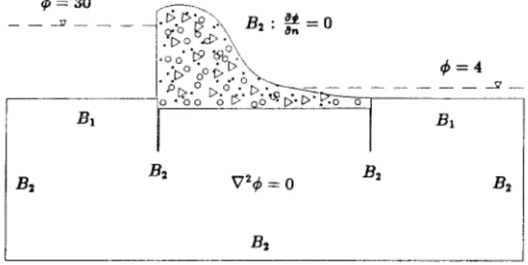
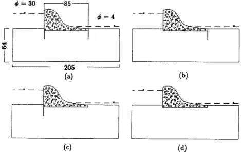
Sheet piles or cutoff walls oRen occur in problems of flow through porous media as shown in Fig. 1. Several actual civil engineering problems involving a wall have been noted, for example, a wall to retain a building excavation, a wall around a marine terminal, an anchored bulkhead for the ship dock, etc. [ 11. The dam and the sheet pile run for a considerable length in a direction perpendicular to the page and thus the flow underneath the sheet piles is two dimensional.

In studying potential scalar or vector problems, the analyst may encounter problems with singularity; nevertheless, the singular behavior is often ignored in numerical methods with the expectation that the error will be limited to the vicinity of the singularity. However, it is essential and inevitable for the employed formulation to be capable of describing the singular behavior when the singularity arises from a degenerate boundary, for example, in sheet pile design in seepage problems where the singularity dominates the force exerted on the sheet piles, and in the determination of the stress intensity factor of fracture mechanics for crack problems, where the strength of the singularity is the very value to be

* Corresponding author.

(3)

J. T. Chen et al. I Finite Elements in Anulysis unri Des@ 17 (1994) I 20

BZ B2 024 = 0 BZ B2

B2

Fig. 1. Classical problem of seepage flow with sheet piles under a dam.

sought. The degenerate boundary refers to a boundary, two portions of which approach each other such that the exterior region between the two portions becomes infinitely thin. In finite elements, to tackle degenerate boundary problems, special treatments such as the quarter-point rule have been used, or special singular or hybrid elements have been developed; e.g., MSCNASTRAN Version 66 provides the capabilities of singular CRAC3D and CRAC2D elements for crack problems, but for potential flow problems with singularity, no counterparts have been developed in the said commercial program to the authors’ knowledge.

In recent decades, the boundary element method has been evolving to be a widely accepted tool for the solution of engineering problems. The easy data preparation due to one dimension reduction makes it attractive for practical use. However, for problems with singularity arising from a degenerate boundary, it is well known that the coincidence of the boundaries gives rise to an ill-conditioned problem. The subdomain technique with artificial boundaries has been introduced to ensure a unique solution. The main drawback of the technique is that the deployment of artificial boundaries is arbitrary and, thus, cannot be implemented easily into an automatic procedure. In addition, model creation is more troublesome than in the single domain approach. To tackle such degenerate boundary problems, dual integral formulations have been proposed in, e.g., Refs. [2-61 for potential/seepage/Darcy flows around cutoff walls/sheet piles, Refs. [3,7,8,9, lo] for crack problems, Ref. [ 1 I] for thin airfoils in aerodynamics. Using the dual integral formulations, all the aforementioned boundary value problems can be made well-posed and solved effectively in the original single domain.

In this paper, the boundary element method based on the formulation of the dual integral equations proposed in [2-61 is employed, and the general purpose program boundary element potential 2-D (BEP02D) is developed to analyze the seepage flow under a dam with sheet piles. To facilitate computation of the seepage flow along and near the boundary, an expression for the flux tangential to the boundary is also derived and implemented in BEP02D. Several examples are furnished and the boundary element solutions using BEP02D are compared with analytical solutions if available and with the finite element solutions using MSCNASTRAN. The boundary effect and the design phase of the examples are also discussed in this paper.

2. Integral formulation of BEM

(4)

J.T. Chen et al. I Finite Elements in Analysis and Design 17 (1994) I-20 3

Governing equation:

02$(x) = 0, x in D, (1)

where V2 denotes the Laplacian operator, 4 is the potential head and D is the considered domain, bounded by the boundary B = B1 U Bl.

Boundary conditions:

$4~) = f(x), x on BI, (2)

W(x)

-

=

g(x),

an,

x on B2,

where f(x) and g(x) denote known boundary data, and n, is the unit outer normal at the point x on the boundary.

Using Green’s identity, the first equation of the dual boundary integral formulation for the domain point x can be expressed as follows:

27+(x) = s, ~(~,X)O(~) a(s) - J, Us d&s) (4)

for the two-dimensional case, while 27~ has to be replaced by 471 for the three-dimensional case. The following derivations will be devoted only to the two-dimensional case for simplicity. After taking the normal derivative of Eq. (4), the second equation of the dual boundary integral equations for the domain point x can be derived:

2n

Q(x)

-

=

SgM(S,X)$(S)

dB(s) -

lL(s,x)fp

dB(s).

an,

s

(5)

In Eqs. (4) and (5), U(s,x) := In(r), (6) (7)

(8)

(9) where r = 1s - xl, s and x being position vectors of the points s and x, respectively, and n, is the unit outer normal at point s on the boundary. Eqs. (4) and (5) together are termed the dual boundary integral formulation for the domain point. The explicit forms of the kernel functions are shown in Table 1. By tracing the domain point x to the boundary, the dual boundary integral equations for the boundary point x can be derived: a&x) = CPV s B T&x)&s) a(s) - RPV I B a(s,x)$$) d&s), s ay = HPV / M(s,x)+(s) M(s) - CPV/- L&x)? a(s), x B B s

(10)

(11)

(5)

4

Table 1

J. T. Chen et al. I Finite Elements in Anulysis and Design I7 (I 994) I -20

The explicit form of four kernel functions in dual integral equations

Kernel function .!J(s,s) T(.s,.r) L(.s..x) M(.s.s) Order of singularity Two-dimensional case Three-dimensional case Remark Weak In(r) -I,:r r’ = y,r; Strong mj.,n,‘r’ pj3!?l,:,-’ II, = n,(s) Strong >,,ti,!r’ >,,fi,/r’ fi, = n,(x) Hypersingular

7 I’ 1‘ n n lY4 _{1. I 1 I,} - n,ii,,r-- 3,~,j~,n,fi,:r’ n,ii, r’

I’, = .X, .s,

where RPV is the conventional Riemann or Lebesque integral, CPV is the Cauchy principal value, HPV is the Hadamard or Mangler principal value [ 12,131, and a = rr in the case of a smooth boundary. For a nonsmooth boundary, special care should be taken [20]. Eqs. (10) and ( 11) are called the dual boundary integral formulation for the boundary point. It must be noted that Eq. (1 1) can be derived just by applying the operator of normal derivative to Eq. (10). The commutativity property of the trace operator (a limiting process) and the normal derivative operator provides us with two alternative ways to calculate the Hadamard principal value analytically [7]. First, L’Hospital’s rule is employed in the limiting process. Second, the normal derivative of the Cauchy principal value should be taken carefully by using Leibnitz’ rule, and then the finite part can be obtained. The finite part has been termed the Hadamard principal value in fracture mechanics [7,9,10] or Mangler’s principal value in aerodynamics [ 111.

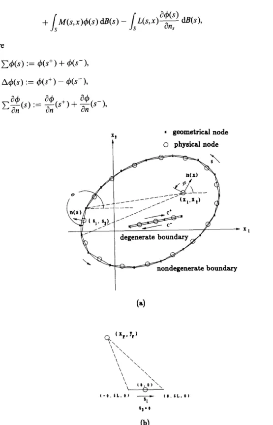
Consider a boundary B containing two parts, the nondegenerate boundary S and the degenerate boundary C+ + C- as shown in Fig. 2(a); i.e.

B=S+C++C-.

For x E S, Eqs. ( 10) and ( 11) can be rewritten as c+(x) = CPV

.I’ T(s,x)&s) d&s) - RPV I

G(s) U(s,x)--- a(s)

s dn,

+ i’ ‘kx)W) Ws) - .l:, c.(s.x).j$&) d&s),

.c \ (w(x) = HPV I M(s,x)#(s) d&s) - CPV G(s) c( an, . s . s I L(s,x)~ d&s)

+ / M(s,x)A&s) U(s) - k, L(r.i)Z+ d&s).

c. .s

For x E C+, the equations can be expressed as T(s,x)A~(s) B(s) - RPV (12) (13) (14)

Ws)

(15) aA

ad@)

p=HPV an, .I M(s,x)A&s) dB(s) - CPV c’ .I’ c ‘G,x)C

(6)

J. T. Chen et al. I Finite Elements in Analysis and Design 17 (1994) l-20 where C4W := 4@+ I+ 4Cs- >, W(s) := &+ I- 46- ), * geometrical node o physical node 7 nondegenerate boundary % (X,.7,) \ \ \ ’ \ ‘\\ \ _\ \ _\ \ _\ \ \ \ \ \ \ to. O)‘\\ A l-0. LL. 0) - 01 (0. LL. 0) Q-0 5

(16)

(17) (18) (19)

04

(7)

6 J. T. Chm et ul. I Finite Elements in Analysis and Design I7 (1994) I 20

A$(,) := $s+

) -

$s-

). ₍₂₀₎

Eqs. ( 17)-(20) reveal that the number of unknowns on the degenerate boundary doubles, and therefore the additional hypersingular integral equation ( 16) is, accordingly, necessary. The dual boundary integral equations for the boundary points provide complete constraints for the boundary data, rendering a well- posed boundary value problem. It must be noted that the compatible relations of the boundary data for x on Cf and those for x on C- are dependent; i.e., Eq. (15) for x on C’ and Eq. (15) for x on C are exactly the same equations, but Eq. (16) for x on C+ and Eq. ( 16) for x on C- are equations with different signs which are linearly dependent on each other. Nevertheless, we use Eq. ( 15 ) to model one side of the degenerate boundary and Eq. ( 16) to model the other side. Accordingly, Eq. ( 15) for .r on Cs and Eq. (16) for x on C- are linearly independent for the degenerate boundary unknowns. Hence. Eq. ( 16) plays an important role in the problem with a degenerate boundary. For the nondegeneratc boundary point, either Eq. (13) or (14) can be used.

3. Boundary element discretization and the closed-form integral formulae

After deriving the above compatible relationships of the boundary data as in Eqs. ( 13 t( 16), the boundary integral equations can be discretized by using constant elements as shown in Fig. 2(a), and the resulting algebraic system can be symbolized as

(21)

where [ ] denotes a square matrix, { } a column vector, and the elements of the square matrices are, respectively, U;i = RPV s U(S,,X~) a(Sj), (23) ?;, = -x&, + CPV J’ T(s,,x,)dB(s,), L;, = 71&j + CPV J L(S,,Xj) d&S,), (24) (25) M,, = HPV ./’ M(s,,x;) d&s,). (26)

All the above formulae can be integrated analytically. The closed forms of Eqs. (23)-(26) are summarized as follows:

First, we define the components of the unit outer normal vectors n(x) and n(s) as n,(s) = sin 0, IQ(s) = - cos 0,

n,(x) = sin 4, &(x) = - cos 4,

(27) (28)

(8)

J. T. Chen et al. I Finite Elements in Analysis and Design 17 (1994) I-20 7

which is shown in Fig. 2(a). The inner and cross products of the vectors are given by n(x)~n(s)=cos(~-~)=cosf$cos8+sin~sin8=31$i2+n’~‘,

n(s) x n(x)‘ek = sin(+- 6) = sin4cos@-cos4sin8 = -s’nz +&n’.

(29) (30) We use the following transformation:

x, { 1

=

Yr [- ::;E;] (::I::) ’

which is illustrated in Fig. 2(b). For the regular element, the integral formulae are

(31)

Uii = u lnJv2 + Y,’ - U + Yr tan-’ ( u/yr) I~2~~~f!x,,

Tij = tan-‘(U/Y,) I~~?~~?X,,

Lij = - COS(~ - @tan-‘(v/y,) - 0.5 sin(4 - 8)ln(n2 + y,‘) I~2~j&,

(32) (33) (34)

Mij = COS(4 -

e+---

u2 + y; - yr sin(+ - 0)

u2 : y2 ]U=O.SL-x, v=-0.X-x, 7

r (35)

where L is the length of the element. The integral formulae for the singular element are simply the limiting values of Eqs. (32)-(35); utilizing L’HBspital’s rule and the inverse triangular relations

tan-‘(x) + tan-‘( l/x) = ire,

X !Z tan-‘(x) = 1, (36) (37) we have Uij = L ln(0.5L) -L, (38) Tij = 0, (39) Lij = 0, ₍₄₀₎ A4ij = 4/L ₍₄₁₎

upon substituting x, = 0, y,. = 0, and 4 = 8. These closed-form formulae for constant elements indeed offer a clear explanation, which mainly comes from the joint behavior of sin (4 - 0) and cos (4 - 0) in Eqs. (34) and (35), of the general properties of the derivative of the single- and double-layer potentials as shown in Table 2.

4. Complementary solution tests and solution of domain and boundary data

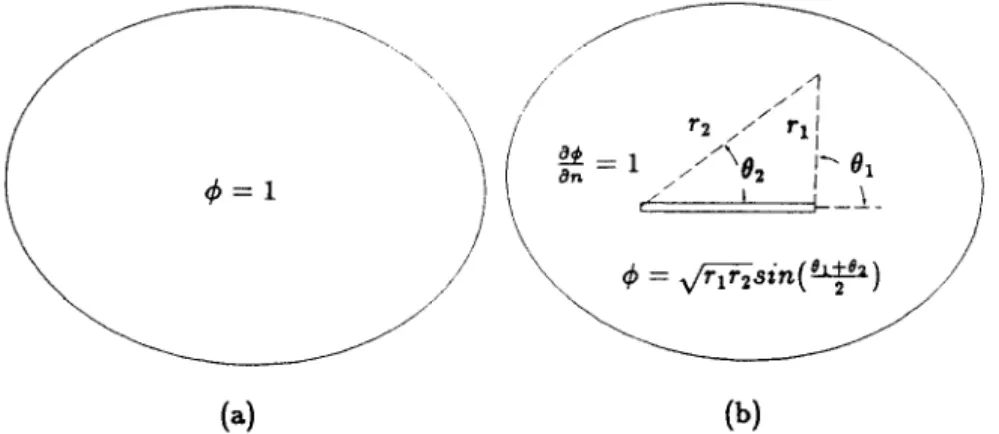
In order to test the above formulae, the complementary solution C$ = constant over the nondegenerate boundary as shown in Fig. 3(a) is tested for the matrices of [?‘ii] and [Mij]; thus, the singular diagonal term can be calculated from the minus sum of the off-diagonal terms in one row. However, for a degenerate boundary, this test for the diagonal terms fails, since the potential difference Ac$ vanishes on the degenerate boundary. To deal with this, two alternative techniques are available. In one, by

(9)

8 J. T. Chen et al. I Finite Elements in Anulysis and Design 17 (1994) 1 20

Table 2

The properties of single- and double-layer potentials

Kernel function U(s,x) 7-(&X) L(s.u) M(.s,.,-) L’(.s..u) M’(.S,.X) K(s,x)

Density function -?$!&I 4 +t,?t1 _(I, -h$/?t7 4

A.7 1

Potential type Single layer Double layer Normal deriva- Normal deriva- J K(s,x)&)ds

Tangent deriva- Tangent derivative of single- tive of double- tive of single- tive of double- layer potential layer potential layer potential layer potential Continuity across Continuous Discontinuous Discontinuous Pseudo-continuous Continuous Discontinuous boundary

Jump value No jump 2nd -2n&$/& No jump No jump ~~ ?nic$;in

introducing an artificial nondegenerate boundary which must be connected to the degenerate boundary under consideration to make a closed boundary enclosing a finite domain, and the problem is converted to calculating the regular terms on the introduced nondegenerate boundary [3]. In the other, we simply apply the complementary solution C#I = m sin(8r + f12/2) over the degenerate boundary as shown in Fig. 3(b), and the singular diagonal term can be calculated from the minus sum of the off-diagonal terms in one row.

Substituting the prescribed boundary conditions of Eqs. (2) and (3), we can reorder Eqs. (21) and (22), giving

where {u} is calculated by the known boundary data of the potential and normal flux. Then, solving Eq. (42) yields the unknown boundary data {x}. After-all the boundary unknowns are obtained, the fields of interior potential and flux can be calculated according to the boundary integral equations for the domain point as follows.

For x E D, the fields of 4(x) and a&~)/&~ can be written as

(10)

J. T. Chen et al. I Finite Elements in Analysis and Design 17 (1994) I-20

2na9(x)

_-

_{= /}

_M(s,x)A&s) _{U(s) -}

s,_

_L(s,x)+)

_d&s)

an,

c+

9

(43)

(44) If the flux along the boundary is to be considered, two methods are suggested to calculate it. One is the numerical derivative by using the boundary potential of Eq. (42), and the other is to describe an expression for it as will be elaborated upon later. Using the continuity and discontinuity properties of the tangential derivative of the single- and double-layer potentials as shown in Table 2 [ 141, the tangential flux along the boundary can be expressed as the superposition of all the boundary data of the potential 4 and normal flux 84/&r as in the following.

For x E S,

ado)

86(s)

’

at,

= HPV s M’(s,x)&s) u(s) - CPV I s L*(.s,x)~ d&s) + / $‘(s,x)A&) a(s) - s,+ L’(r,x)$$ u(s).

C+ (45)

For x E C+, a+(x) -=HPV

’ atx s C’ M’(s,x)A~(s) d&s) - CPV s C+

where tx is the tangential direction at the boundary point x and

L’(s,x) :=

“yx’,

x

M’(v) :=

a2u(s,x)

at an 9

x s

(47)

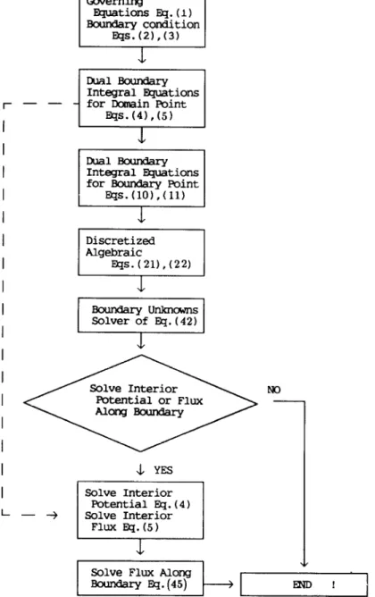
According to the above formulations, the general purpose BEP02D program of this mathematical model has been developed. The numerical implementation of the mathematical model is summarized in the flowchart of Fig. 4.

5. Finite element solution

In order to check the validity of the dual integral formulation, the finite element results are sought for comparison purposes. In industry, many commercial programs are available; e.g., MSCNASTRAN

(11)

IO J. T. Chen et ul. 1 Finite Elements in Anul.ysis und De.@n I7 (1994) I -20

I

hM1 Boundary Integral Elquations

r-- for Domain Point

,

i

I W.(4),(5) Dual Boundary Integral Quations 1 /

for Boundary Point EqS.(lO),(ll) I I I I I I I I I

I

I I I- Solve Interior Potential or Flux Alang Boundary & YES Potential EQ. (4) -+ Solve Interior

Fig. 4. Flowchart of the dual integral formulation BEM model.

provides the capabilities of structural analysis and heat conduction [15]. Using the analogy between steady-state heat conduction and the potential flow, the seepage problem can be simulated using the same Laplace model. In linear steady-state conduction, the time-dependent and nonlinear terms are ignored, leaving the following equation [ 151:

(12)

J. T. Chen et al. IFinite Elements in Analysis and Design 17 (1994) I-20 11

where u is the temperature field. There are two options, SOL 24 and 61 rigid formats in NASTRAN, to simulate the steady-state heat conduction problems. To the authors’ knowledge, the singular element of heat conduction has not been established yet; the quarter-point rule of CQUAD8 element is used in this paper. The output is the temperature and flux data. In the present finite element modelling, 485 GRID points, 420 CQUAD4, 10 CTRIA3 and 104 CELAS2 elements are used to simulate the four design cases (cases l-4) of Fig. 5 taken up in the following section. In order to discuss the singular behavior, the CQUAD8 element with the quarter-point rule of the last illustrative example (case 5) which has an analytical solution has been implemented. All the five examples have been solved by the BEP02D program and compared with the MSCiNASTRAN results and also with BEM supplemented by the subdomain technique (BEMl ).

6. Comparisons between FEM and BEM

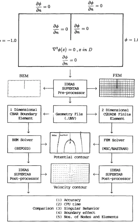
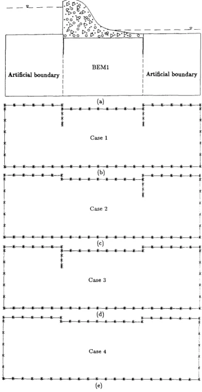
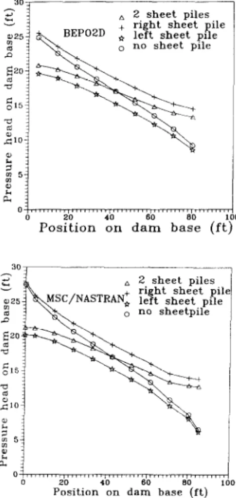
To simulate the seepage flow, the aforementioned FEM and BEM solvers were arranged as shown in the flowchart of Fig. 6 using the same pre-post processor. For the problem of Fig. 1, using the subdomain method(BEM 1) [ 161 and the BEP02D program, the results of the pressure head under the dam base match Lambe-Whiteman solution with a maximum error of 2% (see Fig. 7). It must be noted that the Lambe-Whiteman solution was obtained by free hand drawing [I]. There is no conclusion about which one is better because no exact solution is available. However, it can be said that the two BEM methods match very well with less than 1% difference. The BEMl method introduces an artificial boundary by using the subdomain technique as in Fig. 8 [ 161, whereas the BEP02D program is based on the dual integral formulation and only the true boundary needs to be discretized. In the design stages, the number and positions of sheet piles were investigated and optimized. Fig. 9 shows four design cases. The related meshes of BEM and FEM for four design cases are shown in Figs. 8 and 9. Fig. 10 shows the pressure

(4

Fig. 5. Four design cases of flow under a dam: (a) case 1, two sheet piles; (b) case 2, one right sheet pile; (c) case 3, one left sheet pile; (d) case 4, no sheet pile.

(13)

12 J. T Chen rt ul. I Finite Elements in Anulysis und Design I7 (I 994) 1 20 r$ = -1.0 I

?!L,

an

a4

0 -=

an

a4

-_=o

an

FL,

an

V2q5(z) =O,zinD a+ 0 an= 1 Dimensional cEmE8oundary q5 = 1.0 Velocity contour

(14)

J.T. Chen et al. IFinite Elements in Analysis and Design 17 (1994) I-20 13

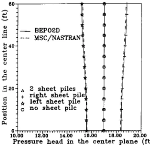
heads on the dam bases for different design cases. Fig. 11 shows the velocity in the x direction on the center plane under the dam. The boundary effect is present as usual and will be discussed in the following section. Fig. 12 shows the pressure head on the center plane under the dam. The difference in the velocities predicted by BEP02D and MSC/NASTRAN is larger while the predicted difference of the potential heads is smaller, as is usual. The comparison among BEP02D, BEMl and MSCNASTRAN is satisfactory. Based on the calculated turning moment for the four cases, case 3 is the stablest. After considering the safety of stability and seepage quantities, the best choice of design is suggested in Table 3.

The BEP02D program was executed on a VAX system and also on a CRAY X-MP system. The comparisons of MSC/NASTRAN and BEM in data preparation and CPU time are shown in Table 4. The easy data preparation and efficiency of the present model in case 5 with the analytical solution can be found under the same request of accuracy. Owing to the absence of the analytical solutions for cases 14, the CPU time is only for reference. For case 5, the analytical solution [ 171 is compared in Table 4 with the FEM and BEM solutions. The mathematical and numerical models are shown in Fig. 6. The pressure head and velocity contour of BEM and FEM are also presented in Fig. 6. After comparing the singular behavior with the analytical solution [ 171, it is found that FEM underestimates the velocity near the tip, but BEM overestimates as shown in Fig. 13. An explanation for the results is that the analytical I/,/? singular asymptotic behavior is approximated by a + br in the FEM model and l/r in the present dual integral BEM model. The results of subdomain analysis using linear elements for this problem oscillate seriously near the tip [ 171. Using the present formulation, even the constant element without singularity consideration can express the C” continuity properties of the flux along

FB+.

7. Discussions on boundary layer effect

It is known that the accuracy of the BEM solutions of the domain points near a boundary deteriorates rapidly as shown in Fig. 11, especially for the fluxes of the potential flow and the traction quantities of

lag

,,,,,,),,,,,,,,,,,,,,,,,,,,,,,,,,,, “,,I,,,_ P%tion400n claZ basea~ft) 1 Fig. 7. Flow under a dam.

(15)

14 J. T. Chen et d. I Finite Elements in Anulysis und Design 17 i 1994 / I 20

BEMI

Artificial boundary Artificial boundary

I I I I I I (4 ; *. *. *. _ r _ _ **a*****

1 I

_/

t

Case 1

T

I

t

: :

: .:.:::::::

::

: : :

(b) Case 2 : .~: : (4 : ._: ., *, ; *: ..: _ ~, T: *: : Case 4

Fig. 8. The related BEM meshes of four design cases: (a) BEM 1. two sheet piles with artificial boundaries(dotted line): (b) case 1, two sheet piles; (c) case 2, one right sheet pile; (d) case 3, one left sheet pile; (e) case 4. no sheet pile.

(16)

J. T. Chen et al. IFinite Elements in Analysis and Design 17 (1994) I-20 15

I i i i iiiiiiii

i4

Pi iiiiiii i i i i

(b)

(4

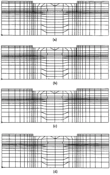
Fig. 9. The related FEM meshes of four design cases: (a) case 1, two sheet piles; (b) case 2, one right sheet pile; (c) case 3, one left sheet pile; (d) case 4, no sheet pile.

elasticity. The details of the behaviors depend on the numerical models used and are similar to those of the Gibbs phenomenon. This may be termed the boundary kz~~r e&t of the numerical model. To understand this phenomenon, the results of numerical experiments for the exact solution 4 = 0.5x are shown in Fig. 14, where it is seen that the domain of influence due to the boundary effect is about one characteristic boundary element length near the boundary. The region of influence provides the criterion of data selection for post-processing. MSC/NASTRAN can compensate for the boundary effect in Fig. 14. This example can explain why the boundary effect in Fig. 11 is present for BEM in comparison with the FEM results, which show no boundary layer effect. Using the criterion of data selection, the boundary effect can be smoothed if the boundary data are correct enough.

(17)

16 J. T. Chen et ul. I Finite Elements in Anulysis and Design I7 (I 994) I ~20

A 2 sheet piles

BEPO2D i left sheet pile right sheet pile no sheet pile

___~ -_.

2 sheet piles right sheet pile left sheet pile no sheetpile 1

0

PZsition400n da: baseso 1

i

0

Fig. IO. The pressure head on the dam base of different design cases

Velocity in x direction

(18)

J.T. Chen et al. IFinite Elements in Analysis and Design I7 (1994) I-20 17

Pressure head in the center plane

Fig. 12. The pressure head on the center plane under the dam.

b 2 -0.30

a A MSC/NASTRAN z o ANALYTICAL SOLUTION

12 -0.40 + BEPOZD (10 ELEMENTS on MEET PILE : t BEPOZD ( 5 EIJWENTS on SHEET PILE a

-0.50 ,,,,,!,,,,,,,,,,,,,,,,,,,,,,,,,,,,,,,,,,,,,,,,,,

0.00 2.00 4.00 8.00 8.00 1c

Velocity in x direction

Fig. 13. Velocity in the x direction along boundary FB’.

8. Conclusions

The dual integral formulation of a seepage flow through porous media has been presented here. Comparisons between the MSWNASTRAN and the BEM programs were discussed with respect to four design cases. It has been ensured that the capabilities of BEP02D in seepage flow analysis are acceptable after comparison with the analytical solution and MSC/NASTRAN results. It has been found that the BEM in the context of the present formulation is particularly suitable for the problem with singularity arising from a degenerate boundary. For a flow field with singularity in a homogeneous medium, BEM is superior to FEM not only in data preparation but also in accuracy and CPU time as shown in case 5 of Table 4. For engineering practices, since model creation requires the main effort, the present BEM, free from the development of an artificial boundary, is strongly recommended for industrial applications.

(19)

J. T. Chen et al. I Finite Elements in Analysis and Design 17 (1994) I 20 B X 4 BOUNDARY ELBMENTS 5 d E -x CD E Boundary effect

FLUX ALONG X DlFZCl'lON FOR X=0.6

3 X 4 BOUNDARY ELEMENTS + K * Boundary effect

1

FLUX ALONG X DIRECTION FOR X=0.5

NEUbUNN BOUNDARY CONDITION

,5

Governing equation II g

-8

V’C$ = o z in D

NEUMANN BOUNDARY CONDIllON

7 X4BOUNDARY ELEMEENTS

I ’ .q,’ ’

Boundary effect FLUX ALONG X DIRECTION FOR X=025

5 X4BOUNDARY ELEMENTS

FLUX ALONG X DIRECTION FOR X=0.5 10 X 10 FINITE ELEMBNTS

FLUX ALONG X DIRECTION FOR X=0.5

(20)

J. T. Chen et al. I Finite Elements in Analysis and Design 17 (1994) I-20 19

Table 3

The choice of optimum design

Case 1 Case 2 Case 3 Case 4

No. of sheet piles Seepage quantity Stability of dam 2 Best Fair l(right) Fair Fair l(left) Fair Best 0 Worst Worst Table 4

The comparisons of FEM and BEM

Case 1 Case 2 Case 3 Case 4 Case 5”

No. of sheet piles 2 l(right) l(left) 0 l(center)

No. of nodes (FEM) 485 479 479 473 871

No. of nodes (BEM) 72 64 64 56 40

No. of elements (FEM) 430 430 430 430 200

No. of elements (BEM) 72 64 64 56 40

CPU(min:sec) FEM on VAX785 02:20.29 02:17.51 02:17.61 02: 17.46 02:56.88 CPU(min:sec) BEM on VAX785 06: 10.87 04:52.07 04:53.75 03:43.73 01 z54.75

CPU(min:sec) BEM on CRAY 0.4530 0.3701 0.3699 0.2955 0.1697

a The comparison is fair under the same request of accuracy, since the analytical solution for this case is available.

Acknowledgements

The authors gratefully thank Prof. A.H.D. Cheng of the University of Delaware for providing the analytical solution used in Fig. 13.

References

[l] W.B. Lambe and R.V. Whiteman, Soil Mechanics, Wiley, New York, pp. 266-280, 1967.

[2] H.-K. Hong and J.T. Chen, Exact solution of potential flow around a line pump and on supersingularity of normal derivative of double layer potential, Proc. 10th National Conference on Theoretical and Applied Mechanics, pp. 571-574, 1986 (in Chinese).

[3] J.T. Chen and H.-K. Hong, Boundary Element Method, 2nd ed., New World Press, Taipei, Taiwan, 1992 (in Chinese). [4] J.T. Chen and H.-K. Hong, “On the dual integral representation of boundary value problem in Laplace equation”,

Boundary Elements - Abstracts and Newsletter 4 (3), pp. 114-l 16, 1993.

[5] J.T. Chen and H.-K. Hong, “Application of integral equations with superstrong singularity to steady state heat conduction”, Thermochimica Acta 135, pp. 133-138, 1988.

[6] J.T. Chen and H.-K. Hong, “Singularity in Darcy flow around a cutoff wall”, in Advances in Boundary Elements, VoL2, Field and Flow Solution, edited by CA. Brebbia and J.J. Conner, pp. 15-27, 1989.

[7] J.T. Chen, On Hadamard principal value and boundary integral formulation of fracture mechanics, Master Thesis, Supervised by Prof. H.-K. Hong, Institute of Applied Mechanics, Taiwan University, Taipei, Taiwan, 1986.

(21)

20 J. T. Chen et ul. I Finite Elements in Analysis und Design 17 (1994) I 20

[8] J.T. Chen and H.-K. Hong, “On Hadamard principal value and its application to crack problems through BEM”. Tllc~

11th National Conference on Theoretic-u1 und Applied Mechunics. pp. Q-837, Taiwan, 1987.

[9] H.-K. Hong and J.T. Chen, “Derivations of integral equations in elasticity”, Jownul cfEngineerin(g Mc7chunic.s DiGion. ASCE, EM5 114 (6), pp. 1028-1044, 1988.

[IO] H.-K. Hong and J.T. Chen, “Generality and special cases of dual integral equations of elasticity”. J. CSME 9 ( I ). pp. l-19, 1988.

[Ill C.S. Wang, S. Chu and J.T. Chen, “Boundary element method for predicting store airloads during its carriage and separation procedures”, in: Grilli et al. (eds.), Computational Engineering with Boundurj, Elements, Vol. 1. Fluid c177ti

Potential Problems, CMP Publ., pp. 305-3 Il. 1990.

[I21 J. Hadamard, Lectures on Cauchy’.s Problem in Lineur Purtiul Dlfirentiul Equutions. Dover Publications. Inc., Mineola, N.Y., 1952.

[ 131 K.W. Mangler, Improper integrals in theoretical aerodynamics, RAE Report 2424, I95 1,

[ 141 N.M. Giinter, Potential Theory and Its Applications to Basic Problems of’ Muthematical Phy.sic,.s. Frederick Ungar

Publishing, Co., N.Y., 1967.

[ 151 W.H. Booth (ed.), MSCINASTRAN Handbook for Thermal Analysis, The MacNeal Schwendler Corporation, 1986. [I61 O.V. Chang, Boundary elements applied to seepage problems in zoned anisotropic soils, MSc. Thesis, Southampton

University, 1979.

[ 171 O.E. Lafe, J.S. Montes, A.H.D. Cheng, J.A. Liggett and P.L-F. Liu, “Singularity in Darcy flow through porous media”.

J. Hydrutd. Dir. ASCE 106 HY6, pp. 977-997, 1980.

[ 181 J.T. Chen, S.L. Lin, W.R. Ham, C.Y. Chiou and W.T. Chin, MSCINASTRAN Primer und Engineering Applications..

Liang Yi Book Co., Taipei, Taiwan, 1989 (in Chinese).

[ 191 L.J. Gray, “Boundary element method for regions with thin internal cavities”, Engineering Anu1y.si.s with Boundury

Elements 6 (4), pp. 180-I 84, 1989.