SEEKER: An Adaptive and Scalable Location Service for Mobile Ad Hoc Networks

全文

(1)SEEKER: An Adaptive and Scalable Location Service for Mobile Ad Hoc Networks Jehn-Ruey Jiang and Wei-Jiun Ling Department of Computer Science and Information Engineering National Central University, Jhongli city, 320, Taiwan, R.O.C E-mail: [email protected], [email protected]. ABSTRACT Location-based routing protocols for mobile ad-hoc networks (MANETs) use geographic information to achieve higher scalability and lower control overhead than those of the topology-based routing protocols, e.g. AODV and DSR, etc. However, location-based routing protocols rely on location services to acquire the location information of the destination node so that they can forward packets to the destination properly. To keep the advantage of the location-based routing protocol, the location service should have high scalability and low control overhead. This paper proposes a location service called SEEKER to accomplish such goals. The basic idea of SEEKER is aggregate update, which integrates a group of position updates for the purpose of performing them altogether. In this way, a lot of location maintenance (update) overhead is reduced, while query success rate is still kept comparably high. Moreover, SEEKER can adapt to mobility by changing the frequency of location updates, which can further reduce the overhead. We simulate SEEKER and compare it with related location services. The results show that SEEKER has comparably good performances.. 1:. Introduction. The mobile ad hoc network (MANET) has attracted a lot of attention in recent years. A MANET consists of a collection of wireless mobile nodes that dynamically form a temporary network without the aid of pre-established infrastructure or centralized administration. A node in such a network acts as a host and a router; it sends data packets to other nodes and help forward packets for other nodes. Since the topology of a MANET changes frequently and unexpectedly, routing in it is a fundamental problem to be solved. Existing routing protocols for MANETs can be classified into two categories: topology-based and location-based ones. Topology-based protocols assume no knowledge of mobile node’s position. They can be further divided into proactive (for example, DSDV [20]), reactive (for example, DSR [21] and AODV [22]) and hybrid strategies (e.g., ZRP [23]). These protocols establish packet routes by flooding route requests to the entire network in an on-demand manner and/or by maintaining global (or zone-wide for hybrid protocols) node connection states constantly. As the network size or the number of nodes grows, such protocols’ performances degrade. dramatically due to the enormous increase of control packet overheads. Topology-based routing protocols thus have limited scalability [12]. On the other hand, location-based routing protocols, such as GPSR [19] and DREAM [18], etc., forward packets by utilizing nodes’ location information derived from positioning systems like GPS. Such protocols allow a node to forward data packets according to only the positions of itself and its neighbors. Location-based routing protocols are thus more scalable than topology-based ones. To route a data packet by a location-based routing protocol, there must be a location service for the source node to retrieve the location of the destination node. The location service must be scalable to preserve the scalability of the location-based routing protocols. Several location service protocols [4], [5], [6], [7], [8], [9], [10], [11], [12], [13], have been proposed. They can be classified into two categories: flooding-based and rendezvous-based. The former demands a (destination) node to broadcast its location to every other node proactively, or demands a (source) node to flood queries over the entire network for looking up the destination node’s location before sending data packets. On the other hand, the latter demands all nodes to agree upon a mapping that maps each node’s ID to one or more other nodes serving as location servers. These will be the rendezvous nodes where location updates and queries happen. Since the latter are more scalable than the former, in the following text we will focus on the latter only. Existing rendezvous-based location service protocols utilize the concepts of quorum-based (like XYLS protocol [4]), hierarchical-based (like GLS protocol [7]), and hash-based (like SLURP protocol [9]), and so on. This paper proposes a location service called SEEKER to achieve high scalability and low control overhead. The basic idea of SEEKER is aggregate update, which integrates a group of position updates for them to perform altogether. The network area is divided into square regions. A node’s position updates are aggregated and forwarded to the nodes of the regions in both the east and west directions. Some of the nodes receiving the updates will play the role of location servers of the node. And a node just sends location query to the nodes of the regions in the north and south directions. In this way, a lot of location maintenance (update) overhead is reduced, while query success rate is kept comparably high. Moreover, SEEKER can adapt to mobility by changing the frequency of location updates. This can make SEEKER save more location update overhead. We simulate SEEKER in terms. - 646 -.

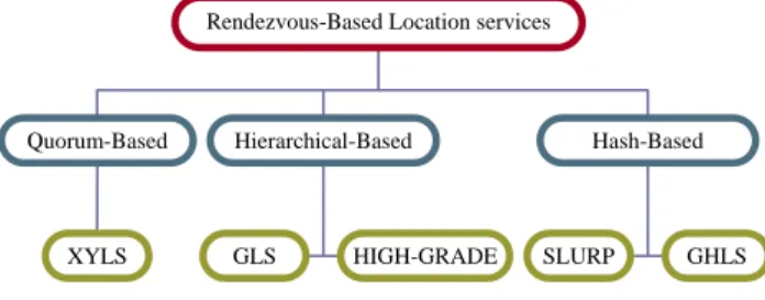
(2) of four metrics: the location maintenance cost, the location query cost, the query success rate, and the packet delivery rate for the comparison with two location services – GLS and HIGH-GRADE. The results show that SEEKER has comparably good performances. The rest of this paper is organized as follows. In section 2, we introduce some related work. In section 3, we present the proposed protocol, SEEKER. A performance comparison study is described in section 4 and concluding remarks are drawn in section 5.. 2:. Related work. In this section, we first introduce location-based forwarding in section 2.1. We then introduce rendezvous-based location services. There are a variety of such services, namely XYLS, GLS, HIGH-GRADE, SLURP, and GHLS, etc. Those protocols can be classified into the quorum-based, the hierarchical-based and the hash-based location services. Figure 1 shows the classification of those location services. We will describe the basic idea for each class of services. It is noted that in location-based routing and location services, each node is assumed to know the positions of itself and its neighbors. This can be achieved by equipping each node with a positioning device and by demanding every node to periodically send Hello packet (or beacon packet) containing its ID and position.. Figure 2: The “hole problem” of the greedy forwarding.. 2.2:. Quorum-Based Location Service. In a quorum-based location service, a node updates its position by sending the information to a subset (update quorum) of nodes. When a source node wants to transmit a packet to a destination node, it requests the location for the destination from a subset (query quorum) of nodes. The two subsets must be designed properly to have common nodes. Therefore, the up-to-date location information can be obtained for any given destination. Several quorum-based location services have been developed. For example, XYLS [4] is one of such services. In XYLS, when a node wants to update its current location, the node transmits the location information to an update quorum of nodes that are located along the north-south (column) direction (please see Figure 3).When a source node wants to transmit a packet to a destination node, it sends a query request for the location of the destination to a query quorum of nodes that are located along the east-west (row) direction.. Rendezvous-Based Location services. Quorum-Based. XYLS. Hierarchical-Based. GLS. HIGH-GRADE. Hash-Based. SLURP. GHLS. Figure 1: The classification of rendezvous-based location services.. 2.1:. Location-based forwarding. Assume that a source node intends to send packets to a destination node. If the position of the destination node is known, then the source node can make the packet forwarding decision on the basis of positions of its immediate one-hop neighbors and the destination node [14]. The greedy forwarding strategy is a simple way to forward a data packet. For example, in MFR (most forward within fixed transmission range) strategy [15], a node forwards data packet to its neighbor that is closest to the destination node. Such a strategy tries to minimize the number of hops a packet has to travel before reaching the destination node. Unfortunately, by the greedy forwarding strategy, a node may fail to forward a data packet when a local maximum is encountered. As shown in Figure 2, such a situation causes a void area and leads to the so-called Hole problem that prevents the data packet from reaching the destination even though there actually exists a path between the source node and the destination node. The face routing [16] and the perimeter routing [17] can be used to solve the problem.. Figure 3: Location update and query in XYLS.. 2.3:. Hierarchical-Based Location Service. For a hierarchical hash-based location service protocol, the area in which nodes reside is recursively divided into a hierarchy of grids (squares). For each node, one or more nodes in the grids at each level of the hierarchy are chosen as its location servers. Location updates and queries traverse up and down the hierarchy. There are several hierarchical rendezvous-based location services proposed in the literature. For example, Grid Location Service (GLS) [7] is one of such services. In GLS, the network area is arranged as a hierarchy of grids (squares) of different sizes. The smallest square is called an order-1 square. Four order-1 squares form an order-2 square, four order-2 squares form an order-3 square, and so on. A node chooses its location server for each square by selecting nodes in the square with the ID that is closest to and is circularly in advance of its own ID. Let’s take an example shown in Figure 4. Node 17 selects nodes 2, 23, 63 as its order-2 location servers; nodes 26, 31,. - 647 -.

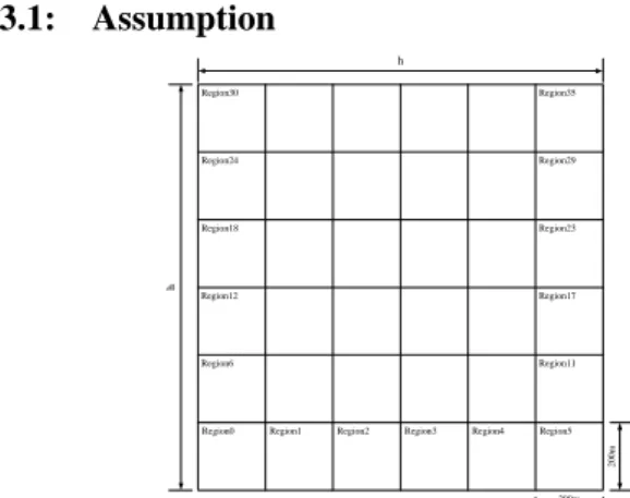
(3) and 43, order-3 location servers. When a source node wants to transmit a packet to a destination node, it sends a query request for “the best node” in order-1 square. The best node means the node with the ID that is closest to and is circularly in advance of the destination’s ID.. In this section, we describe the proposed location service – SEEKER. The basic idea of SEEKER is aggregate update. By aggregate update, the proposed service not only reduces a lot of protocol control overhead but also achieves a high accuracy in location query. Moreover, SEEKER can adapt to mobility by changing the frequency of location updates, which can further reduce the overhead. We present the implementation details of the service as follows.. 3.1:. Assumption h Region35. Region24. Region29. Region18. Region23. Region12. Region17. Region6. Region11. Query h. Update. Region30. Figure 4: Location update and query in GLS.. Hash-based Location Service (SLURP). The hash-based location service is also known as the home region location service. By the mapping of a hash function, each node is associated with a home region in such a service. A home region (also called a virtual region in [6] and [26], or called a home agent in [5]) of a node is either defined by a rectangular area or a circular area. One, some or all nodes in the area are supposed to be the location servers of the node. When the node wants to update its location, it sends the location information to its location servers in the home region by a location-based routing protocol. When a source wants to transmit a packet to a destination, it first figures out the home region by hashing destination node’s ID. It then sends query requests to location servers residing in the home region by a location-based routing protocol. There are many home region location service protocols proposed. For example, SLURP (Scalable Location Update-Based Routing Protocol) [9] is one of such services.. Figure 5: Location update and query in SLURP.. In SLURP, the whole geographical area is divided into equal-sized squares (see Figure 5). A node is associated with one of the squares by the hashing function that maps the node’s ID to the center of the associated square. The square is the home region of the node; all the nodes in the square are the location servers of the node.. 3:. The SEEKER Location Service. Region0. Region1. Region2. Region3. Region4. Region5 200m. 2.4:. 200m. Figure 6: The Area is divided into h × h square regions.. We assume that all nodes in the system are equipped with positioning hardware that provides them with their current locations. Each node is assumed to know the positions of itself and its neighbors, which is achieved by demanding every node to periodically send beacon packets containing its own ID and position. Also we assume that the whole network area is divided into h × h square regions. Figure 6 illustrates the network which is divided into 200m ×200m squares.. 3.2:. Location update. SEEKER allows few nodes to initiate location updates; those nodes are called initial nodes. Initial nodes must send location update packets (LOC for short) periodically. A node checks its neighbors in the east and west directions. If there is no node to the east of the node, it will be the initial node to send LOC to the west direction. On the other hand, if there is no node to the west of the node, it will be the initial node to send LOC to the east direction. If there are no neighbors in both east and west directions, it indicates that the node is isolated. For such a case, the node need not send any packets. The initial node sets a virtual destination to deliver the LOC packet to. The virtual destination has the y coordinate the same as the initial node’s y coordinate and has the x coordinate to the extreme in the west or east direction. The LOC packet is relayed by greedy forwarding until it reaches the terminal node, which is the westernmost (or easternmost) node closest to the west (or east) virtual destination. Every node periodically checks if itself is an initial node to deliver the LOC packet. Below, we describe the process of delivering the LOC packet. The initial node puts its own and all its neighbors’ IDs and location information in the LOC packet. It then delivers the LOC packet to the virtual destination by greedy forwarding. On the way from the initial node to the terminal node, every intermediate node gathers from the LOC packet new node IDs and location information. It stores the gathered information and. - 648 -.

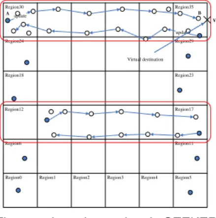
(4) append to the LOC packet its own and all its neighbors’ ID and location information. In this way, the nodes in the path from the initial node to the terminal node serve as the location servers for all the nodes in the same row of regions. We call the above process the aggregate update scheme. Region30 A update. Region35 B V update. Region24. Region29. Virtual destination Region18. Region23. Region12. Region17. Region6. Region11. Region0. Region1. Region2. Region3. Region4. the current node checks if there exists location information of destination node. If so, the current node sends a QREP packet containing the destination node’s location to the source node by using greedy forwarding. If not so, the current node must broadcast a B-QREQ packet and wait for a turn-around time to expect that any neighbor will reply. If one of its neighbors knows the destination’s position, it will broadcast a B-QREP packet to the current node. After receiving B-QREP packet, the current node sends a QREP packet to the source node by greedy forwarding. On the other hand, if the current node does not receive QREP packet after the turn-around time, it must deliver the QREQ packet to the next hop node in the north (or south) direction. The resending of QREQ terminate when the node nearest to the north or south extreme point is reached. Region30. Region5. Region35. Region29 B. Figure 7: Location update in SEEKER. Region23. Figure 7 illustrates an example of the location update. Node A in region 30 is an initial node because there is no node in the same row to the west of itself. Node A will start to send a LOC packet to the virtual destination V in the east. The LOC packet is forwarded until it reaches the terminal node B, which is the easternmost node closest to the virtual destination V in region35.. A. Region17. Region6. Region11 D. Region0. Region1. QREQ. 3.3:. Location query. When a source node wants to query where the destination is, it starts the query procedure. The procedure uses four types of packets: QREQ, QREP, B-QREQ and B-QREP. QREQ (Query request) is a unicast packet to query the location of the destination node, and QREP (Query reply) is also a unicast packet to reply the location of to the destination node. B-QREQ is a one-hop broadcast packet to query the destination’s location, and B-QREP is also a one-hop broadcast packet to reply to the destination’s location. If the source node does not know the location of the destination node, it broadcasts the B-QREQ packets to query the location of the destination node and waits for a turn-around time to expect that any neighbor will reply. If one of its neighbors knows the destination’s position, it will broadcast a B-QREP packet to the current node. In addition to replying to the B-QREQ packet, the B-QREP broadcast packet also has the function of prohibiting other source node’s neighbors from sending B-QREP packets. When the source node successfully receives the B-QREP message the query procedure stops. Otherwise, the source node sends a QREQ packet to two of its neighbors by greedy forwarding to the north and the south extreme points. The north (resp. south) extreme point has the x coordinate equal to the source node’s x coordinate and has the y coordinate to the extreme in the north (resp. south) direction. After sending the QREQ, the source node will wait for a specific timeout interval for the replying QREP packet. After the timeout interval expires, the source node will restart the query procedure if there is no QREP packet received. The node receiving the QREQ packet is called the current node. The behavior of the current node is similar to that of the source node. On receiving the QREQ packet,. Forward data. S. Region2. QREP. Region3. Region4. B-QREQ. Region5. B-QREP. Figure 8: Location query and reply in SEEKER. (The solid line represents the query request sending, and dotted line represents the query reply sending.). Figure 8 illustrates an example of the location query. First, the source node S sends B-QREQ to query where the destination is. If one of S’s neighbors knows destination location, it will send B-QREP to S. But if no S’s neighbor knows the location, S will forward two QREQ packets to one S’s neighbor to the north and one S’s neighbor to the south. When S forwards QREQ to the north and QREQ arrives node A, node A sends QREP to S by greedy forwarding and then drops the QREQ packet if node A knows destination’s location. Otherwise, node A sends B-QREQ to its neighbors. Note that after S gets destination’s location, it can forward data packets to the destination node D by greedy forwarding.. 3.4:. Adaptive Location Update. We observe that there is a tradeoff between the update interval and the moving speed. If we fix the update interval, then we will lose the query accuracy while the node speeds up. Thus, we would like the update interval to be adaptive to the moving speed. The basic concept is for the terminal node to calculate the average speed of nodes within the same row. We demand each node to embed its speed in the beacon packet which is sent periodically. For our location update procedure, we demand nodes to calculate the average speed of itself and all neighbors and then to accumulate the speed inside a “cumulate-speed” field in the LOC packet as the packet visits each node. In this way, the terminal node can figure out the average speed for all nodes in the same row. Afterwards, the terminal node can decide the new update interval according to the average speed.. - 649 -.

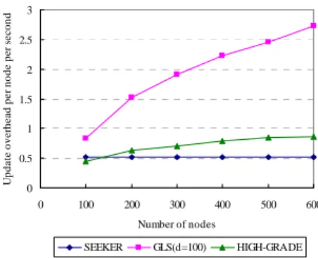
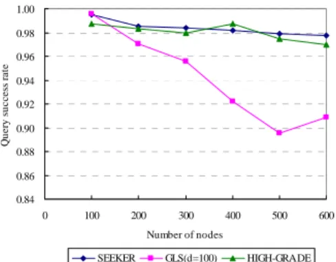
(5) retransmitted. Figure 9 shows the average location update cost as a function of the total number of nodes. The location update cost is measured by the number of location updates packets that are generated or forwarded per second. As shown in Figure 9, SEEKER has the smallest cost for almost all cases, and the cost grows very slowly with the increase of nodes. Figure 10 shows the average location query cost as a function of the total number of nodes. Location query cost is the number of query packets (QREQ and B-QREQ) that are generated or forwarded per second (note that the query reply packet is excluded). We can see the cost of SEEKER is lower than GLS and HIGH-GRADE. Update overhead per node per second. After obtaining the new update interval, the terminal node will broadcast the new update interval to its neighbors by beacon packets. When its neighbors receive the beacon packets, they will change their update interval to follow the new one. Only the terminal nodes can affect other node's update interval. In this way, the update interval of the nodes in the easternmost (or westernmost) regions will be changed. The update interval is also embedded in the LOC packet. The LOC packet is delivered by greedy forwarding. On receiving the LOC packet, the node changes its update interval according to that of the LOC packet. Moreover, the node will also broadcast the new update interval to all its neighbors. In this way, the update intervals of the nodes in the same row of regions will be changed. Below, we explain how to transform speed levels to update intervals. In Table 1, we define some speed levels with 1.25 m/s, 2.5 m/s, 5.0 m/s, 7.5 m/s, 10.0 m/s, and 12.5 m/s as the representative speeds. The update interval for a speed level is calculated as follows: Update interval = Transmission range / Representative speed. For example, if the average speed is 6 m/s, then the representative speed is 5.00 m/s and the update interval is 50 seconds (recall the transmission range is 250m)... 3 2.5 2 1.5 1 0.5 0 0. 100. 200. 300. 400. 500. 600. Number of nodes SEEKER. GLS(d=100). HIGH-GRADE. Table 1: The range of speed levels and their update intervals.. 4:. Representative Speed 1.25 m/s 2.50 m/s 5.00 m/s 7.50 m/s 10.00 m/s 12.50 m/s. Update Interval 200 (s) 100 (s) 50 (s) 30 (s) 25 (s) 20 (s). Figure 9: Update cost as a function of the number of nodes. 0.7 Query overhead per node per second. Range of Speed Levels 0 ~ 1.25 m/s 2.50 ± 1.25 m/s 5.00 ± 1.25 m/s 7.50 ± 1.25 m/s 10.00 ± 1.25 m/s 12.50 ± 1.25 m/s. Simulation Results. 0.6 0.5 0.4 0.3 0.2 0.1 0 0. 100. 200. 300. 400. 500. 600. Number of nodes. We simulate SEEKER by ns-2 [24]. IEEE 802.11 [1] is used as the basis of wireless communication. The maximum number of nodes is assumed to be 600 and each node is assumed to have 2 Mbps communication bandwidth with 250m transmission range. The nodes are assumed to be placed at uniformly random position in the square area. The node density is kept about 100 nodes / km2. For example, for the case of 600 nodes, the square area is 2400 m × 2400 m. We adopt random waypoint [2] as the mobility model. Every node is assumed to have a random destination and a random speed between 0 m/s and 10 m/s. Each time the node reaches the destination, it chooses a new destination and begins to move toward it immediately (i.e., there is no pausing time). We choose a beacon (hello packet) period of 2 seconds. Several performance metrics are evaluated to compare SEEKER with GLS [7] and HIGH-GRADE [10]. Each data point is the average of 5 experiment results and each experiment runs for 300 seconds. Each node periodically broadcasts it location information to its neighbors by using HELLO packets that generated every 2 seconds. Also each node generates on average 15 location queries for random destination nodes during the simulation. For example, in the case of 600 nodes, there will be totally 9000 queries. Like those in GLS and HIGH-GRADE, queries are not. SEEKER. GLS(d=100). HIGH-GRADE. Figure 10: Query cost as a function of the number of nodes.. Figure 11 shows the query success rate as a function of the total number of nodes. Similar to the GLS, queries are not retransmitted, so success means that each query request succeeds on the first try. We can see that SEEKER outperforms GLS and HIGH-GRADE in terms of query success rate. Below, we show the simulation results under the environment of data traffic which is of constant bit rate (CBR) and is generated by half of the nodes. Each connection lasts 20 seconds and has four 128-byte data packet per second. For example, for the case of 600 nodes, the total connections are 300, and each connection has 80 packets to send. Connections are initiated randomly between 30 and 280 seconds. Figure 12 shows the packet delivery rate (PDR) as a function of the total number of node. We can see that SEEKER is better than GLS. (Because HIGH-GRADE does not provide data for PDR, we do not compare SEEKER with it.). - 650 -.

(6) 1.00 0.98 Query success rate. 0.96. [7]. 0.94 0.92 0.90 0.88. [8]. 0.86 0.84 0. 100. 200. 300. 400. 500. 600. Number of nodes SEEKER. GLS(d=100). HIGH-GRADE. [9]. Figure 11: Query success rate as a function of the number of nodes.. [10]. 1.00. [11]. Packet delivery rate. 0.95 0.90 0.85. [12] 0.80 0.75. [13]. 0.70 0. 100. 200. 300. 400. 500. 600. Number of nodes SEEKER. [14]. GLS. Figure 12: The packet delivery rate as a function of the number of nodes.. 5:. [15]. Conclusion. [16]. In this paper, we propose a scalable location service called SEEKER for location-based routing in mobile ad hoc networks. SEEKER uses the concept of aggregate update to reduce the location management overhead and to keep high query success rate. Moreover, SEEKER uses the concept of adaptive update to adjust location update interval according to the level of the moving speed to further reduce the overhead without sacrificing query success rate. We simulate SEEKER and compare it with related location services. The simulation results show that SEEKER has comparably good performances in terms of scalability, maintenance cost and query success rate.. [17]. [18]. [19]. [20]. References [1] [2]. [3]. [4]. [5]. [6]. IEEE, “Wireless LAN medium access control (MAC) and physical layer (PHY) Spec,” IEEE 802.11 standard, 1998. Josh Broch, David A. Maltz, David B. Johnson, Yih-Chun Hu, and Jorjeta Jetcheva, “A performance comparison of multi-hop wireless ad hoc network routing protocols,”in Proc. ACM/IEEE MobiCom, pages85–97, October 1998. Barry M. Leiner, Robert J. Ruth, and Ambatipudi R. Sastry, “Goals and challenges of the DARPA GloMo program,” IEEE Personal Communications,3(6):34–43, December 1996. I. Stojmenovic, “A scalable quorum based location update scheme for routing in ad hoc wireless networks,” Technical Report TR-99-09, SITE, University of Ottawa, Sep. 1999. I. Stojmenovic, “Home agent based location update and destination search schemes in ad hoc wireless networks,” Technical Report TR-99-10, SITE, University of Ottawa, Sep. 1999. P.-H. Hsiao, “Geographical Region Summary Service for. [21]. [22] [23]. [24] [25]. [26]. - 651 -. Geographical Routing,” The ACM Symposium on Mobile ad hoc Networking & Computing (MobiHoc 2001) Poster Paper, Vol. 5, No. 4, Oct. 2001. J. Li, J. Jannotti, Douglas S. J. De Couto, D. R. Karger and R. Morris, “A scalable location service for geographic ad hoc routing,” Proceedings of the sixth annual international conference on Mobile computing and networking, Aug. 2000. Christine T. Cheng, H. L. Lemberg, Sumesh J. Philip, E. van den Berg, and T. Zhang, ”SLALoM: A scalable location management scheme for large mobile ad-hoc networks,” in Proceedings of IEEE WCNC, March 2002. S.-C. M. Woo and S. Singh, “Scalable routing protocol for ad hoc networks,” Wireless Networks, Vol. 7, No. 5, Sep. 2001. Y Yu, GH Lu, ZL Zhang. “Enhancing location service scalability with HIGH-GRADE,”in Proceedings of IEEE Mobile Ad-hoc and Sensor Systems, Oct. 2004. Y. Xue, B. Li, and K. Nahrstedt, “A scalable location management scheme in mobile ad-hoc networks,” in Proceedings of 26th Annual IEEE Conference on Local Computer Networks, pp. 102 -111, 2001. S. Das, H. Pucha, and Y. Hu, “Performance comparison of scalable location services for geographic ad hoc routing, IEEE INFOCOM, 2005. B. Seet; Y. Pan; W. Hsu; C. Lau, “Multi-home region location service for wireless ad hoc networks: an adaptive demand-driven approach,”WONS’05, Jan. 2005. M. Mauve, J. Widmer, H. Hartenstein, “A survey on position-based routing in mobile ad-hoc networks,” IEEE Network Magazine, 15(6):30 - 39, November 2001. H. Takagi and L. Kleinrock, “Optimal Transmission Ranges for Randomly Distributed Packet Radio Terminals,” IEEE Trans. Commun., vol. 32, no. 3, Mar. 1984, pp. 246–57. P. Bose et al., “Routing with Guaranteed Delivery in Ad Hoc Wireless Networks,”Proc. 3rd ACM Int’l. Wksp. Discrete Algorithms and Methods for Mobile Comp. and Commun., 1999, pp. 48–55. B. Karp and H. T. Kung, “Greedy Perimeter Stateless Routing for Wireless Networks,” in Proc. 6th Annual ACM/IEEE Int’l. Conf. Mobile Comp. Net., Boston, MA, Aug. 2000, pp. 243–54. S. Basagni, I. Chlamtac, V. R. Syrotiuk, and B. A. Woodward, “A distance routing effect algorithm for mobility (DREAM),” in Proceedings of ACM MobiCom 98, pages 76–84, 1998. B. Karp and H. Kung, “GPSR: greedy perimeter stateless routing for wireless networks,” in Proc. of the sixth annual international conference on Mobile computing and networking, pp. 243-254, 2000. C. E. Perkins and P. Bhagwat, “Highly dynamic destination-sequenced distance-vector routing (DSDV) for mobile computers,” in Proc. of ACM SIGCOMM, August 1994. D. B. Johnson and D. A. Maltz, “Dynamic source routing in ad hoc wireless networks,” Mobile Computing, Kluwer Academic, 1996. C. E. Perkins and E. M. Royer, “Ad hoc on-demand distance vector routing,” in Proc. of IEEE WMCSA, February 1999. Z. J. Haas and M. R. Pearlman, “The performance of query control schemes for the zone routing protocol,” in Proc. of ACM SIGCOMM, August 1998. The Network Simulator ns-2, http://www.isi.edu/nsnam/ns/. S. Ratnasamy, B. Karp, L. Yin, F. Yu, D. Estrin, R. Govindan, and S. Shenker, “GHT: A geographic hash table for data-centric storage in sensor nets,”in Proceedings of ACM WSNA, 2002. S. Giordano and M. Hamdi, “Mobility management: The virtual home region,” Technical Report SSC/1999/037, Ecole Polytechnique Federale de Lausanne, October 1999..

(7)