Internet Topological Properties Analysis and Performance Improvement

全文

(1)Internet Topological Properties Analysis and Performance Improvement Neng-Pin Lu and Shu-Chun Lin Department of Information Management Chang Gung University, Kwei-Shan, Tao-Yuan, Taiwan, 333, R.O.C [email protected], [email protected] set of links. Passing messages between any two nodes needs to route through a series of nodes and links. As the quantities of nodes and links increase, the routing cost would increase relatively. For the efficiency of network routing, the path length between any node-pairs should be as short as the network constructor can.. Abstract This paper is to analyze the Internet topology. The goal is to collect statistical data of the Internet structure and to compare the results with related theories, such as small-world networks and scale-free networks. In this paper, we sampled from network management, political, and economic aspects. In the three sets of samples, there are 191 web sites of Network Information Centers (NIC), 227 government portal sites, and 2004 Fortune Global 500 corporations’ web sites. To make sure the validities of the three sample set, an extra set of 10 thousand randomly sampled IP addresses were traced. The IP routing information from Chang Gung University to the sampled IP addresses was collected by traceroute-based utility: tracert and was stored into the database: eLinkage. Through statistical analysis of topological properties, small-world property and scale-free property were verified. Furthermore, we implemented our filtering algorithm, Kf, to figure out the rough backbone of the Internet. Finally, we designed two algorithms, Longest-path-first (LPF) and Random-link-added (RLA) methods to suggest improving the performance of the Internet.. On the other hand, a social network also can be represented by nodes and links which correspond to individuals and friendships. A social network is always tremendously large; however, the degrees of separation between any two people in social networks are amazingly small, around 6, as discovery by Milgram [18] and further modeling by Watts and Strogatz [24]. They called this phenomenon small-world effect which says that although there may be millions of individuals in the social network, yet everyone can reach any other person within a very short distance of connections. If the Internet has also the small-world effect, then any two computers can communicate with each other in shorter distance and higher bandwidth. Based on the research of W-S model [24], Albert et al. [2] found the web links exhibit in skewed degree distribution. They noticed that nodes had a non-uniform probability of being connected to others, with some nodes having extremely large numbers of neighbors (the so-called hub nodes). They called it rich-get-richer phenomenon. Such high variability of node degrees follows power law. Besides, there has been much research devoted to Internet topology [9, 12, 16, 21, 26]. . Keywords: topology analysis, scale-free networks, small-world networks, Internet. In this paper, we proposed a standard process to help researchers to observe the Internet topology. According to the process, we investigated the properties of small-world networks and scale-free networks of the Internet and design the backbone filtering algorithm to figure out the core component of the Internet. Finally, we conducted simulations with our algorithms to suggest the improving ways for the Internet.. 1. Introduction Internet, connecting all the computers around the world, has been indispensable in our daily lives and will influence our future societies enormously. The current Internet has been distributed growth so rapidly without controlled by a central authority. As a result, understanding the connected relationships between the core components of the Internet becomes more and more important. A lot of ongoing researches about improving the qualities of Internet service have been developing continuously.. 2. Related Work 2.1 Internet Structure. From the perspective of graph theory, we can abstract Internet as a graph with a set of nodes and a. Internet can be decomposed into several 1.

(2) thousand administrative subnetworks, as shown in Figure 1 [12]. These subnetworks are so-called domains. All hosts, routers, and links in a domain are administered by a single authority, and are addressed by IP addresses.. k=. n. k =. i =1 i. 2e n. (1). 0 ≤ e ≤ n ( n − 1) / 2 Path length: the number of links of the shortest path between any two nodes. The distance between two nodes i and j is defined as the number of nodes traversed by the shortest path connecting i and j. The minimum connected path between any two nodes of a graph is defined as d(i, j). The average shortest path length, l , that is the average value of shortest path length over all pairs of nodes can be denoted as. Figure 1 Internet structure [12]. l=. The Internet itself is a network of heterogeneous inter-connected networks, so network topology is a representation of the interconnection between directly connected peers in a network. Peers are ports on devices connected by a physical transmission link in a physical network topology and network layer processes need to consider the current network topology to be able to route packets to their final destination reliably and efficiently [19, 21]. In this paper, we consider the Internet topology as the logical IP topology, ignoring hubs and bridges and link-level details.. lPl (l ) ≡ l. 1 n(n − 1). n. n. d (i, j ). (2). i =1 j =1. Clustering coefficient: the value, ci, is the measure of the interconnectivity in the node’s neighborhood. “Clustering” refers to the tendency of forming cliques in the neighborhood of any given node in a network. In other words, if a node a is connected to b and at the same time, b is connected to c, then the probability of a connected to c is very high. Hence, we use ci to measure the average probability that two neighbors of the node i are also connected between them. Let us consider a node i with ki neighbors and denote ei, that is the number of the links between ki neighbors that actually exist. So that the average value of over all nodes with degree larger than one is defined as. 2.2 Graph Terminology and Notation The Internet topology we considered can be represented by a graph. All graphs considered in this research are finite, undirected and simple (i.e., without loops and multiple edges). A graph is a collection of vertices, pairs of which joined by edges [20]. Formally, a graph G = (V, E) is an ordered pair of finite sets V and E. The elements of V are called vertices (also known as nodes) and the elements of E are called edges (also known as links). Here, we abstract Internet as a graph with a set of nodes and a set of links and refer to above definitions. The nodes set contains computers or networking devices, including hubs, switches, routers, and so on. The links set is composed of connection exists between any two nodes.. c=. 1 n. n i =1. 2ei k i (k i − 1). (3). 2.3 Classical Graph Models In graph theory, there are two classical graph models: regular graph and random graph [10, 11]. A regular graph is a graph with n nodes, and each one connects with k closely neighbor nodes (See Figure 2(a)). Random graph, introduced by Erdös and Rényi [11], the so-called “Erdös-Rényi (ER) random graph model”, is on the opposite end of the graph spectrum. The connections between any two nodes are determined in a random way as shown in Figure 2(c). The regular graph with n nodes has n(n − 1)/2 links, while most large-scale real networks appear to be sparse, that is, most real networks are not fully connected and their number of links is generally of order n rather than n2.. Furthermore, some important properties of graph are described as below: Neighbor node: if the distance of a graph of i and j equals to 1, that means nodes i and j are the nearest neighbors. Degree: the degree ki of node i is defined as the number of links incident on node i of an undirected graph. Let n =. 1 n. V and e = E. exist. In contrast, an ER random graph with n nodes and about pn(n − 1)/2 links. So that ER random graph has a very small number of links. The main. 2.

(3) observation that highly popular nodes are more likely to be connected again in the process of incremental growth, the so-called “rich-get-richer” phenomenon [4, 10, 26].. goal of the random graph theory is to determine at what connection probability p a particular property of a graph will most likely arise. There has been a lot of researches are based on the Erdös-Rényi random graph model, in general, random graph can be used to model general networks.. Re-wiring: Remove some links randomly and rewire them according to the preferential connectivity mechanism.. 2.4 Small-world Networks. In such networks, nodes have a non-uniform probability of being connected to others, with some nodes having extremely large numbers of neighbors. This property presents in paper citation databases [23], actor collaboration networks [24], web links [2]. The nodes of a scale-free network are not randomly connected. Scale-free networks include many connected nodes, hubs of connectivity that shape and dominate the way the network operates. The ratio of heavy connected nodes to the number of nodes in the rest of the network remains constant as the network changes in size.. Small-world behavior, popularly known as six degrees of separation was mathematically formalized by Watts and Strogatz [24]. The small world concept was formally introduced by Stanley Milgram [18], a social psychologist professor at Harvard University, USA. He conducted an interesting experiment for the question that how many acquaintances would it take to connect two randomly selected individuals. In his experiment, there was 42 letters delivered correctly to the target person and the median number of people required to get the letters to the target was 5.5. Rounding it up to 6, Professor Milgram amazingly discovered the "six degrees of separation," under the condition that the separation was defined as how many contacts needed to connect two unfamiliar persons. Such phenomenon is called small-world effect.. Based on the pervious researches, we proposed a process to observe the topological properties: small-world properties and scale-free properties discussed above by analyzing of the shortest path length, the clustering coefficient, and the node degree distribution. Finally, we also suggested the plausible Internet performance improvement from the viewpoint of the topological properties.. Small-world graphs, as shown in Figure 2 (b), exhibit connectivity properties that are between random and regular graphs. Like regular graphs, they are highly clustered; yet like random graphs, they have typically short distances between arbitrary pairs of nodes. It has been shown that many networks have similar small-world property [2, 8, 12, 25].. 3. Methodology Figure 3 is our research flow for Internet topology analysis and the major steps are detailed in the following, respectively.. Figure 2 regular, small-world, and random graphs 2.5 Scale-free Networks Scale-free networks are particularly emphasized by the work of Barabási and Albert [1, 2, 5] who explored a promising class of models that yield strict power-law node degree distributions. In the so-called Barabási-Albert (BA) model, three generic mechanisms are defined as follows:. Figure 3 Research flow 3.1 Selecting Experimental Samples. Incremental growth: it follows from the observation that networks develop by adding new nodes or new connections.. We sampled from network management, political and economic aspects, which are 191 web. Preferential connectivity: it relies on an 3.

(4) Table 1 Definition of the chi-square goodness-of-fit test statistic. sites of NIC (Network Information Center) [29] around the world, 208 government portal sites, and 2004 Fortune Global 500 corporations [27]. To make sure the validities of samples, we use extra 10 thousand randomly sampled IP addresses.. Ho: The data follow the specified distribution Hypothesis: H1: The data do not follow the specified distribution. 3.2 Probing the Internet. Test statistic: χ o2 =. In this research, we used tracert1 utility to record all the networking devices where packets passing through from source node to the destination node [6]. With tracert to collect and record the routing path information between the sample websites or IP addresses, the kernel of this program is a for loop. The loop calls the DOS command shell to execute tracert for n iteration, where n is the number of all the sample websites or IP addresses.. (Oi − E i ) 2 Ei. k i =1. Oi : observed counts for bin i Ei : corresponding expected counts for bin i k : the number of classes. Significant level: Critical region: if χ o2 > χ (21−α ,. χ (21−α ,. k −c ). , reject Ho; otherwise, accept Ho. k −c ). Table 2 Graphical metrics. 3.3 Building “eLinkage” Database. Metric. After completion of routing data collection, we built a database called “eLinkage” for post-processing and further analyzing. The major purposes of the database include storage, calculation, integration, and analysis of routing data. The database will be helpful for the follow-up research.. Equation. a. Average degree. b. Average path l = length. k=. kP ( k ) ≡ k. lPl (l ) ≡ l. 1 n. n i =1. ki , ki =. 1 n( n − 1). n. n. i =1 j =1. n j =1. Aij. d ij. 2ei 1 n Clustering , e = 1 Aij A jl Ali c= i * 2 jl n i =1 k i (k i − 1) coefficient n: the number of nodes. Aij: Aij = 1 if node i and j is connected; otherwise, Aij = 0. ki: the number of links incident on node i. dij: the minimum value of connected path length between any two nodes. ei: the number of links among the neighbors of i which be computed in the adjacency matrix. * Since ci is undefined when ki = 1, this averaging used to calculate excludes nodes with only one neighbor. If a graph has many nodes with degree one, then all of them are ignored. For k i ≤ 1 we define ci. c. 3.4 Making Statistical Analysis In order to verify the reliability of our data, we compared the samples with the population [28] on the same date2 by nonparametric statistical method: chi-square goodness-of-fit test (See Table 1). Then, we obtained the estimator to support this research by some metrics, the node degree, the degree distribution, the shortest path length, and the clustering coefficient. The average degree in this research is defined as the average value of ki over all the nodes in the network, since each link contributes to the degree of a node. These metrics provide a basic and robust characterization of Internet topology [10, 13, 19, 20]. The equations are listed as shown in Table 2.. = 0 [19].. 3.5 Mapping Internet Topology We simplified layout of the Internet topology by the visualization tool and showed the map of the Internet.. 3.6 Doing Simulations. 1 2. Based on the statistical results, we tried to suggest improving performance of the Internet. Upon sampling the Internet topology, we conducted simulations with network models. In this paper, we conduct two simulation methods which can reduce the path lengths in Section 5. The essence of simulation is that using randomly links and decreased the longest path to create the key connections or downsize the number of large path length. Our experiment will suggest the. A traceroute utility on Microsoft Windows operation system. The data we collected all on the same time period of March, 2005. 4.

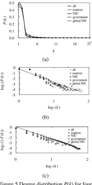
(5) performance improvement for the Internet.. IT NL FR. IT NL FR DE. 3.7 Making Discussion and Conclusion. DE CA KR. CA US. KR. Finally, we discussed the plausible proposal to improve the performance of the Internet based on our simulation results.. CN. US. UK. CN UK. JP. JP. (c). (b). Figure 4 Percentages of IP addresses applied to each region. 4. Analytical Results 4.1 Samples Testing. 4.2 Results of Metrics. In this research, we collected several routing data of the Internet by our method. To ensure the reliability of our sampled IP addresses, we compared the samples with the population. The data we collected all on the same time period of March, 2005. The hypothesis is if our samples came from a population with the hypothesized distribution. With the sampled random data, the number of k was 152. To make the chi-square approximation valid, the expected count should be at least 5. So we combined some bins in the tails of those counts are less than 5, and thus we got 90 bins. The Pearson' s. We quantified the size of each sample by counting the total number of nodes n and links e. Then the degree, the shortest path length, and the clustering coefficient could be computed. Notice that all of our defined metrics focus on the local view of Internet. In order to obtain the global view of Internet, counting the global behavior of these statistical measures is important. Thus, the statistical average value of each metric over all nodes is calculated. Table 3 reports the average values and gives some indications of the Internet topology.. chi-square statistic were computed: χ o = 107.1148 2 is smaller than χ (1−α , k − c ) = 112.022 , so we don’t reject the Ho hypothesis. The testing result shows that our sampled data are not different with the population of the applied IP addresses under 95% significant level. That is the distribution of sampled data is consistent with the population. The percentage of 90 bins (regions) is shown in Figure 4.3 Figure 4(a), is the comparison of the population and sampled data. Figures 4(b), 4(c) are the population and simple data presented individually by pie chart (labels are shown for the top 10 ranks only by space limitation). 2. Degree, k The degree of a node in Internet has an immediate interpretation, explaining how well a node is connected. The average degree is small because hosts (nodes) in general support a limited number of connections (interfaces). The average degree of our sampled data is from 2.24 to 2.67 as Table 3 shows, the value is quite quiet small if compared with network size and number of links.. Table 3 Average metrics of data Number of IP addresses(%). 0.6. Data. Population Sample 0.4. e. k. c. l. Random. 8,795. 9,916. 2.67. 0.0269 15.21. NIC. 1,096. 1,089. 2.24. 0.0449 13.75. Government. 1,189. 1,187. 2.28. 0.0332 14.21. Global 500. 1,935. 2,009. 2.40. 0.0294 14.07. All. 11,527. 12,691. 2.66. 0.0282 15.13. 0.2. 0.0. regions. (a). 3. n. Figure 5 reports the probability P(k) that any given node in our data has degree k. Figure 5(a) is the normal axis and it obviously follows the so-called power-law distribution; the most nodes have the same number of links (top left), only 1 or 2 links, and a few major hubs hold many times links. The ranking of Taiwan is 13th and percentage is 0.8%. 5.

(6) (bottom right). The curves of different samples all fit power law well. Both Figures 5(b) and 5(c) are degree distributions in the double logarithmic scale of P(k). Figure 5(b) is probability density functions (PDF) and complementary cumulative distribution functions (CCDF) is in Figure 5(c). The solid line are the power law decay k- with = 2.34.. The degree distribution on the double logarithmic scale appears approximately the linear behavior (See Figure 5(b)). This is a strong evidence to indicate it is very different from the bell-shaped of Poisson distribution. The distribution can be fitted by the power-law form. The degree distribution P(k) clearly show a high variability and the degree vary over a range close to two orders of magnitude. Many nodes in the graph have just a few connections, while a few hubs connect 10-fold or more links. More specific, the probability of only connected one or two links reaches to 86.05%. On the contrary, the maximum value of all data is 62 and the probability of those bigger than 50 is less than 0.01%. In prior study of Faloutsos et. Al [12] has pointed out that the connectivity properties of Internet are characterized by heavy tailed probability distributions that can be reasonably approximated by power-law forms. Our results also confirm their findings. 0.5. 0.3 0.2. F (k ) =. 1. 6. 11. Data. 21. (a) log10 (P (k )). all random NIC government global 500. (5). c. Random. -0.0394. 2.3246. Nic. -0.3705. 2.6147. Government. -0.2903. 2.72. Global 500. -0.2428. 2.4057. All. -0.0192. 2.3398. Path Lengths, l 0. 1. Despite the small node degrees discussed in pervious section, the shortest path length of nodes, l, is also small relatively. The shortest path length represents the minimum distance from a host to the other host in Internet, in terms of routing hops. Our results confirm the so-called small-world property, which is very important characterization in related research [1, 12, 25].. 2. log10 (k ). (b) log10 (1-F (k )). P(k ')dk '. Table 4 Values of parameters in power-law of our samples. k. 0 -1 -2 -3 -4 -5. k. 1− γ. +. 16. ∞. thus F (k ) ~ k when P(k) follows the power-law form and CCDF can be expressed by 1 − F (k ) . Figure 5(c) shows the log-log scale plot with degree distribution in CCDF.. 0.1 0.0. (4). where c is an opportune normalization constant. Table 4 reports the related outcomes of c and . And the cumulative degree distribution (CDF) and are defined as follow. all random NIC government global 500. 0.4. P (k ). P(k ) ≅ ck −γ. 0 -1 -2 -3 -4 -5. all random NIC government global 500. 0. 1. As we know, the shorter distance is the less cost used. In order to provide better services to more and more customers, shortening the Internet routing distances is important and the small-world property just provides a concept to achieve this goal. Figure 6 shows the path length distribution of the all-pairs shortest paths. Among them, the most frequent path length (the mode number) is 15 and the frequency is 9.01%. The mean value is 15.1325, at the same time, the median is 15. The statistical results are summarized in Table 5.. 2. log10 (k ). (c) Figure 5 Degree distribution P(k) for four sampled data: random, NIC, government, global 500 6.

(7) Table 5 Statistics of the averaged shortest path length Statistics. all. Mean. random. NIC. global 500. 15.1325. 15.2091. 13.7541. 14.2147. 14.0665. Median. 15. 15. 14. 14. 14. Mode. 15. 15. 13. 14. 14. Std. Dev.. 3.0793. 3.0251. 2.9824. 2.7916. 2.9958. Variance. 9.4822. 9.1512. 8.8947. 7.7930. 8.9748. Kurtosis. -0.1857. -0.3962. -1.2843. -0.8693. -0.8959. Skewness. 1.1498. 1.0642. 0.5640. 0.8361. 0.8167. Minimum. 1. 1. 1. 1. 1. Maximum. 43. 42. 32. 40. 37. m. 118,082,246. 36,139,284. 476,116. 543,851. 1,657,418. n. 11,527. 8,795. 1,096. 1,189. 1,935. According to the CAIDA report [15], an average hop distance is L IP = 15.3 ± 4.2 between their monitors and 313,471 destinations in the IP space at January to May of 2001. There is no significant difference with our value.. random graph: l = log 2 n ra log 2 k. Obviously, random graphs have shorter path lengths than regular graphs do. Besides, random graphs have stronger small-world effect than regular graph do. The number of nodes is set to be the powers of 2, from the exponent value 0 to 16 and we take 2.66 in substitution for k in equations 6 and 7. Comparing with our sample which n = 11527 and l = 15.1325, the average path length is in the range from 9.56 to 2166.73. Significantly, our l is quite close to the value of random graph and far away from the regular graph, so this supports that the average shortest path length of the Internet is “small.” In fact, the small separation among Internet is an example of the so-called small-world effect [24]. This effect is implicitly enforced in the network architecture, incorporating hubs and backbones, which connect different regional networks, strongly decreasing the value of l.. all random Nic government gloval 500. 0.08 0.06 0.04 0.02 0.00 0. 10. 20. 30. 40. l. Figure 6 Path length distribution P(l). In Watts and Strogatz works [24], they pointed out small-world graphs are highly clustered, like regular graphs such as lattices, yet have typically short distances between arbitrary pairs of nodes, like random graphs. Here, we take regular graph and random graph to be the comparative bases. The path lengths of regular and random graphs can be expressed as follows regular graph:. l re =. n 2k. (7). where n is the numbers of nodes and k is the numbers of links that each node connects. Consider an example: n = 4096, k = 8. The path length in regular graph is 256; yet in random graph is only 4.. 0.10. P (l ). government. Clustering Coefficient, c The small-world effect has two properties: path length, l is not much larger than lra and the clustering coefficient, c is much larger than cra. The clustering coefficient of random graphs can be defined as. (6). 7.

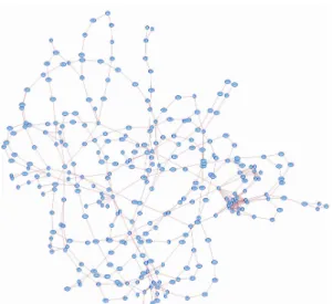
(8) random graph: c ra = k. n. central network that linked all the major parts of the Internet. The components of backbone contain “hub” nodes whose node degrees are very large. So we define the backbone as top t nodes and links on all of the shortest paths between the top t nodes. We name the filtered backbone as shortest-path subgraph. Thus, we proposed an algorithm to filter the backbones from the whole Internet map. The pseudo code is listed in Table 6.. (8). where k = 2.66 and n = 11527, thus the cra is equals to 0.0002308. The experiment result has been shown in Table 3, and the average of our sampled c values is 0.0282 (the biggest one is 0.0449 of NIC data; the smallest one is 0.0269 of random data). Comparing these two values, our value is 2 orders of magnitude larger than cra, so it’s obviously that clustering coefficient matches the small-world property.. With varied t values, we can display the filtered backbone topologies via shortest-path subgraph. Figure 8 shows the shortest-path subgraph and their all-pair shortest path length value matrix of the top 100 routers. 4 There are many cycles in above figures, as we know, IBN is not just rough hierarchical structure and will be robust under attacks or failures. Our Kf algorithm could filter the Internet backbone out efficiently.. 4.3 Geographical Visualization One of the problems faced in the analysis of Internet topology at a large-scale level consists in its map’s visualization. In general, the logical layout by two-dimensional image based on connectivity is frequently used. Figure 7 with 11,528 nodes and 12,691 links, which was drawn by a shareware, aiSee [26].. Table 6 Algorithm of filtering, Kf Input:. By visualizing the Internet, we can pick out points of the things we concern and find a closer inspection in some characteristics like clustering coefficient. Moreover, the central mesh part catches our attentions, and leads to the filtering algorithm, Kf, described in the next Subsection.. Path length matrix of all-pair shortest path: arr [maxNodes][maxNodes]; Kay matrix of all-pair shortest path: kay [maxNodes][maxNodes]; Threshold value: t, 1 ≤ t ≤ maxVertices ; Output: Adjacency matrix of Top t nodes: top[t][t]; link file: top t.txt Method: for (int i = 0; i <= t ; i++){ for (int j = 0; j <= t; j++){ top[i][j] = arr[i][j]; } } for (int i = 0; i < top.length; i++){ for (int j = 0;j < top.length; j++){ int tt = t;. Figure 7 Two-dimensional image of Internet map based on IP addresses, collected by this research. exec(int kay[i], int tt); // exec method select the whole links of i and write them to top t.txt. }. 4.4 Filtering Algorithm, Kf. }. The high variability of node degrees and the “tree-like” topology layout both indicate that the mesh part, the key feature of Figure 7, is the “core” of the Internet, or so-called Internet Backbone Networks (IBN). The Internet backbone is the. 4. 8. Of course, the real Internet backbone would be more complexity than this. Our results could be considered as an epitome of Internet..

(9) rooted tree from the maximum degree node of our sample5 and form all of the shortest paths to all the other nodes to composite a tree. Figure 9 is the shortest-path spanning tree where h is the height of the tree and its height is 23. From the viewpoint of tree structure, we consider that the smaller height of tree would decrease the whole routing distance. So that we propose to add new link to the longest path in the tree may take effects to that. Besides, randomly adding links is the “re-wiring” way used in the small-world network model, we also applied this concept to our simulations. In a word, we design two simulations based on the sampled data, the first one is called the First m Longest-Path-First method (LPF)6, and the other one is Random-Link-Added method (RLA). Furthermore, we combined the Kf algorithm with RLA method to see the simulation results with several aspects. Figure 10 is our simulation flow. The adding probability of new links, p ( 0 ≤ p ≤ 1 ), if p = 0 presents no any. Figure 8 Shortest-path subgraph of the top-100 nodes 4.5 Summary. new link be added into the network; on the contrary, when p = 1, the network will become a Kn complete graph.7 Thus, the relation between p and the number of new links, enew can be defined as. This Section reports analytical metrics of Internet topology for small-world and scale-free properties. With chi-square goodness-of-fit test, the hypothesis that the distribution of our sampled data is consistent with the population of the applied IP addresses. Our main findings are as follows. The average node degree is 2.66 and a high variability of node degree is well fitted to power-law format indicating the scale-free property in Internet. The average shortest path length is 15.1325, and the clustering coefficient is 0.0282. And these two values provide clear evidences of the presence of small-world phenomenon in Internet.. p=. enew n −e 2. (9). where n is the number of nodes and e is the number of links in the network.. Our analytical results confirm that our process is efficient to observe the Internet topology. In order to observe the changing of the Internet and obtain performance improving suggestions, we will conduct associated simulations based on our findings.. 5. Performance Simulations In order to improve the performance of the Internet, we conducted some simulations. Decreasing the path length can reduce routing cost in Internet. From the viewpoint of graph theory, the Internet is obviously in the middle of regular and random graphs. Due to the shortest path length, l of our data is from 13.75 to 15.13, still larger than the value, 9.56 of random graphs. Thus, our simulation goal is to reduce the path length. Here, we consider the hierarchal structure of the Internet with the representation of tree. We modified Dijkstra' s algorithm, which we implemented in this research to find the shortest path, to iterate on length of path to construct a shortest-path spanning tree. So we can obtain a. Figure 9 Shortest-path spanning tree of the maximum degree node. 5 6 7. The IP address is 4.68.114.157 which locates in NJ., USA and belongs to Level 3 Communications Inc We select m pairs of nodes as new links at once which their path lengths are the largest ones. A complete graph with n graph vertices is denoted Kn and has a. 9. n 2. =. n(n − 1) 2. undirected edges..

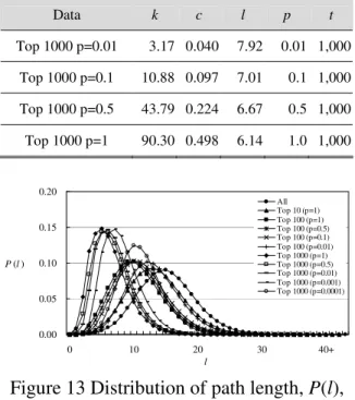
(10) Table 8 Metrics of the original union data and 3 groups by RLA Data. Figure 10 Our simulation flow. k. c. l. p. All. 2.67. 0.0272. 15.13. 0.000. LPF (p=0.001). 2.69. 0.0115. 15.13. 0.001. LPF (p=0.01). 2.71. 0.0121. 15.09. 0.010. LPF (p=0.1). 2.94. 0.0156. 14.74. 0.100. 2.67. 0.0272. 15.13. 0.000. RLA (p=0.001). 2.67. 0.0204. 15.05. 0.001. RLA (p=0.01). 2.68. 0.0268. 14.59. 0.010. RLA (p=0.1). 2.83. 0.1877. 12.07. 0.100. 0.05. 0.00 0. l. 30. 20. 30. 40+. Figure 12 Distribution of path length, P(l), for RLA algorithm Finally, we used Kf algorithm to filter out the top t subgraph of backbone. Then, combine the RLA method to generate several groups of simulations. For instance, when random adding new links to the top t subgraph with t = 100 and the probability is 10%, the path length decreases to 11.38 and the clustering coefficient arises to almost 3 times than the original data. Here, we can observe the trend of simulation results by RLA plus Kf method appears high progression. Figure 13 shows that only adding some links (with varied probability p) to major Internet backbone (the size of t) can decrease the average path length greatly. It clearly points out that our RLA plus Kf method is quite useful to reduce the path lengths.. 0.00 20. 10. l. 0.03. 10. All RLA (p=0.001) RLA (p=0.01) RLA (p=0.1). 0.10. P (l ) 0.05. 0. p. P (l ). All LPF (p=0.001) LPF (p=0.01) LPF (p=0.1). 0.08. l. 0.15. Only adds a fraction of new links, the node degree and clustering coefficient increase and the average shortest path length decreases. Figure 11 illustrates well bell-shaped distribution as our union sample. Although the trend of simulation results by LPF method appears progression, the advantage seems not so large as Table 7 shows.. 0.10. c. All. Table 7 Metrics of the original union data and 3 groups by LPF Data. k. Table 9 Metrics of the top t groups by RLA. 40+. plus Kf algorithm. Figure 11 Distribution of path length, P(l), for LPF algorithm. Data. When we use RLA method, only random adding probability of 10%, the path length decreases to 12 and the clustering coefficient arises to almost 10 times than the original data. Here, we can observe the trend of simulation results by RLA method appears large progression. Besides, Table 8 and Figure 12 show the path length rapidly decreases, which shows the amazing effect of random links.. c. l. p. t. Top 10. 2.35 0.034 13.44. 1.0. 10. Top 100 p=0.01. 2.70 0.035 13.12. 0.01. 100. Top 100 p=0.1. 2.77 0.063 11.38. 0.1. 100. Top 100 p=0.5. 2.86 0.070 10.94. 0.5. 100. Top 100 p=1. 3.14 0.120 10.53. 1.0. 100. Top 1000 p=0.001. 10. k. 2.67 0.034 11.16 0.001 1,000.

(11) Data. k. c. l. p. Top 1000 p=0.01. 3.17 0.040. 7.92. 0.01 1,000. Top 1000 p=0.1. 10.88 0.097. 7.01. 0.1 1,000. Top 1000 p=0.5. 43.79 0.224. 6.67. 0.5 1,000. Top 1000 p=1. 90.30 0.498. 6.14. 1.0 1,000. 0.20. Our main analytical results are as follows. The average node degree is 2.66 and we find the high variability of node degree distributions which follow power-law and match scale-free property. The distributions of average shortest path lengths fit well to the bell-shaped of the Poisson distribution and the mean value is 15.1325. The results confirm the small-world property of a “small” path length. We also got the clustering coefficient, 0.0282, which is 2 orders of magnitude “larger” than a random graph, that also matches the small-world property. Our observations provide clear evidence of the presence of small-world and scale-free properties in Internet topology. The analytical results provide evidences that our process is efficient to observe the Internet topology.. All Top 10 (p=1) Top 100 (p=1) Top 100 (p=0.5) Top 100 (p=0.1) Top 100 (p=0.01) Top 1000 (p=1) Top 1000 (p=0.5) Top 1000 (p=0.01) Top 1000 (p=0.001) Top 1000 (p=0.0001). 0.15 P (l ). addresses generated randomly are our sampled data. With chi-square goodness-of-fit test, the hypothesis that the distribution of our sampled data is consistent with the population of the applied IP addresses.. t. 0.10 0.05 0.00 0. 10. 20. 30. 40+. l. Figure 13 Distribution of path length, P(l), of all groups generated by RLA plus Kf algorithm. According to our simulations, we found that creating links between the longest path pair of nodes is not a useful way to improve performance; otherwise, only few percentages of random-added links can obtain a better improvement of Internet. In further thinking, the natural dynamics of the Internet should be considered and the probability of selecting new links might calculate by more parameters like the hierarchical levels, the node degrees, the latencies, and so on.. Our simulation results show that it is efficient to augment the Internet efficiency with randomly connected links. On the situation of cost constraint, we suggest just add new links randomly in the Internet. Only a very small percentage can reduce the path length. The result of RLA plus Kf simulation shows the small number of new links can reduce the path length from 15.1325 to 11.38 (See Table 9). If path length is shorter, the transportation of routing packets is less. Unfortunately, resource is often limited in real Internet world. In our experiment, we considered the subgraph of top t nodes represented to the Internet backbone, “top-100” might be a technological “sweet spot” in balancing cost and performance. If we compared 100 and the tens of millions IP addresses, 100 is small enough to be managed and coordinated. Besides, the cost is not quite heavy, when the probability of new adding links, p, is only 10%. Adding new links between such small groups is more plausibly implementable than adding between the whole Internet around the world.. Furthermore, we identified the major Internet backbone by the filtering algorithm, Kf. To further take advantage of small-world property, we suggest using random additions of extra links in Internet backbone to improve the Internet performance. By RLA plus Kf algorithm, the simulation results show that only adding 10% randomly links, 236 new links, to the backbone containing top 100 routers will decrease path length to 11.38 and increase the clustering coefficient to 0.097 as shown in Table 9. This is a technological sweet spot in balancing cost and performance. The research results can be a reference to planner and administrators of the Internet. As new technological improvements on the computer hardware, computer software, and network protocols, there are constantly changing in the Internet working. For example, the IP addresses we focused on this research are undergoing a transformation to accommodate more addresses by implementing the new IPv6 protocol. By some revising, our process still can be used to observe the new generations of Internet.. 6. Conclusions In this paper, we proposed a process to observe the Internet topology. The process offers the statistical analysis of basic metrics in topological description based on many complex network models. We sampled the Internet by several aspects, including network management, political, economic, and random sample. 191 web sites of NICs, 227 government portal sites, 500 corporations’ portal sites of 2004 Fortune Global 500, and 10 thousand IP 11.

(12) 7. Acknowledgement. and Algorithms, 1st ed. New Jersey: John Wiley & Sons, 2003.. The authors acknowledge support by the National Science Council under Grants NSC 94-2416-H-182-005.. [14]. M. Hollander and D. A. Wolfe, Nonparametric Statistical Methods, 2nd ed. New York: Wiley-Interscience, 1999.. [15]. B. Huffaker, M. Fomenkov, D. Plummer, D. Moore, and K. Claffy, “Distance Metrics in the Internet,” in Proc. IEEE International Telecommunications Symposium (ITS), Brazil, September 2002.. 8. References [1]. R. Albert, A.-L. Barabási, H. Jeong, and G. Bianconi, “Power-law distribution of the World Wide Web,” Science, vol. 287, pp. 2115a, 2000.. [16]. [2]. R. Albert, H. Jeong, and A.-L. Barabási, “Diameter of the World-Wide Web,” Nature, vol. 401, pp. 130-131, 1999.. S. Jin, Scalability of Multicast-based Streaming Delivery Mechanisms on the Internet, PhD Dissertation, Boston Univ., United States, 2003.. [17]. G. Malkin, “Traceroute Using an IP Option,” IETF, RFC 1393, 1993.. [3]. L. A. N. Amaral, A. Scala, M. Barthelemy, and H. E. Stanley, “Classes of Small-World Networks,” in Proc. National Academy of Sciences, vol. 97, no. 21, October 2000.. [18]. S. Milgram, “The Small World Problem,” Psychology Today, vol. 22, pp. 61-67, 1967.. [19]. R. Pastor-Satorras and A. Vespignani, Evolution and Structure of the Internet, 1st ed. Cambridge, UK.: Cambridge University Press, 2004.. [20]. S. Sahni, Data Structures, Algorithms, and Applications in Java, 1st ed. New York: McGraw-Hill, 2001.. [21]. R. Siamwalla, R. Sharma, and S. Keshav, “Discovering Internet Topology,” in Proc. IEEE Infocom'99, pp. 21-25, 1999.. [22]. H. Tangmunarunkit, R. Govindan, S. Jamin, S. Shenker, and W. Willinger, “Network Topology Generators: Degree based vs. Structural,” in Proc. ACM SIGCOMM 2002, 2002.. [23]. A. Vazquez, “Statistics of citation networks,” cond-mat/0105031, May 2001.. [24]. D. J. Watts and S. H. Strogatz, “Collective Dynamics of ‘Small-World’ Networks,” Nature, vol. 393, pp. 440, 1998.. [25]. S. Zhou and R. J. Mondragon, “The ‘rich-club' phenomenon in the Internet topology,” IEEE Communication Letters, November 2002.. [26]. aiSee. [Online]. Available: http://www.aisee.com. [27]. Fortune, “The 2004 Global 500: The World Largest Corporations,” 2004. [Online]. Available: http://www.fortune.com/fortune/global500. [28]. Name Intelligence, “IP Counts by Country,” 2005. [Online]. Available: http://www.whois.sc/internet-statistics/country-i p-counts.html. [29]. Root-Zone Whois Information, IANA ccTLD Database, 2004. [Online]. Available: http://www.iana.org/cctld/cctld-whois.htm. [4]. A.-L. Barabási, Linked: How Everything Is Connected to Everything Else and What It Means, 2nd ed. New York: Pub.Plume Books, 2003.. [5]. A.-L. Barabási and R. Albert, “Emergence of scaling in random networks,” Science, vol. 286, pp. 509-512, 1999.. [6]. S. Branigan, H. Burch, B. Cheswick, and F. Wojcik, “What Can You Do with Traceroute?” IEEE Internet Computing, vol. 5, no. 5, 2001.. [7]. D. S. Callaway, M. E. J. Newman, S. H. Strogatz, and D. J. Watts, “Network Robustness and Fragility: Percolation on Random Graphs,” Physical Review Letters, vol. 85, no. 25, pp. 5468, 2002.. [8]. [9]. [10]. R. F. i Cancho, C. Janssen and R. V. Sole, “Topology of technology graphs: small world patterns in electronic circuits,” Physical Review E, vol. 64, 046119, 2001. Q. Chen, H. Chang, R. Govindan, S. Jamin, S. J. Shenker and W. Willinger, “The Origin of Power Laws in Internet Topologies (Revisited),” in Proc. IEEE INFOCOM 2002, June 2002. S. Dorogovtsev and J. Mendes, Evolution of networks: from biological nets to the Internet and WWW, 1st ed. New York: Oxford University Press, 2003.. [11]. P. Erdös and A. Rényi, “On Random Graph,” Publications Mathematicae, vol. 6, pp. 290-297, 1959.. [12]. C. Faloutsos, M. Faloutsos, and P. Faloutsos, “On Power-Law Relationships of the Internet Topology,” in Proc. ACM SIGCOMM, 1999.. [13]. P. P. Frasconi and P. Smyth, Modeling the Internet and the Web: Probabilistic Methods 12.

(13)