Impacts of Transportation External Cost Pricing and Transit
Fare Reductions on Household Mode/Route Choices
and Environmental Improvements
Shwu-Ping Guo
1and Chaug-Ing Hsu
2Abstract: This study explores how transportation external cost pricing and transit fare reductions impact household mode/route choices
and environmental improvements in a metropolitan area. A household mode/route choice model and a bilevel model for transportation external cost pricing and transit fare reductions are sequentially constructed. In the first level of bilevel model, the pricing of transportation external costs, including congestion, air pollution, and noise, is measured applying the theory of marginal-cost pricing. The effects of transportation external cost pricing are analyzed in terms of variations in household mode/route choices, increased patronage of rail transit lines and reduced congestion, air pollution, and noise. In the second level of bilevel model, this study explores how to reduce rail transit fares to achieve equivalent benefits of environmental improvement as for the strategy of transportation external cost pricing. The analytical results reveal that, after the implementation of transportation external cost pricing and taxation, the number of commuting households attracted to rail transit lines will increase, and some commuting households may detour to more distant transit stations to avoid high congestion links on surface streets.
DOI: 10.1061/共ASCE兲UP.1943-5444.0000036
CE Database subject headings: Rail transportation; Costs; Pricing; Fare; Commute.
Author keywords: Rail transit system; External cost pricing; Transit fare; Mode choice.
Introduction
Transportation externalities such as congestion, air pollution, and noise, which result from the increasing use of automobiles, are unsettled and result in social costs and impaired public health in metropolitan areas. Previous studies have explored transportation externality pricing and incorporated it into the total travel costs of travelers. Some studies applied the fundamental economic prin-ciple of marginal-cost pricing to analyze the relationship between congestion toll and traffic flow, and traveler route choice behavior 共e.g., Yang and Bell 1997; Yang and Huang 1998兲. Meanwhile, dynamic models explore the influence of time-varying flows on congestion pricing and design discriminating and time-varying congestion pricing schemes during peak and off-peak periods 共e.g., Yang and Huang 1997; Daganzo and Garcia 2000兲.
Moreover, some studies adopted the economic cost perspective and applied quantitative economic approaches to construct a road pricing model that incorporates congestion, air pollution, and noise based on the marginal-cost pricing or second-best pricing methods 共e.g., Mayeres et al. 1996; Johansson 1997兲. Different
transportation supply policies also influence transportation exter-nality pricing. Therefore, some studies further analyzed transpor-tation externality pricing under different transportranspor-tation supply policies共e.g., De Borger and Wouters 1998; Romilly 1999; Ver-hoef 2000; Mayeres 2000兲. Furthermore, interactions exist be-tween transportation and environment systems. Some studies devised an integrated evaluation framework for comprehensively investigating the environmental impacts of transportation projects by applying system analysis or multicriteria analysis共e.g., Lo and Hickman 1997; Tsamboulas and Mikroudis 2000兲.
Traffic congestion is prevalent in major metropolitan areas. Rail transit and private car induce different externalities, owing to their different service attributes. The rail transit system fits envi-ronmental protection goals because it is electricity operated in three construction forms; that is, surface, at grade, and under-ground, and thus results in less pollution. Some previous studies investigated the influences of new or improved public transport systems on traveler mode and route choices, and then estimated the patronage of public transport systems共e.g., Koppelman et al. 1993; Hsu and Guo 1999兲. Previous studies have also constructed multimodal transportation networks’ models to explore passen-gers’ shifting behavior and transit fare structure共e.g., Lozano and Storchi 2001; Lo et al. 2003; Lam et al. 1999兲. This study con-siders the pricing of three transportation externalities, namely, congestion, air pollution, and noise, and incorporates them into the total travel cost function of individual travelers by applying marginal-cost pricing theory. This study constructs models to共1兲 analyze variations in household mode and route choices due to extra cost burdens from transportation externalities such as con-gestion, air pollution, and noise and 共2兲 estimate changes in the patronage of rail transit lines.
Authorities levying transportation externality taxes共e.g., con-gestion tax, air pollution tax, and noise tax兲 on surface road users 1
Associate Professor, Dept. of Logistics and Marketing Management, Leader Univ., Tainan 709, Taiwan, Republic of China 共corresponding author兲. E-mail: [email protected]
2
Professor, Dept. of Transportation Technology and Management, National Chiao Tung Univ., Hsinchu 30050, Taiwan, Republic of China. E-mail: [email protected]
Note. This manuscript was submitted on October 28, 2008; approved on April 14, 2010; published online on November 15, 2010. Discussion period open until May 1, 2011; separate discussions must be submitted for individual papers. This paper is part of the Journal of Urban Plan-ning and Development, Vol. 136, No. 4, December 1, 2010. ©ASCE, ISSN 0733-9488/2010/4-339–348/$25.00.
can be considered a strategy for encouraging public transit. In-creased total travel costs of private car users may result in private car users shifting to rail transit and consequent environmental improvements. Meanwhile, subsidies for transit operators can be transferred to passengers, thereby reducing rail transit fares and increasing the attractiveness of rail transit. Some studies analyzed the influences of bus or transit fare changes on traveler mode choice behavior, ridership, and operator revenues共e.g., Benjamin et al. 1998; Taylor and Carter 1998; Ling 1998兲. Reducing public transportation fares is a transparent strategy for travelers since it allows travelers to know their total travel costs before making their trips. This strategy is also easy to implement, particularly if it can achieve equivalent environmental improvements to the strategy of transportation external cost pricing. Consequently, this study further explores how to decrease rail transit fares at each transit line section used by commuters to travel from their homes to work to achieve equivalent environmental improvements com-pared to the strategy of transportation external cost pricing.
Household Mode and Route Choices without Considering External Cost Pricing
This study applied the continuum approximation method to as-sume the study area to be a dense network represented by a two-dimensional coordinate system D. Surface streets were assumed to be continuous and homogeneous networks, and thus the actual surface networks were not captured. The rail transit networks were represented in the form of actual networks. Let graph G共N,A兲 represent the actual rail transit network, where N denotes the set of nodes and A represents the set of links in the graph. Moreover, residential sites and rail transit stations are indicated by a two-dimensional coordinate. The main reason for applying the continuum approximation method in this study is to estimate car flows from all residential sites to each transit station using a simplified data collection process and without collecting detailed road network information. Commuting car flows generated from each residential site can be estimated based on the trip generation rate for work trip purposes at each residential site. For long-term planning purposes, this study applies a continuum approximation method to estimate commuting car flows transferring at each rail transit station.
In relation to generalized travel cost function on surface streets, this study refers to and revises the link travel time func-tion in convenfunc-tional traffic assignment models共e.g., Sheffi 1985兲 to formulate the generalized travel cost function cij共vij兲 of indi-vidual commuting households from residential site i =共i1, i2兲 to
residential site j =共j1, j2兲 via an artificial link on the surface
streets, as in Eq. 共1兲. Because commuting households pass through residential sites between their residences and workplaces, the artificial link in this study is defined as the artificial commut-ing link which connects two adjacent residential sites. To simplify the model formulation, this study assumed that each household uses a single car to commute and that workplaces of household members are highly concentrated in the central business district 共CBD兲. That is, this study explores travel patterns from numerous origins to a single destination 共CBD兲. Car pooling is commonly adopted by household members when driving to workplaces, es-pecially in a city with a large CBD
cij共vij兲 = cij0关1 + 共1 +vij/Cij兲兴 ∀ 共i, j兲 苸 F 共1兲 In Eq.共1兲, F denotes the set of all artificial links on surface streets between residential site pairs in the study area. Moreover, cij0
rep-resents the generalized travel cost which is independent of the car flows of commuting households on the artificial link from site i =共i1, i2兲 to site j=共j1, j2兲. Moreover,vij denotes the car flows of commuting households on artificial link from site i =共i1, i2兲 to site j =共j1, j2兲. Furthermore, Cij denotes the capacity of the artificial link from site i =共i1, i2兲 to site j=共j1, j2兲, and and are
param-eters. Eq.共1兲 formulates the generalized travel cost of individual households on the artificial link via surface streets. When vij is zero, i.e., free flow state, cij共0兲 not only includes the generalized travel cost of flow-independent travel time on the artificial link via surface streets, i.e., cij0, but also the out-of-packet cost, which is estimated and denoted by parameter.
Regarding the representation of rail transit networks, a transit line section is defined as a part of a rail transit route, which includes the set of all rail transit links that must be passed from a boarding station to the CBD station or a transfer station. Each rail transit line section corresponds to a rail transit station, i.e., the boarding station. Furthermore, the study of Hsu and Guo 共2001兲 defines parameters of rail transit networks as follows. Let K de-note the set of rail transit routes directly connected to the CBD without transshipment of passengers between rail transit lines. Moreover, let Kt represent the set of rail transit routes that are indirectly connected to the CBD with transshipment of passengers between rail transit lines. Passengers using rail transit routes in Kt must transship to rail transit routes in K to reach CBD. Further-more, let S denote the set of nontransferring stations while St represents the set of transfer stations. Additionally, Asis the set of rail transit line sections that directly connect to workplaces in CBD and whose initial stations are not transfer stations. Further-more, Atrepresents the set of rail transit line sections that directly connect to workplaces in CBD and whose initial stations are transfer stations. Moreover, Tsis the set of rail transit line sections that do not connect to workplaces in CBD and whose initial sta-tions are not transfer stasta-tions. Meanwhile, Tr共r苸St兲 denotes the set of rail transit line sections whose initial station is transfer station r. Additionally, Wsrepresents the set of initial stations that correspond to rail transit line sections in Asand At. Finally, Wtis the set of initial stations that correspond to rail transit line sec-tions in Ts.
The generalized travel cost tas on rail transit line section a corresponding to initial station s for an individual commuting household includes onboard time, waiting time, parking time, and fares. Owing to constant running speed, fixed frequency, and given fares of rail transit systems, the weighted sum of the on-board time and fare for rail transit line section a is assumed to be constant and is denoted by t0as. Since this study assumes work-places to be highly concentrated on the CBD, the waiting time at each rail transit station is a function of the number of boarding passengers during the peak period. Let has denote the park-and-ride car flows at rail transit station s, i.e., the initial station of rail transit line section a. Surface street flows comprise vehicles, while rail transit network flows comprise passengers. Since this study assumes all commuting members of each household to si-multaneously use the same car to travel to the CBD, the average number of commuting members per household,, also represents the average vehicle occupancy factor. Passengers at transfer sta-tions not only comprise park-and-ride travelers but also transfer from other rail transit routes that do not directly connect to the CBD. Therefore, generalized travel cost functions on rail transit line sections are constructed separately for both nontransferring stations and transferring stations and are formulated as Eqs. 共2兲 and共3兲, respectively, where ␣ and are parameters
tas共has兲 = t0as+␣共 · has/Has兲 ∀ a 苸 共As艛 Ts兲, s 苸 S 共2兲 tbr共has,hbr兲 = t0rb+␣
冋
冉
hbr+兺
a苸Tr,s苸Wt has冊
/Hbr册
∀ b 苸 At, r苸 St 共3兲This study considers traveler waiting time and parking time as delay time at their park-and-ride stations on rail transit networks. Besides passenger flows, the main determinant of traveler waiting time is available capacity of rail transit trains, while the major influence on traveler parking time is parking availability at sta-tions. Has is defined as a synthetic parameter representing the above two supply capacities at boarding station of rail transit line section a. Correspondingly, this study constructs a household mode/route choice model using Eqs. 共4兲–共10兲 including decision variables of car flows of commuting households vij on artificial link on surface streets and transferring car flows, has and hbr, to transit stations based on the principle of user equilibrium. Accord-ing to Eq.共9兲, the transferring car flows, has and hbr, can be sub-stituted by the car flows of commuting households on artificial links connected to transit stations
min TC1=
兺
共i,j兲苸F冕
0 vij cij共vij兲dvij+兺
s苸S冕
0 has tas共has兲dhas +兺
r苸St冕
0 hbr tbr共has,hbr兲dhbr 共4兲 subject to兺
j苸Di⬘ vij= gi ∀ i 苸 BF 共5兲兺
i苸Dj vij=兺
k苸D⬘j vjk ∀ j 苸 Bs ∀ i ⫽ j ⫽ k 共6兲兺
i苸Dj vij+ gj=兺
k苸D⬘j vjk ∀ j 苸 共B − BF− BS兲 ∀ i ⫽ j ⫽ k 共7兲兺
i苸Do vio+兺
s苸共S艛St兲 has=兺
j苸B gj 共8兲 has=兺
i苸Ds vis ∀ s 苸 共S 艛 St兲 共9兲 vijⱖ 0 ∀ 共i, j兲 苸 F 共10兲where gjdenotes the number of households at residential site j =共j1, j2兲; Djrepresents the set of upstream residential sites adja-cent to residential site j =共j1, j2兲; and Dj⬘= set of downstream resi-dential sites adjacent to resiresi-dential site j =共j1, j2兲. Additionally, B
denotes the set of all residential sites in the study area and BF represents the subset of residential sites located within the bound-aries of the study area; that is, BF傺B. Outflows of commuting households will only occur at residential sites of BF. BSdenotes the subset of residential sites adjacent to rail transit stations, namely, BS傺B. Eq. 共4兲 is the objective function minimizing the total generalized travel costs of commuting households on both surface streets and rail transit networks under the principle of user equilibrium. Moreover, Eqs. 共5兲–共9兲 are flow conservation con-straints at each residential site and each rail transit station in the
study area. Eq.共5兲 demonstrates that the outflows of commuting households at each residential site within the boundaries of the study area are equal to the number of households living at that residential site.
To implicitly indicate these commuting methods, the outflow of commuting households at each residential site adjacent to rail transit stations is formulated in Eq. 共6兲 as equal to the inflow of commuting households at that residential site. Commuting house-holds living at residential sites adjacent to each rail transit station generate passenger flows on the transit line section corresponding to that transit station and should be included in the generalized travel cost function on that transit line section. Restated, these passenger flows should be added to the variable has in Eq.共2兲 or Eq.共3兲, depending on whether the transit station is a nontransfer-ring or a transfernontransfer-ring station. Eq.共7兲 represents that the outflow of commuting households at each residential site, which is neither located within the boundaries of the study area nor adjacent to transit stations, should equal the inflow of commuting households at that residential site plus the number of households there. Eq. 共8兲 reveals that the total number of households living at all resi-dential sites equals the inflow of commuting households to the CBD from upstream residential sites plus the total number of transferring car flows to all of stations in the study area. Eq.共9兲 represents that car flow transferring to each transit station equals the inflow of commuting households to that station from upstream residential sites. Eq. 共10兲 is the nonnegative constraint of each decision variable.
Transportation External Cost Pricing, Transit Fare Reduction, and Household Mode/Route Choices
Household Mode/Route Choice Model Considering Transportation External Cost Pricing
This study refers to Yang and Bell 共1997兲, Yang and Huang 共1998兲, and Verhoef 共2000兲 and, besides congestion, further in-corporates transportation externalities such as air pollution and noise in formulating transportation external cost pricing and household mode/route choice model. Car flow induced congestion results in online effects on transportation networks, while the air pollution and noise induced by car flows have both online and offline effects due to the dispersion and propagation attributes of air pollution and noise, respectively. Moreover, this study as-sumes that the cost burdens of transportation externalities result-ing from rail transit systems are exempted with a lump-sum subsidy to encourage rail transit patronage. Therefore, this study neglects the pricing of transportation externalities caused by the rail transit system.
Transportation externalities such as pollution and noise are continuously dispersed and propagated over the study area. The spatial effects of pollution and noise are originally formulated using continuous functions. However, continuous spatial func-tions have difficulty calculating integrals and obtaining the opti-mal solution. Transportation studies mostly adopt a zoning method to divide the study area and then explore transportation planning issues. However, aggregation bias exists among these traffic zones. Therefore, this study applies a continuum approxi-mation method to divide the study area into discrete residential sites and formulate the external cost functions of air pollution and noise at each residential site. This study also considers the disper-sion and propagation of air pollution and noise since the offline effects of these externalities should be considered. This study
refers to Hsu and Guo共2005兲 to derive the external cost function of air pollution aex共vij兲 at residential site x=共x1, x2兲, which is
induced by the car flows of commuting households vij on the artificial link from site i =共i1, i2兲 to site j=共j1, j2兲, as expressed in
Eq.共11兲 aex共vij兲 = 1· vij· Q 2·
再
b3苸关R1,R2兴兺
1 h·z·兩w¯兩 ⫻exp冉
−1 2再
兩w¯兩2·兩i − x兩2−关共i − x兲 · w¯兴2 兩w¯兩2· h 2冎
冊
· ⫻exp冋
−1 2冉
he− b3 z冊
2册
冎
共11兲where Q denotes the emission rate per automobile andhandz represent the standard horizontal and vertical deviations of the concentration distribution, respectively. Additionally, w¯ denotes the average wind velocity vector 共w¯1, w¯2, w¯3兲. he represents the effective emission height of air pollution.关R1,R2兴 is the vertical range within which pollutants become detrimental to human health. Finally,1denotes the social cost per unit of air pollution.
Moreover, the external cost function of noise nexa共vij兲 at resi-dential site x =共x1, x2兲, which is induced by the car flows of com-muting householdsvijon the artificial link from site i =共i1, i2兲 to
site j =共j1, j2兲, is derived as Eq. 共12兲. In Eq. 共12兲, LWa represents the average sound power level 共dB re 10−12 W兲 caused by one
car. Moreover, DIa共i,x兲 denotes the directivity index of car flow noise traveling from residential site i =共i1, i2兲 to residential site x =共x1, x2兲. ⍀a共i兲 is the solid angle of car flow noise radiating
from residential site i =共i1, i2兲 and is assumed to be 2.
Further-more, Acoma 共i,x兲 is the combined attenuation index of car flow noise from site i =共i1, i2兲 to site x=共x1, x2兲. Finally, 2represents
the social cost per unit noise
nexa共vij兲 = 2·
冋
LWa ·vij− 20 log冑
共i1− x1兲2+共i2− x2兲2 1m + DI a共i,x兲 − 10 log⍀ a共i兲 4 − 11 − Acoma 共i,x兲册
共12兲This study integrates the pricing of air pollution, noise, as well as congestion on surface streets into the total generalized travel cost function of an individual commuting household on an artificial link from site i =共i1, i2兲 to site j=共j1, j2兲, which is formulated as
Eq.共13兲. This study assumes that the affected areas of air pollut-ants and noise generated from a residential site extend 3 km downwind and cover an approximately round area with a radius of 3 km. Therefore, in Eq.共13兲, Bijaeand Bijne, respectively, denote the sets of residential sites affected by air pollutants and noise induced by the car flows of commuting households on the artifi-cial link from site i =共i1, i2兲 to site j=共j1, j2兲. The third and fourth
components of the right-hand side of Eq.共13兲, respectively, rep-resent the marginal-cost burdens of air pollution and noise created in additional households tcijsur共vij兲 = cij共vij兲 +vij· dcij共vij兲 dvij +vij· d
关
兺
x苸B ij aeaex共vij兲兴
dvij +vij· d关
兺
x苸B ij nenexa共vij兲兴
dvij ∀ 共i, j兲 苸 F 共13兲 This study constructs a transportation external cost pricing and household mode/route choice model, shown as Eqs.共14兲 and 共15兲.Eq.共14兲 is the objective function for minimizing the total gener-alized travel costs of commuting households. Set SSvin Eq.共15兲 represents the solution set of decision variables and comprises Eqs.共5兲–共10兲 min TC2=
兺
共i,j兲苸F冕
0 vij tcijsur共vij兲dvij+兺
s苸S冕
0 has tas共has兲dhas +兺
r苸St冕
0 hbr tb r共h a s ,hb r兲dh b r 共14兲 subject to vij苸 SSv ∀ 共i, j兲 苸 F 共15兲 This study further compares the results of the two models con-structed here for estimating the benefits due to transportation ex-ternal cost pricing in terms of the generalized travel cost saving and external cost reductions of air pollution and noise. The ag-gregated benefit after the implementation of transportation exter-nal cost pricing and taxation is derived as Eq.共16兲BF共vij1,vij2兲 =
兺
共i,j兲苸F 关vij1· cij共vij1兲 −vij2· cij共vij2兲兴 +兺
s苸S艛St 关h1a s· t a s共h1 a s兲 − h2 a s· t a s共h2 a s兲兴 +兺
共i,j兲苸Fx兺
苸B 关aex共vij1兲 − aex共vij2兲兴 +兺
共i,j兲苸Fx兺
苸B 关nex共vij1兲 − nex共vij 2兲兴 共16兲wherevij1 andvij2 denote the car flows of commuting households on an artificial link on surface streets from site i =共i1, i2兲 to site j =共j1, j2兲, respectively, in the household mode/route choice model
both with and without considering the transportation external cost pricing, while h1as and h2as represent the car flows of commuting households transferring at rail transit station s, respectively, in the above two models.
Household Mode/Route Choice Model Considering Transit Fare Reductions
In the second-level programming model, this study establishes a household mode/route choice model that considers transit fare reductions, with the aim of minimizing the generalized travel costs of individual households and with the constraint of achiev-ing environmental improvements equivalent to those achieved by the strategy of transportation external cost pricing and taxation. The proposed idea is based on the following reasons. First, the pricing of transportation external costs is both difficult to deter-mine and hard for citizens to realize. Additionally, the strategy of transportation external cost pricing is treated as punishment for ill behavior and is not welcomed by citizens. This study thus pro-poses a method of reducing transit fares to achieve equivalent environmental improvement benefits to the strategy of transporta-tion external cost pricing. Transit fares are more transparent to citizens. However, the question of who will pay for fare reduc-tions is also significant. To be fair, fair reducreduc-tions might be imple-mented by the government levying a fuel tax on car users and then subsidizing transit operators. Levying a fuel tax offers a practical way to internalize some transportation externalities based on the principle of user charge. Furthermore, if citizens know that some fuel tax revenues are used to reduce transit fares,
their complaints will be reduced. The idea and results proposed in this study can also provide a reference to authorities for designing environmental improvement strategies.
The decision variables used in the second-level model include car flow of commuting householdsvij on each artificial link on surface streets and the transit fare pason rail transit line section a corresponding to initial station s. Herein, the transit fare pas is extracted from the constant parameter t0as, which was defined as the weighted sum of onboard time and fare in Eqs.共2兲 and 共3兲, for rail transit line section a. The generalized travel cost functions on rail transit line sections for nontransferring stations and transfer-ring stations, respectively, are reformulated as Eqs.共17兲 and 共18兲. Meanwhile, t0a⬘s and t0b⬘r denote the generalized travel costs of onboard time on rail transit line sections for nontransferring sta-tions and transferring stasta-tions, respectively.
ta⬘s共has, pas兲 = t0a⬘s+ pas+␣共 · has/Has兲 ∀ a 苸 共As艛 Ts兲, s 苸 S 共17兲 tb⬘r共has,hbr, pas兲 = t0⬘br+ pas+␣
冋
冉
hbr+兺
a苸Tr,s苸Wt has冊
/Hbr册
∀ b 苸 At, r苸 St 共18兲Furthermore, this study compares the results of the household mode/route choice model with and without considering transit fare reductions. The aggregated benefit after the implementation of transit fare reductions is then formulated as Eq.共19兲 in terms of the generalized travel cost saving and external cost reductions associated with air pollution and noise
BF共vij1,vij3兲 =
兺
共i,j兲苸F关 vij1· cij共vij 1兲 −v ij 3· c ij共vij 3兲兴 +兺
s苸S艛St 关h1as· tas共h1as兲 − h3as· ta⬘ s共h3 a s, p a s兲兴 +兺
共i,j兲苸Fx兺
苸B 关aex共vij 1兲 − ae x共vij 3兲兴 +兺
共i,j兲苸Fx兺
苸B 关nex共vij 1兲 − ne x共vij 3兲兴 共19兲where vij3 denotes the car flow of commuting households on an artificial link on surface streets from site i =共i1, i2兲 to site j
=共j1, j2兲 in the household mode and route choice model
consid-ering transit fare reductions and h3asrepresents the park-and-ride car flow at rail transit station s, which is the initial station of rail transit line section a, in the household mode/route choice model considering transit fare reductions.
According to the above derivations, this study constructs a household mode/route choice model that considers transit fare reductions as Eqs. 共20兲–共22兲. Eq. 共20兲 is the objective function which minimizes the generalized travel cost of individual com-muting household. Eq.共21兲 is the same as Eq. 共15兲. Meanwhile, Eq. 共22兲 demonstrates that the aggregated benefit due to the implementation of transportation external cost pricing and taxa-tion equals that of transit fare reductaxa-tions
min vij,has,hbr,pas TC3=
兺
共i,j兲苸F冕
0 vij cij共vij兲dvij+兺
s苸S冕
0 has ta⬘s共has, pas兲dhas +兺
r苸St冕
0 hbr tb⬘r共has,hbr, pas兲dhbr 共20兲 subject to vij苸 SSv ∀ 共i, j兲 苸 F 共21兲 BF共vij1,vij2兲 = BF共vij1,vij3兲 共22兲 Problem-Solving ProcedureTo facilitate problem solving, this study applies the Lagrangian multiplier to relax the constraints of the three models and rewrites them as three Lagrangian functions, L1, L2, and L3, and their
corresponding Lagrangian multipliers, mr, Or, and fr. The Karush-Kuhn-Tucker optimality conditions are then derived for each Lagrangian function to determine the solutions of the deci-sion variables. The solution steps involved in applying the Newton-Raphson’s method for the models constructed here are clarified as follows.
Step 1. Set k = 0. Determine initial values for the decision
vari-ables and Lagrangian multipliers. Set the maximal number of it-erations K = 120.
Step 2. Generate Jacobian matrices associated with the three
sets of nonlinear simultaneous equations in the kth iteration.
Step 3. The increased 共or decreased兲 values for the decision
variables and Lagrangian multipliers of the three minimization problems are calculated during the kth iteration.
Step 4. Design a safeguard process to prevent divergent
solu-tions. The variations between iterations may occasionally cause divergent solutions in cases where current approximate solutions are overshot. The safeguard process attempts to smoothly adjust variations eventuating from Step 3 and to induce search directions toward an equilibrium. This step restricts the percentage of varia-tions in the kth iteration values of all decision variables and La-grangian multipliers from exceeding 20% of the k − 1th iteration values.
Step 5. Approximate numerical solutions for the 共k+1兲th
it-eration. Set k = k + 1.
Step 6. If current solutions for the three minimization
prob-lems satisfy convergent conditions, stop the problem solving pro-cedure and output the results. Otherwise, go to Step 7. The convergent conditions are satisfied and equilibrium solutions are obtained when the percentage variation in the value of each itera-tion for each decision variable is below 10%.
Step 7. If the number of iterations reaches maximum, go to
Step 8. Otherwise, go to Step 2.
Step 8. Design a flow conservation inspection process to
en-sure that the constraints are satisfied. If not all constraints are satisfied, this study sequentially adjusts the corresponding car flows of commuting households for each unsatisfied constraint. Finally, the results are outputted.
Example
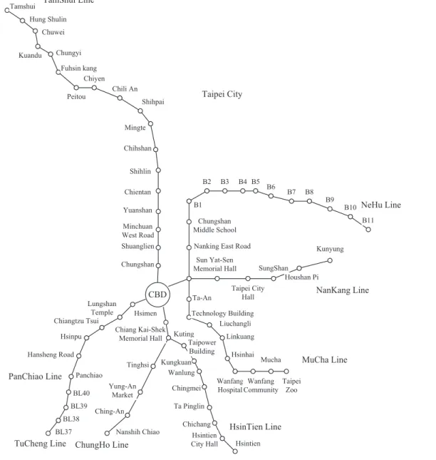
This study adopts the Taipei metropolitan area covered by the Taipei Mass Transit System, which is shown as Fig. 1, to
strate the feasibility of applying the proposed models. To reduce the problem scale and facilitate problem solving procedures, tran-sit stations with spacings of less than 1 km are consolidated and the rail transit networks are simplified. The study area is repre-sented by a graph with 214 nodes共residential sites兲 and 340 arti-ficial links, which connect two adjacent residential sites. In terms of generalized travel cost function on an artificial link, the range of Cij, i.e., the capacity of artificial link from site i =共i1, i2兲 to site j =共j1, j2兲, is assumed to be 关25, 120兴 共unit: thousands兲. The het-erogeneity of artificial link capacity is simulated by generating random variables with respect to locations of residential sites. The generalized travel cost, cij0, which is independent of the car flows of commuting households on the artificial link from site i =共i1, i2兲 to site j=共j1, j2兲 is converted from the travel time using
the value of time. The value of cij0is estimated based on the length of the artificial link and the assumed parameters, such as the value of time of NT$7.0/min and the average speed of 35 km/h. More-over, to facilitate problem solving and convergence, the values of parameters and are assumed to be 0.18 and 4.0, respectively. Regarding generalized travel cost on a transit line section and the external cost functions of air pollution and noise, this study refers
to the parameter values in Hsu and Guo共2001, 2005兲. Household Mode/Route Choices before and after Transportation External Cost Pricing
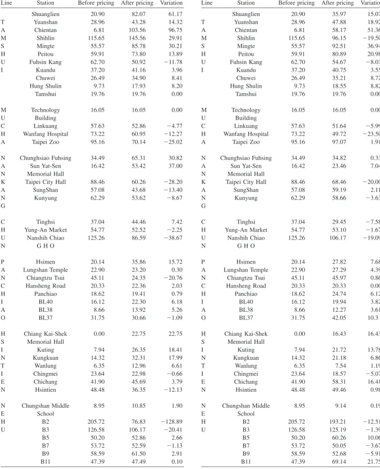
This study explored the influences of transportation external cost pricing and taxation on the mode/route choices of commuting households without considering the offline effects of these exter-nalities. These results are shown in Table 1 and reveal that more commuting households are willing to shift to rail transit lines when offline effects of transportation external costs are incorpo-rated. A possible reason for this situation is that external costs of air pollution and noise, induced by car flows passing through each residential site, cumulatively influence other residential sites in the study area. Therefore, the pricing of transportation external costs considering offline effects is higher than that without con-sidering offline effects. More car flows of commuting households travel to transit stations.
Variations in the car flows of commuting households transfer-ring at transit stations before and after transportation external cost pricing are summarized in Table 2. These results indicate that CBD NeHu Line NanKang Line MuCha Line HsinTien Line ChungHo Line TuCheng Line PanChiao Line TamShui Line Taipei City Ta-An Technology Building Liuchangli Linkuang Wanfang Hospital Wanfang Community Hsinhai Mucha Taipei Zoo Lungshan Temple Chiangtzu Tsui Hsinpu Hansheng Road Panchiao BL40 BL39 BL38 BL37 Hsimen Sun Yat-Sen Memorial Hall Taipei City Hall SungShan Houshan Pi Kunyung Chungshan Shuanglien Minchuan West Road Yuanshan Chientan Shihlin Chihshan Mingte Shihpai Chili An Chiyen Peitou Fuhsin kang Chungyi Kuandu Chuwei Hung Shulin Tamshui Chiang Kai-Shek Memorial Hall Kuting
Taipower Building Kungkuan Wanlung Chingmei Ta Pinglin Chichang Hsintien
City Hall Hsintien Tinghsi
Yung-An Market Ching-An
Nanshih Chiao
Nanking East Road Chungshan Middle School B1 B2 B3 B4 B5 B6 B7 B8 B9 B10 B11
Fig. 1. Diagram of study area
Table 1. Car Flows Transferring at Transit Stations before and after
Transportation External Cost Pricing without Considering Offline Effects 共Unit: 1,000 Households兲
Line Station Before pricing After pricing Variation
Shuanglien 20.90 82.07 61.17 T Yuanshan 28.96 43.28 14.32 A Chientan 6.81 103.56 96.75 M Shihlin 115.65 145.56 29.91 S Mingte 55.57 85.78 30.21 H Peitou 59.91 73.80 13.89 U Fuhsin Kang 62.70 50.92 ⫺11.78 I Kuandu 37.20 41.16 3.96 Chuwei 26.49 34.90 8.41 Hung Shulin 9.73 17.93 8.20 Tamshui 19.76 19.76 0.00 M Technology 16.05 16.05 0.00 U Building C Linkuang 57.63 52.86 ⫺4.77 H Wanfang Hospital 73.22 60.95 ⫺12.27 A Taipei Zoo 95.16 70.14 ⫺25.02 N Chunghsiao Fuhsing 34.49 65.31 30.82 A Sun Yat-Sen 16.42 53.42 37.00 N Memorial Hall
K Taipei City Hall 88.46 60.26 ⫺28.20
A SungShan 57.08 43.68 ⫺13.40 N Kunyung 62.29 53.62 ⫺8.67 G C Tinghsi 37.04 44.46 7.42 H Yung-An Market 54.77 52.52 ⫺2.25 U Nanshih Chiao 125.26 86.59 ⫺38.67 N G H O P Hsimen 20.14 35.86 15.72 A Lungshan Temple 22.90 23.20 0.30 N Chiangtzu Tsui 45.11 24.35 ⫺20.76 C Hansheng Road 20.33 22.36 2.03 H Panchiao 18.62 19.41 0.79 I BL40 16.12 22.30 6.18 A BL38 8.66 13.92 5.26 O BL37 31.75 30.66 ⫺1.09 H Chiang Kai-Shek 0.00 22.75 22.75 S Memorial Hall I Kuting 7.94 26.35 18.41 N Kungkuan 14.32 32.31 17.99 T Wanlung 6.35 12.96 6.61 I Chingmei 23.64 22.98 ⫺0.66 E Chichang 41.90 45.69 3.79 N Hsintien 48.48 36.35 ⫺12.13 N Chungshan Middle 8.95 10.85 1.90 E School H B2 205.72 76.83 ⫺128.89 U B3 126.58 106.17 ⫺20.41 B5 50.20 52.86 2.66 B7 53.72 52.59 ⫺1.13 B9 58.59 61.50 2.91 B11 47.39 47.49 0.10
Table 2. Car Flows Transferring at Transit Stations before and after
Transportation External Cost Pricing with Considering Offline Effects 共Unit: 1,000 Households兲
Line Station Before pricing After pricing Variation
Shuanglien 20.90 35.97 15.07 T Yuanshan 28.96 47.88 18.92 A Chientan 6.81 58.17 51.36 M Shihlin 115.65 96.15 ⫺19.50 S Mingte 55.57 92.51 36.94 H Peitou 59.91 80.89 20.98 U Fuhsin Kang 62.70 54.67 ⫺8.03 I Kuandu 37.20 40.75 3.55 Chuwei 26.49 35.21 8.72 Hung Shulin 9.73 18.55 8.82 Tamshui 19.76 19.76 0.00 M Technology 16.05 16.05 0.00 U Building C Linkuang 57.63 51.64 ⫺5.99 H Wanfang Hospital 73.22 49.72 ⫺23.50 A Taipei Zoo 95.16 97.07 1.91 N Chunghsiao Fuhsing 34.49 34.82 0.33 A Sun Yat-Sen 16.42 23.46 7.04 N Memorial Hall
K Taipei City Hall 88.46 68.46 ⫺20.00
A SungShan 57.08 59.19 2.11 N Kunyung 62.29 58.66 ⫺3.63 G C Tinghsi 37.04 29.45 ⫺7.58 H Yung-An Market 54.77 53.10 ⫺1.67 U Nanshih Chiao 125.26 106.17 ⫺19.09 N G H O P Hsimen 20.14 27.82 7.68 A Lungshan Temple 22.90 27.29 4.39 N Chiangtzu Tsui 45.11 45.97 0.86 C Hansheng Road 20.33 20.33 0.00 H Panchiao 18.62 24.74 6.12 I BL40 16.12 19.94 3.82 A BL38 8.66 12.27 3.61 O BL37 31.75 42.05 10.3 H Chiang Kai-Shek 0.00 16.43 16.43 S Memorial Hall I Kuting 7.94 21.72 13.78 N Kungkuan 14.32 21.18 6.86 T Wanlung 6.35 7.54 1.19 I Chingmei 23.64 18.57 ⫺5.07 E Chichang 41.90 58.31 16.41 N Hsintien 48.48 49.46 0.98 N Chungshan Middle 8.95 9.14 0.19 E School H B2 205.72 193.21 ⫺12.51 U B3 126.58 125.19 ⫺1.39 B5 50.20 60.26 10.06 B7 53.72 50.05 ⫺3.67 B9 58.59 52.68 ⫺5.91 B11 47.39 69.14 21.75
commuting households attracted to the Tamshui, Panchiao, and Hsintien Lines will increase after the implementation of transpor-tation external cost pricing and taxation. Regarding the competi-tion among rail transit lines, some commuting households originally transferring to the Chungho Line will shift to stations along the Hsintien and Panchiao Lines. Comparing Tables 1 and 2 reveals that due to offline effects of transportation external costs, car flows of commuting households transferring to transit stations increase with total generalized travel costs on artificial links via surface streets. However, the increases are not significant.
Distributions of Transportation External Cost Pricing Fig. 2 illustrates the distribution of air pollution and noise pricing in the study area after the implementation of transportation exter-nal cost pricing and taxation. The results indicate that situations involving high air pollution and noise pricing mainly occur in areas near the CBD and around the transit stations along the Chungho, Hsintien, and Mucha Lines. Finally, the results shown in Fig. 2 also provide a reference for future studies in designing the pricing system of transportation external costs.
For estimating the benefits of environmental improvement, this study assumes the benefits per household per day,1and2,
which resulted from 1,000-g reductions of cumulative air pollu-tion and 1,000-dB共A兲 reductions of cumulative noise, respec-tively, to be US$1.834⫻10−5and US$0.912⫻10−5by referring
to Aunan et al. 共1998兲 and Otterstrom 共1995兲. Furthermore, ac-cording to Eq.共16兲, the total environmental improvements due to transportation external cost pricing and taxation in the study area are estimated to be NT$1,574,472/day. Therein, the total general-ized travel cost saving is NT$301,867/day, and the savings from reductions in air and noise pollution are NT$1,135,646/day and NT$136,959/day, respectively.
Result Analysis after Considering Transit Fare Reductions
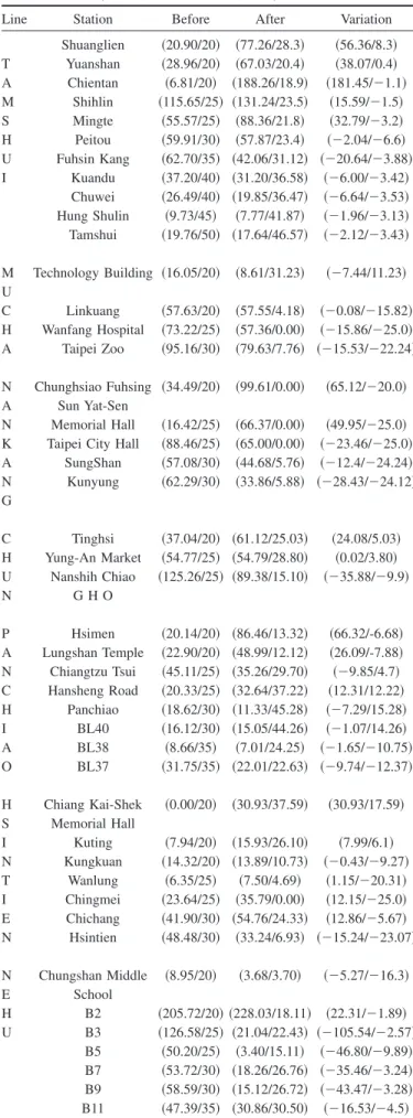
Table 3 summarizes variations in both car flows of commuting households transferring at transit stations and fares on transit line sections before and after transit fare reductions. Initially, transit fares are expected to display an overall reduction to achieve the benefits of environmental improvement compared with the
strat-Table 3. Car Flows and Fares at Transit Stations before and after Transit
Fare Reductions共Unit: 1,000 Households; NT$兲
Line Station Before After Variation
Shuanglien 共20.90/20兲 共77.26/28.3兲 共56.36/8.3兲 T Yuanshan 共28.96/20兲 共67.03/20.4兲 共38.07/0.4兲 A Chientan 共6.81/20兲 共188.26/18.9兲 共181.45/⫺1.1兲 M Shihlin 共115.65/25兲 共131.24/23.5兲 共15.59/⫺1.5兲 S Mingte 共55.57/25兲 共88.36/21.8兲 共32.79/⫺3.2兲 H Peitou 共59.91/30兲 共57.87/23.4兲 共⫺2.04/⫺6.6兲 U Fuhsin Kang 共62.70/35兲 共42.06/31.12兲 共⫺20.64/⫺3.88兲 I Kuandu 共37.20/40兲 共31.20/36.58兲 共⫺6.00/⫺3.42兲 Chuwei 共26.49/40兲 共19.85/36.47兲 共⫺6.64/⫺3.53兲 Hung Shulin 共9.73/45兲 共7.77/41.87兲 共⫺1.96/⫺3.13兲 Tamshui 共19.76/50兲 共17.64/46.57兲 共⫺2.12/⫺3.43兲 M Technology Building 共16.05/20兲 共8.61/31.23兲 共⫺7.44/11.23兲 U C Linkuang 共57.63/20兲 共57.55/4.18兲 共⫺0.08/⫺15.82兲 H Wanfang Hospital 共73.22/25兲 共57.36/0.00兲 共⫺15.86/⫺25.0兲 A Taipei Zoo 共95.16/30兲 共79.63/7.76兲 共⫺15.53/⫺22.24兲 N Chunghsiao Fuhsing 共34.49/20兲 共99.61/0.00兲 共65.12/⫺20.0兲 A Sun Yat-Sen N Memorial Hall 共16.42/25兲 共66.37/0.00兲 共49.95/⫺25.0兲 K Taipei City Hall 共88.46/25兲 共65.00/0.00兲 共⫺23.46/⫺25.0兲 A SungShan 共57.08/30兲 共44.68/5.76兲 共⫺12.4/⫺24.24兲 N Kunyung 共62.29/30兲 共33.86/5.88兲 共⫺28.43/⫺24.12兲 G C Tinghsi 共37.04/20兲 共61.12/25.03兲 共24.08/5.03兲 H Yung-An Market 共54.77/25兲 共54.79/28.80兲 共0.02/3.80兲 U Nanshih Chiao 共125.26/25兲 共89.38/15.10兲 共⫺35.88/⫺9.9兲 N G H O P Hsimen 共20.14/20兲 共86.46/13.32兲 共66.32/-6.68兲 A Lungshan Temple 共22.90/20兲 共48.99/12.12兲 共26.09/-7.88兲 N Chiangtzu Tsui 共45.11/25兲 共35.26/29.70兲 共⫺9.85/4.7兲 C Hansheng Road 共20.33/25兲 共32.64/37.22兲 共12.31/12.22兲 H Panchiao 共18.62/30兲 共11.33/45.28兲 共⫺7.29/15.28兲 I BL40 共16.12/30兲 共15.05/44.26兲 共⫺1.07/14.26兲 A BL38 共8.66/35兲 共7.01/24.25兲 共⫺1.65/⫺10.75兲 O BL37 共31.75/35兲 共22.01/22.63兲 共⫺9.74/⫺12.37兲 H Chiang Kai-Shek 共0.00/20兲 共30.93/37.59兲 共30.93/17.59兲 S Memorial Hall I Kuting 共7.94/20兲 共15.93/26.10兲 共7.99/6.1兲 N Kungkuan 共14.32/20兲 共13.89/10.73兲 共⫺0.43/⫺9.27兲 T Wanlung 共6.35/25兲 共7.50/4.69兲 共1.15/⫺20.31兲 I Chingmei 共23.64/25兲 共35.79/0.00兲 共12.15/⫺25.0兲 E Chichang 共41.90/30兲 共54.76/24.33兲 共12.86/⫺5.67兲 N Hsintien 共48.48/30兲 共33.24/6.93兲 共⫺15.24/⫺23.07兲 N Chungshan Middle 共8.95/20兲 共3.68/3.70兲 共⫺5.27/⫺16.3兲 E School H B2 共205.72/20兲 共228.03/18.11兲 共22.31/⫺1.89兲 U B3 共126.58/25兲 共21.04/22.43兲 共⫺105.54/⫺2.57兲 B5 共50.20/25兲 共3.40/15.11兲 共⫺46.80/⫺9.89兲 B7 共53.72/30兲 共18.26/26.76兲 共⫺35.46/⫺3.24兲 B9 共58.59/30兲 共15.12/26.72兲 共⫺43.47/⫺3.28兲 B11 共47.39/35兲 共30.86/30.50兲 共⫺16.53/⫺4.5兲 0 50 100 0 50 100 150 0 20 40 60 80 x-coordinate y-coordinate pri c ing of ai r p o ll u ti o n an d n oi s e (N T $ )
Fig. 2. Pricing of air pollution and noise—results of households’
mode/route choice model with considering transportation external
cost pricing共unit: NT$兲
egy of transportation external cost pricing. However, the results in Table 3 illustrate increased transit fares from some stations near the CBD, such as Shuanglien and Yuanshan on the Tamshui Line, Technology Building on the Mucha Line, Chiang Kai-Shek Me-morial Hall, and Kuting on the Hsintien Line. This situation may occur because congestion on artificial links via surface streets intensifies with closeness to the CBD; therefore, fares from transit stations near the CBD rise sufficiently to restrain overflow of transferring commuting households. Namely, the degree of transit fare reduction increases with increasing distance from the board-ing station to the CBD, thus attractboard-ing commutboard-ing households to transfer at transit stations near their residential sites. These situa-tions occur at transit stasitua-tions such as Wanfang Hospital and Taipei Zoo on the Mucha Line, and B38 and B37 on the Panchiao Line. Regarding car flow variations, commuting households transfer-ring at some transit stations increase after transit fare reductions; however, numbers of transferring commuting households de-crease at certain transit stations. This situation may occur due to the waiting time at transit stations; thus some commuting house-holds prefer to drive by car via surface streets to the CBD for minimizing their generalized travel costs.
Conclusions and Suggestions
This study from the long-term planning perspective applies a con-tinuum approximation method to develop static and deterministic models for exploring commuter mode/route choice behavior. Two policies for encouraging rail transit system; i.e., internalized transportation external costs and transit fare reductions, are pro-posed to analyze the influences on commuter mode/route choice behavior. Two major assumptions are assumed in this study. First, this study applies the continuum approximation method to assume the study area to be a dense network represented by a two-dimensional coordinate system. Second, this study assumes that each household uses a single car to commute and that the work-places of household members are highly concentrated in the CBD. That is, this study explores patterns of travel from many origins to a single destination 共CBD兲. The main results of the models are共1兲 the variation in the patronage of each transit sta-tion before and after transportasta-tion external cost pricing and tran-sit fare reductions and 共2兲 fare reductions at each transit station. The results related to fare reductions at each station can provide a guide for implementing a fare reduction scheme and thus can not only efficiently attract more passengers but can also effectively reduce externalities. Furthermore, results related to the variation in patronage can reveal which transit stations attract more patron-age after transportation external cost pricing or transit fare reduc-tions. The analytical results can also assist transit operators in planning facility capacity, adjusting schedules, and determining transit fares.
However, the proposed models have some limitations in po-tential applications for analyzing real-world issues. In respect to the applications of case studies, future studies should explore the influences of different temporal patterns of trip generation on the pricing of transportation externalities. Furthermore, this study adopts a metropolitan example and assumes that workplaces are highly concentrated in the CBD to simplify the model formula-tion. Future studies should extend to a multicentric urban configu-ration involving multiple mode/route alternatives to investigate the modal split for all available modes and optimize public trans-portation network fare structure. Since real-world situations are too complicated for model construction, future studies exploring
real-world issues can select several major work centers to analyze commuter mode/route choice behavior and the influences of tran-sit fare reductions by applying the model proposed here. The results of multiple travel patterns involving many origins to a single destination can then be combined. Third, to implement practical studies for operating purposes, future studies should apply actual road networks to indicate link flows. To explore the spatial effects of air pollution and noise, future studies could also apply geographic information system technology to obtain precise data from various locations. Fourth, since traffic congestion and the resultant noise and air pollution are correlated, adding them together as independent terms for the total generalized travel cost function might overestimate the total external costs. Future stud-ies can further consider the correlated effects among external costs. Finally, commuting households may change their residence after the implementation of transportation external cost pricing. Future studies can construct an interaction model with mode/route choices and residence choices to explore household migration be-havior before and after transportation external cost pricing.
Acknowledgments
The writers would like to thank the National Science Council of the Republic of China for financially supporting this research under Contract No. NSC91-2415-H-009-004.
References
Benjamin, J., Kurauchi, S., Morikawa, T., Polydoropoulou, A., Sasaki, K., and Ben-Akiva, M. 共1998兲. “Forecasting paratransit ridership using discrete choice models with explicit consideration of availabil-ity.” Transp. Res. Rec., 1618, 60–65.
Daganzo, C. F., and Garcia, R. C.共2000兲. “A Pareto improving strategy for the time-dependent morning commute problem.” Transp. Sci.,
34共3兲, 303–311.
De Borger, B., and Wouters, S.共1998兲. “Transport externalities and op-timal pricing and supply decisions in urban transportation: A simula-tion analysis for Belgium.” Reg. Sci. Urban Econ., 28, 163–197. Hsu, C. I., and Guo, S. P.共1999兲. “Access mode combinations for
inter-city transportation terminals in a metropolitan area.” Journal of the
Eastern Asia Society for Transportation Studies, 3共2兲, 333–348.
Hsu, C. I., and Guo, S. P. 共2001兲. “Household-mode choice and residential-rent distribution in a metropolitan area with surface road and rail transit networks.” Envir. Plan. A, 33共9兲, 1547–1575. Hsu, C. I., and Guo, S. P.共2005兲. “Externality reductions in residential
areas due to rail transit networks.” Ann. Reg. Sci., 38, 1–12. Johansson, O.共1997兲. “Optimal road-pricing: Simultaneous treatment of
time losses, increased fuel consumption and emissions.” Transp. Res.
D, 2共2兲, 77–87.
Koppelman, F. S., Bhat, C. R., and Schofer, J. L. 共1993兲. “Market-research evaluation of actions to reduce suburban traffic congestion— Commuter travel behavior and response to demand reduction actions.” Transp. Res., Part A: Policy Pract., 27共5兲, 383–393. Lam, W. H. K., et al.共1999兲. “A stochastic user equilibrium assignment
model for congested transit networks.” Transp. Res., Part B:
Meth-odol., 33, 351–368.
Ling, J. H.共1998兲. “Transit fare differentials: A theoretical analysis.” J.
Adv. Transp., 32共3兲, 297–314.
Lo, H. K., and Hickman, M. D. 共1997兲. “Toward an evaluation frame-work for road pricing.” J. Transp. Eng., 123共4兲, 316–324.
Lo, H. K., Yip, C. W., and Wan, K. H.共2003兲. “Modeling transfer and non-linear fare structure in multi-modal network.” Transp. Res., Part
B: Methodol., 37, 149–170.
Lozano, A., and Storchi, G.共2001兲. “Shortest viable path algorithm in
multimodal networks.” Transp. Res., Part A: Policy Pract., 35, 225– 241.
Mayeres, I. 共2000兲. “The efficiency effects of transport policies in the presence of externalities and distortionary taxes.” J. Transp. Econ.
Policy, 34共2兲, 233–260.
Mayeres, I., Ochelen, S., and Proost, S.共1996兲. “The marginal external costs of urban transport.” Transp. Res. D, 1共2兲, 111–130.
Romilly, P.共1999兲. “Substitution of bus for car travel in urban Britain: An economic evaluation of bus and car exhaust emission and other costs.” Transp. Res. D, 4, 109–125.
Sheffi, Y. 共1985兲. Urban transportation networks: Equilibrium analysis
with mathematical programming methods, Prentice-Hall, Englewood
Cliffs, N.J.
Taylor, S. R. W., and Carter, D. W.共1998兲. “Maryland mass transit ad-ministration fare simplification-effects on ridership and revenue.”
Transp. Res. Rec., 1618, 125–130.
Tsamboulas, D., and Mikroudis, G.共2000兲. “EFECT—Evaluation frame-work of environmental impacts and costs of transport initiatives.”
Transp. Res. D, 5, 283–303.
Verhoef, E. T. 共2000兲. “The implementation of marginal external cost pricing in road transport.” Papers in Regional Science, 79, 307–332. Yang, H., and Bell, M. G. H.共1997兲. “Traffic restraint, road pricing and network equilibrium.” Transp. Res., Part B: Methodol., 31共4兲, 303– 314.
Yang, H., and Huang, H. J.共1997兲. “Analysis of the time-varying pricing of a bottleneck with elastic demand using optimal control theory.”
Transp. Res., Part B: Methodol., 31共6兲, 425–440.
Yang, H., and Huang, H. J.共1998兲. “Principle of marginal-cost pricing: How does it work in a general road network.” Transp. Res., Part A:
Policy Pract., 32共1兲, 45–54.