Hybrid adaptive block truncation coding for image compression

Hybrid adaptive block truncation coding for

image compression

Ching-Yung Yang Ja-Chen Lin

National Chiao Tung University Institute of Computer and Information

Science

Hsinchu, Taiwan 300 E-mail: [email protected]

Abstract. A hybrid adaptive block truncation coding (HABTC) method is

presented to improve block truncation coding (BTC)-related compression methods for gray-level images. The basic idea behind the method is to use various coding schemes to take advantage of local image charac-teristics. A simple linear interpolation coding scheme and a very basic predictive coding scheme are used to improve the compression ratio of the homogeneous area of the image. Moreover, a four-level BTC, whose thresholds are obtained using a radius-weighted mean (RWM), is ap-plied to encode the inhomogeneous area. The bits per pixel/peak SNR (bpp/PSNR) values listed in many other BTC-related papers are cited and compared with ours. It is found that reasonable compression ratio is obtained by the proposed HABTC method and the visual quality of the decoded images is also acceptable. © 1997 Society of Photo-Optical Instrumen-tation Engineers. [S0091-3286(97)00104-9]

Subject terms: image compression; hybrid adaptive block truncation coding; lin-ear interpolation coding; predictive coding; radius weighted mean; vector quanti-zation.

Paper 05036 received Mar. 2, 1996; revised manuscript received Sep. 11, 1996; accepted for publication Sep. 12, 1996.

1 Introduction

Block truncation coding~BTC! is a simple lossy compres-sion technique for digitized images. The main drawback of the conventional BTC algorithm is its relatively high bit rate~for example, 2 bits/pixel if each block is of size 434!. Although the compression ratio of the BTC algorithm is inferior to other block-based encoding methods, such as the transform coding1 and vector quantization2 ~VQ! tech-niques, BTC gained popularity due to its practical useful-ness. Since the BTC algorithm was first introduced by Delp and Mitchell3 in 1979, it has been modified in various ways. Based on the preservation of the first sample moment and the first absolute central moment, Lema and Mitchell4 proposed the absolute moment BTC ~AMBTC! algorithm to lower the bits per pixel~bpp! required by BTC. Udpikar and Raina5 also developed a fast implementation approach to BTC with performance similar to that of the AMBTC. To reduce the bit rate further, Udpikar and Raina6applied the VQ technique to quantize the BTC encoding results; either the bitmap vectors or the gray-level vectors~or both! are quantized. When both are quantized, the bpp is 1.0 if both codebooks have size 256. Efrati et al.7 presented the BTC-classification VQ ~BTC-CVQ! technique that com-bines the classification technique of vector quantization with the BTC algorithm. The visual quality of the decoded image was substantially improved, but the coding effi-ciency was restricted to a moderate bit rate ~usually 1.50 bpp!. Wu and Coll8 quantized the BTC coding results by applying VQ to the bitmap, and the discrete cosine trans-form ~DCT! to the high- and low-mean subimages. Their BTC-VQ-DCT, when applied to the image ‘‘Lena,’’ had a peak SNR~PSNR! value 30.56 at 0.6875 bpp.

From the preceding review, we can see that the resulting bit rate produced by these modified versions of the BTC algorithms are still not good. In this paper, we therefore try to improve the bit rate of the BTC algorithm by combining some other techniques with BTC. To achieve this goal, we take advantage of the well-known fact that most natural images can be segmented into regions of widely varying perceptual importance.7 A linear interpolation coding scheme and a predictive coding scheme are applied to en-code the homogeneous blocks of which the gray values vary constantly. As for the inhomogeneous blocks, we quantize the gray values in each block into four levels by using a four-level radius-weighted mean ~RWM! BTC modified from the conventional two-level BTC.

This paper is organized as follows. In Sec. 2, we de-scribe the proposed hybrid adaptive block truncation cod-ing~HABTC! for image compression. An optional version HABTC-VQ, which enhances HABTC with VQ, is also provided in Sec. 2.2.2. Simulation results are presented in Sec. 3. The compression performance of the proposed HABTC method is compared there with those of the other BTC-related methods, including the AMBTC, BTC-CVQ, VQ-interpolative BTC~VQ-IBTC! ~Ref. 9!, VQ-BTC ~Ref. 10!, hybrid VQ ~HVQ! ~Ref. 11!, BTC-VQ-DCT, etc. Sec-tion 4 concludes the paper.

2 Proposed HABTC Method

Let an input image be partitioned into nonoverlapping blocks of size 434. Each block is first classified into a homogeneous block or an inhomogeneous block according to the statistical characteristics of that block. More pre-cisely, a block is judged to be homogeneous if and only if

the standard deviationsof the gray values of the block is less than a threshold value T_s. Blocks that are not homo-geneous will be referred to as inhomohomo-geneous blocks. To code effectively, the homogeneous blocks are classified fur-ther into three categories, namely, interpolatable blocks, predictive blocks, and uniform blocks. Homogeneous blocks are transmitted using quite few bits. As for inhomo-geneous blocks, they are quantized using a four-level BTC. To transmit the 32-bit allocation map generated by this four-level BTC, there are two versions: without VQ or with VQ. Usually, the version without VQ is suggested, unless a bpp lower than 0.57 is expected. Note that without VQ means that the original 32-bit map is transmitted directly. As for the version with VQ, we divide the inhomogeneous blocks into edge blocks and texture blocks depending on whether or not they contain edges. Then, a texture code-book is used to imitate the maps of texture blocks, and four edge codebooks~horizontal, vertical, diagonal, and antidi-agonal, respectively! are used to imitate the maps of edge blocks. Traditionally, whether a block contains edges or not can be known by applying a standard edge detection opera-tor such as the Sobel or Prewitt operaopera-tor. In this paper, however, we use a faster and simpler approach suggested by Dondes and Rosenfeld12 by measuring the minimum total variation ~MTV! of the block. Note that the MTV measure is also capable of detecting the four kinds of the orientations~that is, horizontal, vertical, diagonal, and an-tidiagonal! of the edge existing in the edge blocks. To

im-prove clarity, the scheme of the proposed HABTC is de-scribed in Fig. 1. The details are explained in the next two subsections.

2.1 Homogeneous Block Coding

Since most of the improved versions of the BTC algorithms are still inefficient for coding homogeneous blocks, we try to use as few bits as possible to represent these blocks. To achieve this goal, three effective techniques called linear interpolation coding, predictive coding, and uniform coding are employed in our method to encode the homogeneous blocks. To increase the compression efficiency without de-grading the visual quality too much in the encoding of a homogeneous block, the sequence of the linear interpola-tion coding test, predictive coding test, and uniform coding process appearing in Fig. 1 are best not changed.~We had tried to switch the sequence of the linear interpolation cod-ing test with the predictive test, and it was found that al-though the compression ratio increased a little, the PSNR of the reconstructed images degraded somewhat too much.! 2.1.1 Part I: the bunch of interpolatable blocks For each scan line of the blocks~that is, the blocks located in the same row!, if there are a series of homogeneous blocks connected together and if the difference between the means of each two adjacent blocks is almost constant~the variation of the differences is below a certain threshold Ti!,

then we can use an interpolation technique to quantize the blocks. The interpolation policy is illustrated in Fig. 2. Without loss of generality, let B₁,B₂,...,B_kdenote a series of homogeneous blocks that are adjacent to one another, and let their corresponding means be y₁, y₂,..., y_k, respec-tively. If y22y1'y32y2'y42y3'•••'yk2yk21, that

is, if the means change at a rate that is almost constant, then we may estimate the values yp by

yp'y

8

p5y11~p21!3s ;2<p<k21, ~1!

where s is a slope defined by Fig. 1 Scheme of the proposed HABTC method.

Fig. 2 Decoding of the homogeneous blocks$B₂,B₃,...,B_k21% us-ing the meansy1andykof blocksB1andBk[see Eqs. (1) and (2)].

s5yk2y1

k21 . ~2!

Since there are three kinds of homogeneous blocks to be encoded in our HABTC method, we use three category indices $10;11;01% to distinguish them ~the category index 00 is reserved for inhomogeneous blocks!. The kind of block discussed in this paragraph uses 10 as its category index. In other words, for the k blocks B1,B2,...,Bk, we

transmit only the sequence $(10),y₁,k22,y_k%, where 10 stands for category classification, and k22 denotes the number of ‘‘intermediate’’ blocks$B₂,B₃,...,B_k21%whose means are not transmitted and thus will require the help of Eqs.~1! and ~2! to recover. The receiver then uses Eqs. ~1! and ~2! to obtain $y₁,y₂

8

,y₃

8

,..., y_k

8

₂₁,y_k% before using these~exact or approximated! means to reconstruct homo-geneous blocks B1through Bk. In this example, the bunch

of the k blocks B₁,B₂,...,B_kare referred to as the interpo-latable blocks, because we do not transmit means y2 to

y_k21, but instead, we interpolate y₁ and y_k to obtain the estimated values y₂

8

to y_k

8

₂₁ for the intermediate blocks. The number of bits required to encode the whole bunch of the k blocks$B₁,B₂,...,B_k% is only 21. That is, 2 bits for the category classification, 16 bits for the mean value of blocks B₁and B_kat the two ends, and 3 bits to record k22, i.e., to record the length of the intermediate blocks. @We have assumed that 1<k22<8523, i.e., 3<k<10, because a large value of k ~more than 10! is seldom encountered in the real applications.#

2.1.2 Part II: predictive blocks

For the predictive blocks, nothing but the category classi-fication bits are transmitted. The reconstructed mean yˆ_{i, j}of the block is obtained by a commonly seen formula: yˆ_{i, j}50.75yˆ_{i, j21}20.5yˆ_i21,j2110.75yˆ_i21,j, ~3! where yˆ_{i, j21}, yˆ_i21,j21, and yˆ_i21,j, are the reconstructed means~can either be lossless or lossy! of the left neighbor, upper-left neighbor, and upper neighbor of the block (i, j ), respectively. In other words, the mean of the predictive blocks can not be reconstructed without the help of its three neighboring blocks. Consequently, there are only 2 bits ~be-cause the category index of the predictive block is 11! re-quired to encode a predictive block. To avoid the severe degradation, the estimated mean yˆ_{i, j} of the block is tested against the true mean yi, j each time to determine whether

the predictive coding approach should be applied or not. 2.1.3 Part III: uniform blocks

Finally, a homogeneous block that cannot be encoded by either the interpolation coding or predicting coding tech-nique is referred to as the smooth block. Since the gray values do not vary much inside the blocks, it is intuitive that the block can be represented by its mean. Instead of using 8 bits to encode the smooth block, we use 5 bits ~uniform quantizer! to quantize the mean of the block so as to reduce the bit rate. The coding format of the smooth block is $~01!,yq%, where 01 indicates the ‘‘smooth’’

cat-egory of the block. The number of bits used to encode a smooth block is therefore 7. Note that only 5 bits are used

to generate the 32-level uniform quantization needed here, although in Sec. 2.1.1 either y1 or yk did use the finer

256-gray-level system because the precision of the y₁ and yk values will affect further the gray values of some other

blocks B₂ to B_k21.

2.2 Inhomogeneous Block Coding

2.2.1 Four-level BTC using RWM

The 434516 gray values g₁ to g₁₆ of an inhomogeneous block are quantized to four levels x¯_ll, x¯_lh, x¯_hl, and x¯_hh according to the following procedure. First, we use the RWM~Ref. 13! of G5$g1...g16%as the bisection threshold

to split G into two subsets L and H. Then the RWM of L is used to split L into two smaller subsets LL and LH. Simi-larly, the RWM of H is used to split H into two smaller subsets HL and HH. Now, the average of the gray values falling in LL is computed and called as x¯_ll. Analogous statements hold for x¯_lh, x¯_hl, and x¯_hh. Since the 434 block is quantized to four levels, each pixel i will need 2 bits to indicate which of the four levels is used to replace the gray values gi. Therefore, an allocation map of 23~434!532

bits is needed to indicate the spatial allocation of the four levels. As for the four representation gray values $¯x_ll,x¯_lh,x¯_hl,x¯_hh% themselves, to increase the compression ratio, instead of transmitting these four values directly, we transmit the$a,d,d_h,d_l% defined by

a5~x¯hh1x¯hl!/41~x¯lh1x¯ll!/4, ~4!

d5~x¯hh1x¯hl!/42~x¯lh1x¯ll!/4, ~5!

dh5~x¯hh2x¯hl!/2, ~6!

and

dl5~x¯lh2x¯ll!/2. ~7!

With the definition ofa,d,dh, anddl just given, it is easy

to prove thata1d6d_hgives us x¯_hhand x¯_hl, whilea2d6d_l gives us x¯_lhand x¯_ll. In this paper, we quantizea,d,dh, and

dl to, respectively, 6, 5, 4, and 4 bits. Therefore, an

inho-mogeneous block is transmitted as $~00!;a,d,dh,dl; 32-bit

allocation map% using 21~6151414!12~434!553 bits. Here, 00 is the category index for inhomogeneous blocks.

In the preceding paragraph, the reason that RWM was used was because RWM can bisect a data set into two classes more efficiently than many other kinds of bisection methods do. To show this, we performed an extra experi-ment. Suppose that each of the 512/43512/4 blocks is to be quantized into two levels.~In other words, temporarily as-sume that two-level BTC is to be used throughout the whole image.! Then, it can be seen from the middle column of Table 1 that obtaining optimal14bisection threshold for each block is time-consuming. However, from the right-most column of Table 1, we can see that using RWM as the bisection threshold can give a nearly optimal PSNR within a short processing time.

2.2.2 HABTC-VQ (the optional version with VQ) If we want to increase the compression ratio further, then the 32-bit allocation map of each inhomogeneous block can

be quantized using fewer bits by the VQ technique. But this quantization is not suitable if high PSNR~such as 38 dB for ‘‘Lena’’! is desired. In fact, our experience told us that, if the compression ratio is lower than 14~or equivalently, if bpp is higher than 0.57!, then using the version with VQ is not worthy, because the PSNR is degraded too much by VQ for compression ratio falling in the low range.

The version with VQ, called as HABTC-VQ, is intro-duced here. Note that, to reduce the time needed to find the nearest code word from the codebook, we do not suggest the use of a single codebook for all inhomogeneous blocks. Instead, the inhomogeneous blocks are classified further as edge blocks and texture blocks. Each of these two catego-ries has its own codebook. The detail are as follows. Part I: texture blocks. An inhomogeneous block con-tains no edge is classified as a texture block.~In Part II, we introduce how to use MTV to distinguish edge blocks from texture blocks.! In HABTC-VQ, a texture codebook of size 21051024 is used to reproduce approximately the 32-bit allocation map for each texture block. Therefore, the

en-coding sequence for a texture block is

$(000);a,d,dh,dl;It%. Here, 000 denotes that the

inhomo-geneous block is in fact a texture block, (a,d,d_h,d_l) are as stated in Sec. 2.2.1, and It is the index used to obtain the

texture-map pattern selected from the texture codebook. The number of bits required to encode a texture block is 31~6151414!110532.

Part II: edge blocks. An inhomogeneous block is clas-sified as an edge block if only if the MTV of the block is greater than a predetermined threshold value T_m.~An in-homogeneous block that is not an edge block is then called a texture block.! Without loss of generality, let the 434 gray values of an inhomogeneous block be as shown in Fig. 3. The measure of the MTV is defined by

MTV5uHTV2mu1uVTV2mu1uDTV2mu

1uADTV2mu, ~8!

where m5~HTV1VTV1DTV1ADTV!/4. Here, HTV, VTV, DTV, and ADTV denote the variations along the horizontal, vertical, diagonal, and antidiagonal directions, respectively. They are defined as follows~see Fig. 3!:

HTV5~ua2b1ub2cu1uc2du1ue2 fu1uf 2gu1ug2hu

1ui2 ju1uj2ku1uk2lu1um2nu1un2ou

1uo2pu!/12, ~9!

VTV5~ua2eu1ue2iu1ui2mu1ub2 fu1uf 2 ju 1uj2nu1uc2gu1ug2ku1uk2ou1ud2hu

1uh2lu1ul2pu!/12, ~10!

DTV5~ub2eu1uc2 fu1uf 2iu1ud2gu1ug2 ju

1uj2mu1uh2ku1uk2nu1ul2ou!/9, ~11!

and

ADTV5~uc2hu1ub2gu1ug2lu1ua2 fu1uf 2ku

1uk2pu1ue2 ju1uj2ou1ui2nu!/9. ~12!

Experimental evidence12 indicates that the technique for measuring the MTV can detect not only the existence of the edges, but also the orientations of the edges. According to the orientation of edges, we have four kinds of edge-codebooks, namely, horizontal, vertical, diagonal, and an-tidiagonal. Each of these four codebooks has size 295512, and each code word is a typical 32-bit allocation map for some edge blocks. Therefore, the coding sequence of the edge blocks is $(001);a,d,dh,dl;Ce,Ie%. Here, 001

de-notes that the inhomogeneous block is in fact an edge block; (a,d,dh,dl) are as stated in Sec. 2.2.1; Ceis a 2-bit

index used to distinguish the four possible edge-codebooks; and Ie is a 9-bit index used to indicate the 512 possible

code words kept in the edge-codebook identified by C_e. The number of bits required to encode an edge blocks is therefore 31~6151414!1219533 bits.

Fig. 3 Inhomogeneous block with 16-pixel gray values [see Eqs. (9)

to (12)].

3 Experimental Results

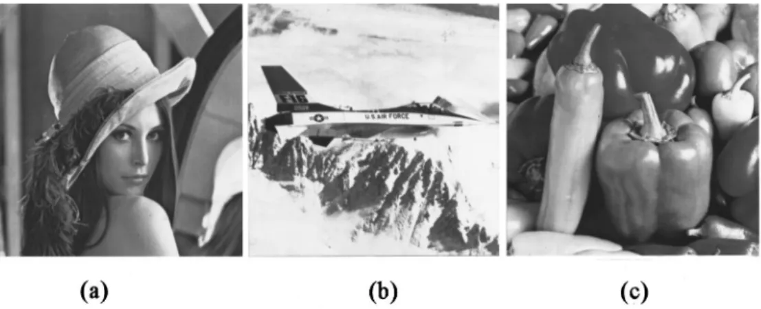
The proposed HABTC method was implemented on a Sun SPARC 10 workstation. Three 5123512 gray-scale images with 8 bpp, as shown in Fig. 4, namely, ‘‘Lena,’’ ‘‘Jet,’’ and ‘‘Peppers,’’ were tested. Many researchers used the PSNR as a measuring tool to gauge the image quality. The PSNR is defined as

PSNR5103log10

2552

MSE~dB!, ~13!

where the MSE is the mean square error. Although the PSNR does not correlate quite well with the perceived im-age quality, it does provide some information of the relative performance. We therefore use it in this section. A simple smoothing procedure was applied to the decoded images to alleviate somewhat the blocking effects that exhibit in the homogeneous regions of the images. Compressed images of ‘‘Lena,’’ ‘‘Jet,’’ and ‘‘Peppers’’ at 0.52 bpp are given in Fig. 5.

Since our method is a BTC-related hybrid method that uses classification skill ~according to the local statistics of each block!, we compared our results with some other

BTC-related hybrid methods @VQ-IBTC ~Ref. 9!, BTC-CVQ~Ref. 7!, HVQ ~Ref. 11!, adaptive compression cod-ing ~ACC! ~Ref. 15!, BTC-VQ-DCT ~Ref. 8!, VQ-BTC ~Ref. 10!, PDPCM-BTC ~Ref. 16!, and block pattern VQ ~BPVQ! ~Ref. 17!# and classified methods @BTC-CVQ, CVQ in DCT domain ~Ref. 18!, ACC, HVQ#. All data listed in Tables 2 to 4 for the reported methods are cited from the original papers~the only exception is the data for AMBTC, which were the simulation results quoted from Ref. 15!. The reason that Table 2 is longer than Tables 3 and 4 is that the image ‘‘Lena’’ was used by more research-ers in their reported papresearch-ers than the images ‘‘Jet’’ and ‘‘Peppers’’ were. As for our method, the results about HABTC are provided from high bpp through low bpp, whereas the results about HABTC-VQ~the entries marked with an asterisk! are provided for low bpp only ~because we had stated that the version with VQ is not worthy for high bpp!. It is obvious that the proposed method can obtain higher PSNR by a bpp lower than the bpp needed by these BTC-related methods.

4 Conclusions

We have presented a hybrid compression technique, the HABTC method, to improve the bit rate of the BTC algo-rithm by incorporating some recently developed tech-Fig. 4 Three original images: (a) ‘‘Lena,’’ (b) ‘‘Jet,’’ and (c) ‘‘Peppers.’’

Fig. 5 Reconstructed images of the proposed HABTC method at 0.52 bpp: (a) ‘‘Lena’’ (32.28 in PSNR), (b) ‘‘Jet’’

niques. Homogeneous blocks of the images are processed by the interpolation coding, predictive coding, or the uni-form coding techniques to reduce the bit rate greatly. Inho-mogeneous blocks are handled using four-level BTC whose thresholds are determined by the RWM bisection tool. Ex-perimental results show that the compression ratios and PSNR values of the proposed method outperform those of many other BTC-related methods.~For the image ‘‘Lena,’’ the PSNR value is about 31 when the bit rate is 0.37 bpp.! Acknowledgments

This work was supported by the National Science Council, Republic of China, under grant NSC85-2213-E009-111. References

1. M. Rabbani and P. W. Jones, ‘‘Transform coding,’’ Chap. 10 in Digi-tal Image Compression Techniques, pp. 102–128, SPIE Optical En-gineering Press, Bellingham, WA~1991!.

2. N. M. Nasrabadi and R. A. King, ‘‘Image coding using vector quan-tization: a review,’’ IEEE Trans. Commun. 36~8!, 957–971 ~1988!. 3. E. J. Delp and O. R. Mitchell, ‘‘Image compression using block

trun-cation coding,’’ IEEE Trans. Commun. 27~1!, 1335–1342 ~1979!. 4. M. D. Lema and O. R. Mitchell, ‘‘Absolute moment block truncation

coding and application to color image,’’ IEEE Trans. Commun. 32~10!, 1148–1157 ~1984!.

5. V. R. Udpikar and J. P. Raina, ‘‘Modified algorithm for block trun-cation coding of monochrome images,’’ Electron. Lett. 21~20!, 900– 902~1985!.

6. V. R. Udpikar and J. P. Raina, ‘‘BTC image coding using vector quantization,’’ IEEE Trans. Commun. 35~3!, 352–356 ~1987!. 7. N. Efrati, H. Liciztin, and H. B. Mitchell, ‘‘Classified block truncation

coding-vector quantization: an edge sensitive image compression al-gorithm,’’ Signal Process. Image Commun. 3, 275–283~1991!. 8. Y. Wu and D. C. Coll, ‘‘BTC-VQ-DCT hybrid coding of digital

im-ages,’’ IEEE Trans. Commun. 39~9!, 1283–1287 ~1991!.

9. B. Zeng and Y. Neuvo, ‘‘Interpolative BTC image coding with vector quantization,’’ IEEE Trans. Commun. 41~10!, 1436–1438 ~1993!. 10. S. A. Mohamed and M. M. Fahmy, ‘‘Image compression using

VQ-BTC,’’ IEEE Trans. Commun. 43~7!, 2177–2182 ~1995!.

11. K. A. Wen and C. Y. Lu, ‘‘Hybrid vector quantization,’’ Opt. Eng. 32~7!, 1496–1502 ~1993!.

12. P. A. Dondes and A. Rosenfeld, ‘‘Pixel classification based on gray level and local business,’’ IEEE Trans. Pattern Anal. Mach. Intell. 4~1!, 79–84 ~1982!.

13. C. Y. Yang and J. C. Lin, ‘‘Use of radius weighted mean to cluster

Table 2 Results generated by HABTC and other existing methods

on the image ‘‘Lena.’’

bpp PSNR for HABTC PSNR for Existing Methods

2.11 38.09

1.63 31.73 (AMBTC; Refs. 4 and 15)

1.5 34.85 (PDPCM-BTC; Ref. 16) 1.46 30.22 (BTC-CVQ; Ref. 7) 1.36 33.37 (ACC; Ref. 15) 1.3125 33.07 (BTC-VQ-DCT; Ref. 8) 1.25 36.24 33.01 (ACC; Ref. 15) 1.0 30.36 (PDPCM-BTC; Ref. 16) 1.0 30.59 (VQ-IBTC; Ref. 9) 0.99 33.98 (HQBPVQ; Ref. 17) 0.875 31.81 (BTC-VQ-DCT; Ref. 8) 0.83 34.44 0.836 33.21 (VQ-BTC; Ref. 10) 0.813 32.57 (CVQ in DCT domain; Ref. 18) 0.8125 31.98 (BTC-VQ-DCT; Ref. 8) 0.76 28.95 (ACC; Ref. 15) 0.75 31.21 (BTC-VQ-DCT; Ref. 8) 0.75 32.23 (CVQ in DCT domain; Ref. 18) 0.75 29.30 (VQ-IBTC; Ref. 9) 0.715 32.81 (VQ-BTC; Ref. 10) 0.71 33.77 0.6875 30.56 (BTC-VQ-DCT; Ref. 8) 0.625 31.26 (CVQ in DCT domain; Ref. 18) 0.62 33.18 0.52 30.95 (BPVQ; Ref. 17) 0.48 32.01/32.32* 0.398 29.52 (HVQ; Ref. 11) 0.37 30.87/31.35*

*_{HABTC-VQ, i.e., the HABTC equipped with VQ.}

Table 3 Results generated by HABTC and other existing methods

on the image ‘‘Jet.’’

bpp PSNR for HABTC PSNR for Existing Methods

1.71 38.01

1.63 30.48 (AMBTC; Refs. 4 and 15)

1.5 34.03 (PDPCM-BTC; Ref. 16) 1.33 37.30 1.21 33.06 (ACC; Ref. 15) 1.14 34.87 (ACC; Ref. 15) 1.13 36.45 1.0 28.96 (PDPCM-BTC; Ref. 16) 0.95 33.08 (HQBPVQ; Ref. 17) 0.872 33.51 (VQ-BTC; Ref. 10) 0.81 31.18 (ACC; Ref. 15) 0.76 33.85 0.51 29.88 (BPVQ; Ref. 17) 0.50 30.73/31.47* 0.41 29.06 (HVQ; Ref. 11) 0.39 29.10/29.96*

*_{HABTC-VQ, i.e., the HABTC equipped with VQ.}

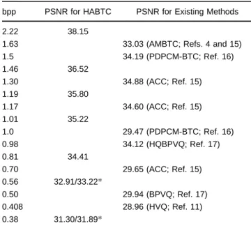
Table 4 Results generated by HABTC and other existing methods

on the image ‘‘Peppers.’’

bpp PSNR for HABTC PSNR for Existing Methods

2.22 38.15

1.63 33.03 (AMBTC; Refs. 4 and 15)

1.5 34.19 (PDPCM-BTC; Ref. 16) 1.46 36.52 1.30 34.88 (ACC; Ref. 15) 1.19 35.80 1.17 34.60 (ACC; Ref. 15) 1.01 35.22 1.0 29.47 (PDPCM-BTC; Ref. 16) 0.98 34.12 (HQBPVQ; Ref. 17) 0.81 34.41 0.70 29.65 (ACC; Ref. 15) 0.56 32.91/33.22* 0.50 29.94 (BPVQ; Ref. 17) 0.408 28.96 (HVQ; Ref. 11) 0.38 31.30/31.89*

two-class data,’’ Electron. Lett. 30~10!, 757–759 ~1994!.

14. M. Kamel, C. T. Sun, and L. Guan, ‘‘Image compression by variable block truncation coding with optimal threshold,’’ IEEE Trans. Image Process. 39~1!, 208–212 ~1991!.

15. P. Nasiopoulos, R. K. Ward, and D. J. Morse, ‘‘Adaptive compression coding,’’ IEEE Trans. Commun. 39~8!, 1245–1254 ~1991!. 16. C. H. Chen and C. F. Chen, ‘‘Progressive DPCM system with block

truncation coding,’’ Electron. Lett. 31~21!, 1821–1822 ~1995!. 17. S. A. Mohamed and M. M. Fahmy, ‘‘Image compression using block

pattern-vector quantization,’’ Signal Process. 34~1!, 69–84 ~1993!. 18. D. S. Kim and S. U. Lee, ‘‘Image vector quantizer based on a

classi-fication in the DCT domain,’’ IEEE Trans. Commun. 39~4!, 549–556

~1991!.

Ching-Yung Yang received his BS in

elec-tronic engineering in 1983 from National Taiwan Institute of Technology and his MS in electrical engineering in 1990 from Na-tional Cheng Kung University, Taiwan. From 1986 to 1988, he was a mainte-nance engineer at Central Taiwan Tele-communication Administration of the Min-istry of Transportation and Commun-ication, Taiwan. In 1992 he joined the Computer Vision Laboratory of the Depart-ment of Computer and Information Science at National Chiao Tung

University, where he is currently a PhD candidate. His recent re-search interests include pattern recognition, image compression, and vector quantization. Mr. Yang is a member of the Chinese Im-age Processing and the Pattern Recognition Society.

Ja-Chen Lin received his BS in computer

science in 1977 and his MS in applied mathematics in 1979, both from National Chiao Tung University, Taiwan. In 1988 he received his PhD in mathematics from Purdue University. From 1981 to 1982, he was an instructor at National Chiao Tung University. From 1984 to 1988, he was a graduate instructor at Purdue University. In August 1988 he joined the Department of Computer and Information Science at National Chiao Tung University, where he is currently a professor. His recent research interests include pattern recognition, image pro-cessing, and parallel computing. Dr. Lin is a member of the Phi-Tau-Phi Scholastic Honor Society, the Image Processing and Pattern Recognition Society, and the IEEE Computer Society.