相關性隱藏節點與學習演算法

(1)

行政院國家科學委員會專題研究計畫成果報告

研究成果報告(精簡版)

計畫類別：個別型計畫編號： NSC 95-2416-H-004-049- 執行期間： 95 年 08 月 01 日至 96 年 07 月 31 日執行單位：國立政治大學資訊管理學系計畫主持人：蔡瑞煌計畫參與人員：學士級-專任助理：楊佳鳳報告附件：出席國際會議研究心得報告及發表論文處理方式：本計畫可公開查詢

中華民國 96 年 07 月 30 日

(2)

I

1. The Construction Procedure

Huang and Babri (1998) propose an elegant construction method to set up a real-valued single-hidden layer feed-forward neural network (SLFN) with N hidden nodes that successfully learns N distinct samples with zero error. In a correlated real-valued single-hidden layer feed-forward neural network (SLFN), the weight vectors in the input layer of all its hidden nodes are linearly dependent. Tsaih and Wan (2007) realize that the SLFN constructed by Huang and Babri (1998) is correlated. They further show that the correlated SLFN has the property of hyperplane preimages. The correlated SLFN provides a hyperplane-preimage approach for the nonlinear regression problem with the assumption of linear preimage. Such usages motivate a study of the construction procedure for creating a correlated SLFN with less than N hidden nodes that perfectly fits N distinct samples.

The proposed construction procedure will initially set up one hidden node and then recruit (add) more (linearly dependent) hidden nodes during the learning process. In the literature, there are some similar procedures; for instance, the tiling algorithm for binary-valued layered feed-forward neural networks (cf. Me’zard and Nadal, 1989), the cascade-correlation algorithm (cf. Fahlman and C. Lebiere, 1990), and the upstart algorithm for binary-valued layered feed-forward neural networks (cf. Frean, 1990). In contrast to these researches, this study copes with the correlated real-valued SLFN.

In the context of estimation, the response y equates f(x, w) + δ where w is the parameter vector and δ is the error term. Usually, the function form of f is predetermined and fixed during the process of deriving its associated w from a given data set of observations {(1x, 1y), …, (Nx, Ny)}, with cy being the observed response corresponding to the cth observation cx.

The least squares estimator (LSE) is one of the most popular methods for estimating. If wˆ denotes any estimate of w, then LSE is defined to minimize

N c 1=

∑ce2, where

ce = cy - f(cx, wˆ ). (1)

The generalized delta rule proposed in (Rumelhart, Hilton, and Williams, 1986) for the learning process of SLFN is a kind of (nonlinear) LSE. The LSE, however, is known to be very sensitive to outliers.

In the literature of linear regression analysis, there are two approaches of dealing with outlier problems: deletion diagnostics and robust estimators (cf. Rousseeuw and Leroy (1987, page 8)). The diagnostic approach assesses the influence of an individual observation or a subset of observations to the LSE. The diagnostic approach is useful to assess the adequacy of the underlying assumption and to identify unexpected characteristics of the data. One way for the diagnostics is to identify the observations that leave the largest change in the diagnostic quantity (cf. (Cook and Weisberg, 1982)(Atkinson, 1985)) when they are excluded from the fitted data set.

As for the robust statistics approach, the robustness analysis (cf. (Hampel, 1986)) limits the attention to a “trimmed” sum of squared residuals instead of adding all the squared residuals as in the LSE. If only the first q of those ordered squared residuals are included in the summation, then the least trimmed squares (LTS) estimator is defined as

Minimize

q c 1=

(3)

where [c]e2 denotes the ordered squared residuals; that is, [1]e2 ≤ [2]e2 ≤ …≤ [N]e2. Zaman,

Rousseeuw, and Orthan (2001) suggest that ⎣0.75N⎦1

is a reasonable value for q in most empirical studies.

Atkinson and Cheng (1999) adapt the forward search algorithm proposed in (Atkinson, 1994) to develop the LTS estimates. The forward search algorithm consists of randomly adopting an (initial) subset of m+1 observations to fit the linear regression model, ordering the residuals of all N observations, and then augmenting the subset gradually by including extra observations based upon the smallest squared residuals principle.

The C-step2 of Rousseeuw and Van Driessen (2002) can release quite fast a series of subsets of observations whose corresponding total squared residuals are refined gradually. The last subset results in a good linear fitting function which is an approximation of the LTS estimator.

2. The Mapping Requirement and Notations

An SLFN provides a nonlinear mapping between x and y, whose form is y = f(x). f is a nonlinear function whose parameters (i.e., weights and biases) are derived from a given data set of mapping samples {(x1, t1), …, (xN, tN)} with xc1 ≠ xc2, c

1 ≠ c2, and with tc the target

value of y corresponding to xc. x ≡ (x1, x2,…, xm)T ∈ Rm where xj is the jth input component, with j from 1 to m.

Hereafter, m and p denote the numbers of adopted input and hidden nodes, respectively;

2 0

j

w stands for the bias of the jth hidden node; 2

j w ≡ (w2_j₁, 2 2 j w , …, 2 jm

w )T for the weights between the jth hidden node and input layer; 3

0

w for the bias of the output node; and _w3≡

( 3 1 w , 3 2 w , …, 3 p

w )T for the weights between the output node and all hidden nodes. Characters in bold represent column vectors; the superscript T indicates transposition.

Let the tanh(t) activation function be used by all hidden nodes and a linear activation function be used by the output node. Thus, given the cth sample xc, the activation value of the

jth hidden node ac( 2 0

j

w , 2

j

w ) and the output value yc are as follows:

ac( 2 0 j w , 2 j w ) ≡ tanh(w2_j₀+m i 1= ∑ 2 ji w xic); (3) yc ≡ 3 0 w + p j 1= Σ 3 j w ac( 2 0 j w , 2 j w ). (4)

Given the N mapping samples, let v( 2

0 j w , 2 j w ) ≡ (a1( 2 0 j w , 2 j w ), a2( 2 0 j w , 2 j w ), …, aN( 2 0 j w , 2 j

w ))T ∈ (-1,1)N be the responding vector of the jth hidden node with the cth component being ac( 2

0

j

w , 2

j

w ). Furthermore, let 1 be a N × 1 vector with all components 1 and T ≡ (t1, t2, …, tN)T∈ RN. Thus, the set of simultaneous equations 3

0 w + p j 1= Σ 3 j w tanh( 2 0 j w +m i 1= ∑ 2 ji w c i

x ) = tc ∀ c = 1, …, N is equivalent to system (5), which states that T is in the space spanned by 1 and p responding vectors, {v( 2

0 j w , 2 j w ), j = 1, …, p}. 3 0 w 1 + p j 1= Σ 3 j w v( 2 0 j w , 2 j w ) = T. (5)

1_Hereafter,_{⎣x⎦ is the largest integer not larger than x.}

2_{C stands for “concentration". The idea of C-step has been implemented in the built-in function lts.reg of Splus which is a commercial}

(4)

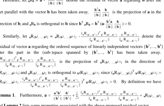
Hereafter, let aRb ≡ a - || || T b a b || || b b

denote the residual of vector a regarding b after the part parallel with the vector b has been taken away.

|| || T b a b || || b b

is the projection of a in the direction of b;and aRb is orthogonal to b since bTaRb = bT

(a-|| || T b a b || || b b ) = 0. Similarly, let aR{b1, …,bk} ≡ aR{b1, …,bk-1} -|| R || R ) R ( } ,..., { } ,..., { T } ,..., { 1 1 1 1 1 1 − − − k k k k k b b b b b b b b a || R || R } ,..., { } ,..., { 1 1 1 1 − − k k k k b b b b b b denote the residual of vector a regarding the ordered sequence of linearly independent vectors {b1,…, bk}

after the part in the (sub-)space spanned by {b1,…, bk} has been taken away.

|| R || R ) R ( } ,..., { } ,..., { T } ,..., { 1 1 1 1 1 1 − − − k k k k k b b b b b b b b a || R || R } ,..., { } ,..., { 1 1 1 1 − − k k k k b b b b b b

is the projection of aR{b1, …,bk-1} in the direction of

bkR{b1, …,bk-1};and aR{b1, …,bk} is orthogonal to bkR{b1, …,bk-1} since (aR{b1, …,bk})T bkR{b1, …,bk-1} =

(aR{b1, …,bk-1} -|| R || R ) R ( } ,..., { } ,..., { T } ,..., { 1 1 1 1 1 1 − − − k k k k k b b b b b b b b a || R || R } ,..., { } ,..., { 1 1 1 1 − − k k k k b b b b b b )T bkR{b1, …,bk-1} = 0. By definition we have Lemma 1. Furthermore, a = || || 1 1 T b b a || || 1 1 b b + k j 2Σ= _|| _R _|| R ) R ( } ,..., { } ,..., { T } ,..., { 1 1 1 1 1 1 − − − j j j j j b b b b b b b b a || R || R } ,..., { } ,..., { 1 1 1 1 − − j j j j b b b b b b + aR{b1,…,bk}

and Lemma 2 lists some properties associated with the above proposed residual vector.

Lemma 1: If a is linearly dependent with b, then aRb = 0. Similarly, if a can be linearly

represented by the set of vectors {b1,…, bk},3 then aR{b1, …,bk} = 0.

Lemma 2: (i) aRb is orthogonal to b. (ii) aR{b1, …,bk} is orthogonal to the subspace spanned

by the set of linearly independent vectors {b1,…, bk}. (iii) If aR{b1, …,bk} = 0, then

aR{b1, …,bk+1} = 0.

3. The Proposed Construction Procedure

Table 1 presents the proposed procedure for constructing a correlated SLFN appropriate for fitting the mapping embedded in {(x1, t1), …, (xN, tN)}.

Table 1. The proposed deterministic procedure for constructing an appropriate correlated SLFN for the mapping requirement of {(x1, t1), …, (xN, tN)}. T ≡ (t1, t2, …, tN)T and v(w0,w)

≡ (a1

(w0,w), a2(w0,w), …, aN(w0,w))T is a N × 1 vector with the cth component being ac(w0,w)

≡ tanh(wT

xc + w0), in which w ≡ (w1, w2, …, wm)T.

Step 1: Calculate TR1. If TR1 = 0, then (i) claim that the fitting job requests no hidden

node; (ii) set the bias of output node as

1 1 1 T T T

and the weight vector between the output

(5)

node and the input layer as 0; and (iii) stop.

Step 2: Apply the C-step to all N observations to obtain the m+1 input samples that are linearly independent. Let I(m+1) be the set of indices of these samples and I(N) be the set of indices of all samples.

Step 3: Calculate c

t

~ _{which equates tanh}-1

( 2 min max 1 min ) ( ) ( ) ( + − + − ∈ ∈ ∈ c N c c N c c N c c t t t t I I I ) from {tc: ∀ c ∈ I(m+1)}. Next, apply the linear regression method to the data set {(xc, _t~c): ∀ c ∈ I(m+1)} to get a set of m+1 weights.

Step 4: Set one hidden node in the network whose values of 2 10

w and 2

1

w are assigned

as the values of the weights obtained in Step 3, and initial values of 3 0 w and 3 1 w are assigned as min 1 ) ( − ∈ c N

c I t and max( ) min( ) 2

+ − ∈ ∈ c N c c N

c I t I t , respectively. Then set γ1 = 1 and p =

1. Step 5: If 3 0 w 1 + p j 1= Σ 3 j w v( 2 0 j w , 2 j

w ) = T, then (i) claim that the fitting job requests p hidden nodes with the bias and weights being the above 3

0 w , 2 0 j w , 2 j w , and 3 j w for all 1 ≤ j ≤ p; and (ii) stop.

Step 6: If 3 0 w 1 + p j 1= Σ 3 j w v( 2 0 j w , 2 j w ) ≠ T, then solve γ , 0 min w ||T {, ( , ), , ( , ), ( 0, 12)} 2 2 0 2 1 2 10 R₁_v_w _w _v_w _w _v_w _γ_w p p K || 2 and let ( * 0 w ,γ*) ≡ arg( γ , 0 min w ||T {, ( , ), , ( , ), ( , )} 2 1 0 2 2 0 2 1 2 10 R₁_v_w _w _v_w _w _v_w _γ_w p p K || 2 ). Step 7: set γp+1 = γ*, w2p+1,0= * 0 w , 2 1 + p w = γp+1w12, and p +1 Æ p.

Step 8: Apply the linear regression method to the data set {((ac( 2 10 w , 2 1 w ), ac(w202 , 2 2 w ), …, ac( 2 0 p w , 2 p

w ))T, tc): ∀ c ∈ I(N)} to get values of 3 0

w and 3

j

w , ∀ j = 1, …, p. Then go to Step 5.

Step 2 releases m+1 linearly independent input samples through applying the C-step to all N input samples.4 Let I(m+1) be the set of indices of these (linearly independent) input samples. Step 3 calculates c

t ~ via tanh-1( 2 min max 1 min ) ( ) ( ) ( + − + − ∈ ∈ ∈ c N c c N c c N c c t t t t I I

I ) ∀ c ∈ I(m+1). Then Step 3

applies the linear regression method to the data set {(xc, c t

~

): ∀ c ∈ I(m+1)} to get the unique solution of ( 2

10 w , 2

1

w ) of system (6), which is a system of m+1 linear equations in m+1 unknowns.

(6)

2 10 w + m j 1= ∑ 2 1 j w xcj = c t ~ _{∀ c ∈ I(m+1). (6)}

Step 4 sets up the network with one hidden node whose values of ( 2 10 w , 2

1

w ) are assigned as obtained in Step 3. The initial values of 3

0

w and 3

1

w are assigned as min 1

) ( − ∈ c N c I t and 2 min max ) ( ) ( − ∈ + ∈ c N c c N

c I t I t , respectively. According to Rousseeuw and Van Driessen (2002), this

setup network renders ce2 = 0 ∀ c ∈ I(m+1) and is a good approximation of the LTS estimator.

Step 5 denotes the stopping criterion of the proposed procedure.

The minimization in Step 6 and the assignment in Step 7 determine the bias and weights for the connections of the input nodes to the most newly recruited hidden node. All biases and weights for the connections of the input nodes to the previously recruited hidden nodes are unchanged. Furthermore, the assignment of Step 7 renders the constructed SLFN correlated since 2

j

w = γjw12, j =1, …, p.

4. The Correctness of the Proposed Procedure

We now prove that the correlated SLFN constructed by the procedure stated in Table 1 meets the mapping requirement of {(x1, t1), …, (xN, tN)} without error.

Tsaih and Wan (2007) state that, for any given {(xc, tc): ∀ c = 1, …, N}, there exists a set

of {( 2

0

j

w ,γjw12), j =1, …, N-1} such that the associated square matrix (1, v( 2 10 w , 2 1 w ), …, v( 2 0 , 1 − N

w ,γN-1w12)) is invertible and the mapping requirement is achieved perfectly. Therefore,

we have Lemma 3 and the proposed procedure will stop at any p with 0 ≤ p ≤ N-1. Lemma 3: If p < N-1, then there always exist w0 and γ such that ( , ) {, ( , ), , ( 2 , 2)}

0 2 1 2 10 2 1 0 R w wp p w w 1v w v w v γ K ≠ 0.

Proof of Lemma 3: Suppose there is a p < N-1 such that there are no w0 and γ to render

)} , ( , ), , ( , { ) , ( 2 2 0 2 1 2 10 2 1 0 R w wp p w w 1v w v w

v γ K ≠ 0. In other words, p < N-1 and there are no w0 and γ such that v(w0,

γ 2 1

w ) is linearly independent with {1, v( 2

10 w , 2 1 w ), v( 2 20 w , 2 2 w ), …, v( 2 0 p w , 2 p w )}. This

contradicts with the statement of Tsaih and Wan (2007). Q.E.D.

When the procedure stops at Step 1, the SLFN constructed at Step 1 meets the mapping requirement of {(x1, t1), …, (xN, tN)} without error since TR1 = 0. On the other hand, it is

obvious to have Lemma 4, which states the necessary condition of a SLFN with p hidden nodes appropriate for the mapping requirement of {(x1, t1), …, (xN, tN)}. Thus the stopping criterion stated in Step 5 is suitable.

Lemma 4: Regarding the mapping samples of {(x1, t1), …, (xN, tN)}, the SLFN with p hidden nodes is appropriate for the mapping requirement if 3

0 w 1 + p j 1= Σ 3 j w v( 2 0 j w , 2 j w ) = T.

Consider the case of 3

0 w 1 + 1 1 − = Σ p j 3 j w v( 2 0 j w , 2 j w ) ≠ T and 3 0 w 1 + p j 1= Σ 3 j w v( 2 0 j w , 2 j w ) = T. Namely, _{_,₍ _, _), _, ₍ 2_, 2_)} 0 2 1 2 10 R j j w w w v w v 1

T _K ≠ 0 for each 1 ≤ j ≤ p-1 and {, ( , ), , ( 2, 2)}

0 2 1 2 10 R p p w w w v w v 1 T _K = 0. For each 1

≤ j ≤ p-1, from calculation, we have _{_, ₍ _, _), _, ₍ _, _), ₍ _, 2_)} 1 0 2 2 0 2 1 2 10 R₁_v _w _v _w _v _w T w K wj j w _γ = {, ( , ), , ( , )} 2 2 0 2 1 2 10 R j j w w w v w v 1 T _K -|| R || R ) R ( )} , ( , ), , ( , { ) , ( )} , ( , ), , ( , { ) , ( T )} , ( , ), , ( , { 2 2 0 2 1 2 10 2 1 0 2 2 0 2 1 2 10 2 1 0 2 2 0 2 1 2 10 j j j j j j w w w w w w w w w v w v 1 w v w v w v 1 w v w v w v 1 T K K K γ γ || R || R )} , ( , ), , ( , { ) , ( )} , ( , ), , ( , { ) , ( 2 2 0 2 1 2 10 2 1 0 2 2 0 2 1 2 10 2 1 0 j j j j w w w w w w w v w v 1 w v w v w v 1 w v K K γ γ and

(7)

|| _{_, ₍ _, _), _, ₍ _, _), ₍ _, 2_)} 1 0 2 2 0 2 1 2 10 R₁_v _w _v _w _v _w T w K wj j w γ || 2 = || _{_, ₍ _, _), _, ₍ 2_, 2_)} 0 2 1 2 10 R j j w w w v w v 1 T _K || 2 (1-( || R || ) R ( )} , ( , ), , ( , { T )} , ( , ), , ( , { 2 2 0 2 1 2 10 2 2 0 2 1 2 10 j j j j w w w w w v w v 1 T w v w v 1 T K K || R || R )} , ( , ), , ( , { ) , ( )} , ( , ), , ( , { ) , ( 2 2 0 2 1 2 10 2 1 0 2 2 0 2 1 2 10 2 1 0 j j j j w w w w w w w v w v 1 w v w v w v 1 w v K K γ γ

)2). Hence we have Lemma 5. Furthermore, suppose

)} , ( , ), , ( , { 2 2 0 2 1 2 10 R p p w w w v w v 1 T _K ≠ 0, || {, ( , ), , ( , ), ( , 2)} 1 * * 0 2 2 0 2 1 2 10 R₁_v _w _v _w _v _w T w K wp p wγ || 2 = 0 if and only if ( || R || ) R ( )} , ( , ), , ( , { T )} , ( , ), , ( , { 2 2 0 2 1 2 10 2 2 0 2 1 2 10 p p p p w w w w w v w v 1 T w v w v 1 T K K || R || R )} , ( , ), , ( , { ) , ( )} , ( , ), , ( , { ) , ( 2 2 0 2 1 2 10 2 1 * * 0 2 2 0 2 1 2 10 2 1 * * 0 p p p p w w w w w w w v w v 1 w v w v w v 1 w v K K γ γ

)2 = 1, which implies the following Lemma 6 is true.

Lemma 5: If _{_, ₍ _, _), _, ₍ 2_, 2_)} 0 2 1 2 10 R j j w w w v w v 1 T _K ≠ 0, then _γ , 0 min w || {, ( , ), , ( , ), ( 0, 21)} 2 2 0 2 1 2 10 R w v w v w v 1 T w K wj j wγ || 2 > || _{_, ₍ _, _), _, ₍ 2_, 2_)} 0 2 1 2 10 R j j w w w v w v 1 T _K || 2 .

Proof of Lemma 5: From Lemma 3, there always exists w0 and γ such that

)} , ( , ), , ( , { ) , ( 2 2 0 2 1 2 10 2 1 0 R j j w w w w 1v w v w

v γ K is a non-zero vector. Now {, ( , ), , ( , ), ( , 2)}

1 0 2 2 0 2 1 2 10 R w v w v w v 1 T w K wj j w γ = )} , ( , ), , ( , { 2 2 0 2 1 2 10 R j j w w w v w v 1 T _K -|| R || R ) R ( )} , ( , ), , ( , { ) , ( )} , ( , ), , ( , { ) , ( T )} , ( , ), , ( , { 2 2 0 2 1 2 10 2 1 0 2 2 0 2 1 2 10 2 1 0 2 2 0 2 1 2 10 j j j j j j w w w w w w w w w v w v 1 w v w v w v 1 w v w v w v 1 T K K K γ γ || R || R )} , ( , ), , ( , { ) , ( )} , ( , ), , ( , { ) , ( 2 2 0 2 1 2 10 2 1 0 2 2 0 2 1 2 10 2 1 0 j j j j w w w w w w w v w v 1 w v w v w v 1 w v K K γ γ and )} , ( , ), , ( , { ) , ( 2 2 0 2 1 2 10 2 1 0 R w wj j w w 1v w v w v γ K and {, ( , ), , ( , ), ( , 2)} 1 0 2 2 0 2 1 2 10 R₁_v _w _v _w _v _w

T w K wj j w γ are orthogonal to each other. Thus,

|| _{_, ₍ _, _), _, ₍ 2_, 2_)} 0 2 1 2 10 R j j w w w v w v 1 T _K || 2 > || _{_, ₍ _, _), _, ₍ _, _), ₍ _, 2_)} 1 0 2 2 0 2 1 2 10 R w v w v w v 1 T w K wj j w γ || 2

. In other words, the optimization of

γ , 0 min w || {, ( , ), , ( , ),( , )} 2 1 0 2 2 0 2 1 2 10 R₁_v _w _v _w _v _w T w K wj j w γ || 2 leads to a non-zero ₍ _, ₎ _{_, ₍ _, _), _, ₍ 2_, 2_)} 0 2 1 2 10 2 1 * * 0 R j j w w w w 1v w v w v γ K , in which ( * 0 w ,γ*) ≡ arg( γ , 0 min w || {, ( , ), , ( , ), ( 0, 12)} 2 2 0 2 1 2 10 R₁_v _w _v _w _v _w T w K wj j w γ || 2 ) and || _{_, ₍ _, _), _, ₍ _, _), ₍ _,_* 2_)} 1 * 0 2 2 0 2 1 2 10 R₁_v _w _v _w _v _w T w K wj j w γ || 2 < || _{_, ₍ _, _), _, ₍ 2_, 2_)} 0 2 1 2 10 R j j w w w v w v 1 T _K || 2 . Q.E.D. Lemma 6: Suppose || _{_, ₍ _, _), _, ₍ 2_, 2_)} 0 2 1 2 10 R p p w w w v w v 1 T _K || 2_{≠ 0. ||} )} , ( ), , ( , ), , ( , { 2 1 * * 0 2 2 0 2 1 2 10 R₁_v _w _v _w _v _w T w K wp p w γ || 2 = 0 if and only if )} , ( , ), , ( , { 2 2 0 2 1 2 10 R p p w w w v w v 1 T _K and ( , ) {, ( , ), , ( 2, 2)} 0 2 1 2 10 2 1 * * 0 R w wp p w w 1v w v w v γ K are parallel.

Lemma 7: The (sub-)space spanned by the set of linearly independent vectors {b1,…, bk} is equivalent with the one spanned by the set of orthonormal vectors { || || 1 1 b b , || R || R 1 2 1 2 b b b b _,…, || R || R } ,..., { } ,..., { 1 1 1 1 − − k k k k b b b b b b }.

Proof of Lemma 7: Let us prove by induction. It is trivial for the case of any set of two linearly independent vectors {b1, b2} since b2Rb1 is orthogonal to b1 and b1Rb2 is orthogonal

to b2.

Now consider the case of any set of k+1 linearly independent vectors {b1,…, bk+1} with k ≥ 2. Assume the subspace spanned by the subset of vectors {b1

,…, bk} is equivalent with the one spanned by the set of orthonormal vectors {

|| || 1 1 b b , || R || R 1 2 1 2 b b b b _{, …,} || R || R } ,..., { } ,..., { 1 1 1 1 − − k k k k b b b b b b }. The

(8)

vector bk+1 can be represented as || || ) ( 1 1 T 1 b b bk+ || || 1 1 b b + k j 2Σ= _|| _R _|| R ) R ( } ,..., { } ,..., { T } ,..., { 1 1 1 1 1 1 1 − − − + j j j j j k b b b b b b b b b || R || R } ,..., { } ,..., { 1 1 1 1 − − j j j j b b b b b b +

bk+1R{b1, …,bk}, in which bk+1R{b1, …,bk} is a non-zero vector since bk+1 is linearly independent

with the set of vectors {b1,…, bk}. Thus the (sub-)space spanned by the set of vectors {b1,…, bk+1} is equivalent with the one spanned by the set of vectors {

|| || 1 1 b b , || R || R 1 2 1 2 b b b b _,…, bk+1R{b1, …,bk}}. Furthermore, (bk+1R{b1, …,bk})T b1 = (bk+1R{b1, …,bk-1} -|| R || R ) R ( } ,..., { } ,..., { T } ,..., { 1 1 1 1 1 1 1 − − − + k k k k k k b b b b b b b b b || R || R } ,..., { } ,..., { 1 1 1 1 − − k k k k b b b b b b

)T b1 = 0; and, for any 2 ≤ j ≤ k-1, (bk+1R{b1, …,bk})TbjR{b1, …,bj-1} = (bk+1R{b1, …,bk-1}

-|| R || R ) R ( } ,..., { } ,..., { T } ,..., { 1 1 1 1 1 1 1 − − − + k k k k k k b b b b b b b b b || R || R } ,..., { } ,..., { 1 1 1 1 − − k k k k b b b b b b )T bjR{b1, …,bj-1} = 0; and (bk+1R{b1, …,bk})T bkR{b1, …,bk-1} = (bk+1R{b1, …,bk-1} -|| R || R ) R ( } ,..., { } ,..., { T } ,..., { 1 1 1 1 1 1 1 − − − + k k k k k k b b b b b b b b b || R || R } ,..., { } ,..., { 1 1 1 1 − − k k k k b b b b b b )TbkR{b1, …,bk-1} = 0. Q.E.D. Let u0 ≡ || || 1 1 , u1 ≡ || R || R ) , ( ) , ( 2 1 2 10 2 1 2 10 1 w v 1 w v w w , and uj ≡ || R || R )} , ( , ), , ( , { ) , ( )} , ( , ), , ( , { ) , ( 2 1 2 0 , 1 2 1 2 10 2 2 0 2 1 2 0 , 1 2 1 2 10 2 2 0 − − − − j j j j j j j j w w w w w w w v w v 1 w v w v w v 1 w v K K _{for all 2 ≤ j ≤ p.} Thus TT uk = ( 3 0 w 1 + p j 1Σ= 3 j w v( 2 0 j w , 2 j w ))T uk = p k jΣ= 3 j w (v( 2 0 j w , 2 j

w ))T uk for all 1 ≤ k ≤ p, since, from

Lemma 7, v( 2

0

j w , 2

j

w ) is in the subspace spanned by {u0, u1,…, uj} and (uj)T uk ≠ 0 ∀ k ≤ j ≤ p.

Thus 3 p w ≡ _p p p p w w u v u T T 2 2 0 T )) , ( ( , 3 j w ≡ j j j j p j l l l l w w w u w v u w v T T 2 2 0 T 1 2 2 0 3 )) , ( ( ) ) , ( ( − ∑ + =

for all p-1 ≥ j ≥ 1, and 3 0 w ≡ 0 T 0 T 1 2 2 0 3 ) ) , ( ( u 1 u w v T−∑ = p l l l l w w .

Let A-1≡ I and Ak≡ Ak-1 - uk(uk)T for all 0 ≤ k ≤ N-1. Thus, Ak= I - k j 0Σ= u

j

(uj)T for all 0 ≤

k ≤ N-1. Since all vectors in the set {u0, u1,…, uk} are orthonormal, (Ak)T = Ak and Ak Ak = Ak. Furthermore, because TR{u0,u1,…,up} = T

-p j 0Σ= (u

j

)T T uj, TR{u0,u1,…,up} = Ap T. Similarly,

v(w0,w)R{u0,u1,…,up} = Ap v(w0,w). Thus, _v(w0,w)R{u0,u1,…,up}T T = v(w0,w)T Ap T, v(w0,w)T

TR{u0,u1,…,up} = v(w0,w)T Ap T, _v(w0,w)R{u0,u1,…,up}TTR{u0,u1,…,up} = v(w0,w)T Ap T, TR{u0,u1,…,up}T

TR{u0,u1,…,up} = TT Ap T, and ||_v(w0,w)R{u0,u1,…,up}||2 = v(w0,w)T Ap v(w0,w). thus, ||TR_v(w0,w)||2 =

TT T -) , ( ) , ( ) ) , ( ( 0 T 0 2 T 0 w v w v T w v w w w and ||TR_{{u0,u1,…,up,v(w0,w)}}||2 = TT Ap T -) , ( ) , ( ) ) , ( ( 0 T 0 2 T 0 w v A w v T A w v w w w p p = ) , ( ) , ( ) ) , ( ( ) , ( ) , ( 0 T 0 2 T 0 0 T 0 T w v A w v T A w v w v A w Tv A T w w w w w p p p p ₋ . Lemma 8: If _{_, ₍ _, _), _, ₍ 2_, 2_)} 0 2 1 2 10 R p p w w w v w v 1

T _K ≠ 0 and there exists a vector v(w0,

2 1 w r ) such that )} , ( ), , ( , ), , ( , { 2 1 0 2 2 0 2 1 2 10 R₁_v _w _v _w _v _w T w K wp p w γ = 0, then 0,γ min w || {,( , ), , ( , ),( 0, 12)} 2 2 0 2 1 2 10 R₁_v _w _v _w _v _w T w K wp p w γ || 2 leads to a non-zero

(9)

)} , ( , ), , ( , { ) , ( 2 2 0 2 1 2 10 2 1 * * 0 R w wp p w w 1v w v w v γ K such that _|| _R _|| R )} , ( , ), , ( , { ) * , ( )} , ( , ), , ( , { ) * , ( 2 2 0 2 1 2 10 2 1 * 0 2 2 0 2 1 2 10 2 1 * 0 p p p p w w w w w w w v w v 1 w v w v w v 1 w v K K γ γ and || R || R )} , ( , ), , ( , { ) , ( )} , ( , ), , ( , { ) , ( 2 2 0 2 1 2 10 2 1 0 2 2 0 2 1 2 10 2 1 0 p p p p w w w w w w w v w v 1 w v w v w v 1 w v K K γ γ

are parallel and || _{_, ₍ _, _), _, ₍ _, _), ₍ _,_* 2_)} 1 * 0 2 2 0 2 1 2 10 R₁_v _w _v _w _v _w T w K wp p w_γ || 2 = 0. Proof: Let p+1 u ≡ || R || R } , , { ) , ( } , , { ) , ( 1 0 1 0 p p w w u u w v u u w v K K _{. Thus, facts of} )} , ( , ), , ( , { 2 2 0 2 1 2 10 R p p w w w v w v 1 T _K ≠ 0 and )} , ( ), , ( , ), , ( , { 2 1 0 2 2 0 2 1 2 10 R₁_v _w _v _w _v _w T w K wp p w _γ = 0 imply that {u 0 , u1, …, up, p+1 u } is an orthonormal set, T = p j 0Σ= (u j )T T uj + ( p+1 u )T T p+1 u , and ( p+1 u )T T ≠ 0. Suppose v(w0,γw12) ≡ p j 0Σ= (u j )T v(w0,γw12) u j + ( p+1 u )T v(w0,γw12) 1 + p u +_v( _, 2₎ _{ 0_,1_,..., _, 1_} 1 0 R + p p wγw u u u u . Thus, || _{ _, _,_, _, _,₍ _, 2_)} 1 0 1 0 R_u _u _u _v _w T p w _γ K || 2 = ) , ( )) , ( ( ) )) , ( (( ) , ( )) , ( ( 2 1 0 T 2 1 0 2 T 2 1 0 2 1 0 T 2 1 0 T w v A w v T A w v w v A w v T A T γ γ γ γ γ w w w w w p p p p ₋ = ) , ( )) , ( ( 1 2 1 0 T 2 1 0 w A v w v w γ p w γ [(T T p+1 u )2 (v(w0,γw12)) T (( p+1 u )T v(w0,γw12) 1 + p u + _v( _, 2₎ _{0_,1_,..., _, 1_} 1 0 R p p+ w γw u u u u ) - (( p+1 u )T T ( p+1 u )T v(w0,γw12)) 2 ] = ) , ( )) , ( ( ) ( 2 1 0 T 2 1 0 2 1 T w v A w v u T γ γ w w p p+ [((( p+1 u )T v(w0,γw12)) 2 + ||_v( _, 2₎ _{ 0_,1_,..., _, 1_} 1 0 R p p+ wγw u u u u || 2 ) - (( p+1 u )T v(w0,γw12)) 2 ] = ) , ( )) , ( ( ) ( 2 1 0 T 2 1 0 2 1 T w v A w v u T γ γ w w p p+ ||_v( _, 2₎ _{ 0_,1_,..., _, 1_} 1 0 R p p+ w γw u u u u || 2 . If ||_v( _, 2₎ _{ 0_,1_,..., _, 1_} 1 0 R + p p w γw u u u u || 2 > 0, then || _{ _, _,_, _, _,₍ _, 2_)} 1 0 1 0 R _u _u _u _v _w T p w _γ K || 2 > _{ _, _,..., _,_v( _, _)} 2 0 1 0 R_u _u _u _w T p w because of a non-zero ( p+1

u )T T. Therefore, the optimization of

γ , 0 min w || {, ( , ), , ( , ), ( 0, 12)} 2 2 0 2 1 2 10 R₁_v _w _v _w _v _w T w K wp p w γ || 2 leads to a non-zero ₍ _, ₎ _{_, ₍ _, _), _, ₍ 2 _, 2_)} 0 2 1 2 10 2 1 * * 0 R w wp p w w 1v w v w v γ K such that ||v( ,* 2) { 0,1,..., , 1} 1 * 0 R + p p wγ w u u u u || 2 = 0. From Lemma 6, || R || R } , , , { ) * , ( } , , , { ) * , ( 1 0 2 1 * 0 1 0 2 1 * 0 p p w w u u u w v u u u w v K K γ γ and || R || R } , , , { ) , ( } , , , { ) , ( 1 0 0 1 0 0 p p w w u u u w v u u u w v K

K _{are parallel and thus, ||}

)} * , ( ), , ( , ), , ( , { 2 1 * 0 2 2 0 2 1 2 10 R₁_v _w _v _w _v _w T w K wp p w γ || 2 = 0. Q.E.D. References

1. M. Me’zard and J. Nadal, Learning in feedforward layered networks: The tiling algorithm.

Journal of Physics. A 22, 2191‒ 2204 (1989).

2. S. Fahlman and C. Lebiere, The Cascade-Correlation Learning Architecture. In

Touretzky, D. (Eds.), Advances in Neural Information Processing Systems II (Denver, 1989) Morgan Kaufmann, San Mateo (1990).

3. M. Frean, The Upstart Algorithm: A Method for Constructing and Training Feedforward

Neural Networks. Neural Computation. 2, 198‒ 209(1990).

4. G. Huang and H. Babri, Upper bounds on the number of hidden neurons in feedforward

networks with arbitrary bounded nonlinear activation functions. IEEE Transactions on Neural Networks. 9, 224‒ 229(1998).

5. D. Rumelhart, G. Hinton, and R. Williams, “Modeling Internal Representations By Error Propagation,” in Parallel Distributed Processing: Explorations in the Microstructure of

(10)

Cognition, vol. 1, D. Rumelhart and J. McClelland, Eds. Cambridge, MA: MIT Press,

1986, pp. 318-362.

6. P. J. Rousseeuw and A. M. Leroy, Robust Regression and Outlier Detection. New York: Wiley, 1987.

7. R. D. Cook and S. Weisberg, Residuals and Influence in Regression, London: Chapman and Hall, 1982.

8. A. C. Atkinson, Plots, Transformations and Regression, Oxford: Oxford University Press, 1985.

9. F. R. Hampel, E. M. Ronchetti, P. J. Rousseeuw and W. A. Stahel, Robust Statistics: The

Approach Based on Influence Functions. New York: John Wiley, 1986.

10. A. Zaman, P. J. Rousseeuw and M. Orhan, “Econometric Applications of High-Breakdown Robust Regression Techniques,” Econometrics Letters, vol. 71, pp. 1-8, Apr. 2001.

11. A. C. Atkinson and T. C. Cheng, “Computing Least Trimmed Squares Regression with the Forward Search,” Statistics and Computing, vol. 9, pp. 251-263, Nov. 1999.

12. A. C. Atkinson, “Fast Very Robust Methods for the Detection of Multiple Outliers,”

Journal of the American Statistical Association, vol. 89, pp. 1329-1339, 1994.

13. P. J. Rousseeuw and K. Van Driessen, “Computing LTS Regression for Large Data Sets,” Estadistica, vol. 54, 163-190, 2002.

14. A. J. Stromberg, “Computation of High Breakdown Nonlinear Regression Parameters,” Journal of the American Statistical Association, vol. 88, pp. 237-244, Mar. 1993.

計畫成果自評：

(11)

出席國際學術會議心得報告

計畫編號 95-2416-H-004-049 計畫名稱相關性隱藏節點與學習演算法出國人員姓名服務機關及職稱蔡瑞煌國立政治大學資訊管理學系,教授會議時間地點 July 18-24, 2007, Salt Lake City, U.S.A.

會議名稱 Joint Conference on Information Sciences

發表論文題目 A Constructive Learning Procedure 一、參加會議經過

我於 7/19 晚上到達 Salt Lake City。我於 7/20 主持 section CIEF-III 並於其間發表論文。附件一是相關議程。

我也於 7/20~7/21 聆聽此次會議裡的 Keynote Speeches 和論文發表。

二、與會心得

(12)

A Constructive Learning Procedure

∗

RAY TSAIH

Department of Management Information Systems, National Chengchi University, No.64, Sec. 2, Jhihnan Rd., Wunshan District,Taipei City 116, Taiwan

This study explores a deterministic learning procedure for the realization of a real-valued single-hidden layer feed-forward neural network (SLFN) with tanh activation functions of the hidden-layer nodes for arbitrary mapping problems.

1. The Constructive Learning Procedure

The proposed learning procedure will use none hidden node initially and recruit (add) more hidden nodes during the learning process. The goal of the proposed constructive learning procedure is to create a SLFN for fitting perfectly all given mapping samples. In the literature, there are some similar procedures; for instance, the tiling algorithm for binary-valued layered feed-forward neural networks (cf. [1]), the cascade-correlation algorithm (cf. [2]), and the upstart algorithm for binary-valued layered feed-forward neural networks (cf. [3]). In contrast to these researches, this study copes with the real-valued SLFN.

2. The Mapping Requirement and Notations

An SLFN provides a nonlinear mapping between x and y, whose form is y = f(x). f is a nonlinear function whose parameters (i.e., weights and biases) are derived from a given data set of mapping samples {(x1, t1),…, (xN, tN)} with xc1 ≠ xc2_{, c}

1 ≠ c2, and with tc the target value of y corresponding to xc. x ≡ (x1, x2,…, xm)T ∈ Rm where xj is the jth input

component, with j from 1 to m.

Hereafter, m and p denote the numbers of adopted input and hidden nodes, repsectively; w2j0 stands for the bias of

the jth hidden node; 2

j w ≡ ( 2 1 j w , 2 2 j w ,…, 2 jm

w )T for the weights between the jth hidden node and input layer; 3 0

w for the bias of the output node; and w3≡ (w13,

3 2

w ,…,w3p)

T

for the weights between the output node and all hidden nodes. Characters in bold represent column vectors; the superscript T indicates transposition.

Let the tanh(t) activation function be used by all hidden nodes and a linear activation function be used by the output node. Thus, given the cth sample xc, the activation value of the jth hidden node ac( 2

0

j

w , 2

j

w ) and the output value yc are as follows: ac(w2j0, 2 j w ) ≡ tanh( 2 0 j w + m i 1= ∑ 2 ji w x_ic); (1) yc ≡ 3 0 w + p j 1Σ= 3 j w ac( 2 0 j w , 2 j w ). (2)

Given the N mapping samples, let v( 2 0 j w , 2 j w ) ≡ (a1( 2 0 j w , 2 j w ), a2( 2 0 j w , 2 j w ),…, aN( 2 0 j w , 2 j w ))T ∈

(-1,1)N be the responding vector of the jth hidden node with the cth component being ac( 2 0

j

w , 2

j

w ).

Furthermore, let 1 be a N × 1 vector with all components 1 and T ≡ (t1

, t2, …, tN)T∈ RN. Thus, the set of simultaneous equations 3

0 w + p j 1Σ= 3 j w tanh( 2 0 j w +m i 1= ∑ 2 ji w xic) = t c_{∀ c = 1, …, N is equivalent to}

system (3), which states that T is in the (sub-)space spanned by 1 and p responding vectors,

∗_{This study is supported by National Science Council of R.O.C. under Grants No. NSC 92-2416-H-004-004, NSC 93-2416-H-004-015, and NSC}

(13)

{v( 2 0 j w , 2 j w ), j = 1, …, p}. 3 0 w 1 + p j 1= Σ 3 j w v(w2_j₀,w2j) = T. (3) Hereafter, aRb ≡ a-|| || T b a b || || b b

denotes the residual of vector a regarding b after the part parallel with the vector b has been taken away. Furthermore, aR{b1,…,bk} ≡ aR{b1,…,bk-1}

-|| R || R } ,..., { } ,..., { T 1 1 1 1 − − k k k k b b b b b b a || R || R } ,..., { } ,..., { 1 1 1 1 − − k k k k b b b b b b

denotes the residual of vector a regarding the ordered sequence of vectors {b1,…, bk} after the parts parallel with vectors bjs have been taken away.

Note that aR{b1, …,bk} = a-|| || 1 1 T b b a || || 1 1 b b - k j 2Σ= _|| _R _|| R } ,..., { } ,..., { T 1 1 1 1 − − j j j j b b b b b b a || R || R } ,..., , { } ,..., , { 1 1 0 1 1 0 − − j j j j b b b b b b b b and thus a = || || 1 1 T b b a || || 1 1 b b + k jΣ=2 _|| _R _|| R } ,..., { } ,..., { T 1 1 1 1 − − j j j j b b b b b b a || R || R } ,..., , { } ,..., , { 1 1 0 1 1 0 − − j j j j b b b b b b b b

+ aR{b1, …,bk}. Furthermore, we have Lemma 1 below, which

lists some properties associated with the above proposed residual vector.

Lemma 1: (i) If a is linearly dependent with b, then aRb = 0. Similarly, if a can be linearly represented by the set of

vectors {b1,…, bk},1 then aR{b1, …,bk} = 0. (ii) aRb is orthogonal to b. Similarly, aR{b1, …,bk} is orthogonal to all vectors in

the set {b1,…, bk}. (iii) If aR{b1, …,bk} = 0, then aR{b1, …,bk+1} = 0.

3. The Proposed Constructive Procedure

Table 1 presents the proposed procedure for constructing a SLFN appropriate for fitting the mapping embedded in {(x1,

t1), …, (xN, tN)}.

Table 1. The proposed deterministic procedure for constructing an appropriate SLFN for the mapping requirement of {(x1_{, t}1_{), …, (x}N_{, t}N_{)}. T ≡ (t}1_,

t2_{, …, t}N₎T_{and v(w}

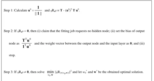
0,w) ≡ (a1(w0,w), a2(w0,w), …, aN(w0,w))T is a N × 1 vector with the cth component being ac(w0,w) ≡ tanh(wT xc + w0), in which w ≡ (w1, w2, …, wm)T. Step 1: Calculate u0₌ || || 1 1 and TRu0 ≡ T - (u0)T T u0.

Step 2: If TRu0 = 0, then (i) claim that the fitting job requests no hidden node; (ii) set the bias of output

node as _T ₀ 0 T u 1 u T

and the weight vector between the output node and the input layer as 0; and (iii)

stop.

Step 3: If TRu0 ≠ 0, then solve

w , 0 min w ||TR{v(w0,w)}|| 2_{and let w}

0* and w* be the obtained optimal solution.

(14)

Then set w₁₀2 = w0*, 2 1 w = w*_{, u}1_≡ || ) , ( || ) , ( 2 1 2 10 2 1 2 10 w v w v w w , and p = 1.

Step 4: Calculate TR{u1,…,up}.

Step 5: If TR{u1,…,up} = 0, then (i) claim that the fitting job requests p hidden nodes with the bias and

weights of the jth hidden node being the above w2j0 and 2 j w , ∀ j = 1, …, p; (ii) set 3 0 w ≡ 0, 3 p w ≡ _p p p p w w u v u T T 2 2 0 T ) , ( , and 3 j w ≡ _j j j j p j l l l l w w w u w v u w v T T 2 2 0 T 1 2 2 0 3 ) , ( ) ) , ( ( ∑ + = −

for all 1 ≤ j ≤ p-1; and

(iii) stop.

Step 6: If TR{u1,…,up} ≠ 0, then calculate u0 =

|| R || R } ..., , { } ..., , { 1 1 p p u u 1 u u 1

and TR{u1,…,up,u0} ≡ TR{u1,…,up} - (u0)T T u0.

Step 7: If TR{u1,…,up,u0} = 0, then (i) claim that the fitting job requests p hidden nodes with the bias and

weights of the jth_{hidden node being the above} 2

0

j

w and w2_j, ∀ j = 1, …, p; (ii) set

3 0 w ≡ _T ₀ 0 T u 1 u T , w3_p≡ _p p p p w w u w v u 1 T T 2 2 0 T 3 0 ) , ( ) ( − , and w3_j≡ _j j j j p j l l l l w w w w u w v u w v 1 T T 2 2 0 T 1 2 2 0 3 3 0 ) , ( ) ) , ( ( ∑ + = − −

for all 1 ≤ j ≤ p-1; and (iii) stop.

Step 8: If TR{u1,…,up,u0} ≠ 0, then solve

w , 0 min w ||TR{u1,…,up,v(w0,w)}|| 2_{and let w}

0* and w* be the obtained optimal

solution. Then (i) set w2_p₊₁_,₀= w0*,

2 1 + p w = w*_{, u}p+1_≡ || R || R } , , { ) , ( } , , { ) , ( 1 2 1 2 0 , 1 1 2 1 2 0 , 1 p p p p p p w w u u w v u u w v K K + + + + , set p +1 Æ p; and (ii) go to Step 4.

4. The Correctness of the Proposed Procedure

We now prove that the procedure stated in Table 1 creates an appropriate SLFN that meets the mapping requirement of {(x1, t1), …, (xN, tN)} without error.

Lemma 2 below is obvious from system (3) and the definition of the residual vector. Lemma 2 states the necessary

condition of a SLFN with p hidden nodes appropriate for the mapping requirement of {(x1, t1), …, (xN, tN)}. Note that,

from Lemma 1 (iii), _{ ₍ _, _),..., ₍ 2 _, 2_)} 0 2 1 2 10 R p p w w w v w v T = 0 results in { ( , ),...,( 2 , 2),} 0 2 1 2 10 R _v _w _v _w ₁

T w w_p _p = 0. Thus the condition stated in Steps 2,

(15)

Lemma 2: Regarding the mapping samples of {(x1

, t1), …, (xN, tN)}, the SLFN with p hidden nodes is appropriate for

the mapping requirement if the associated _{ ₍ _, _),..., ₍ 2_, 2_),_} 0 2 1 2 10 R_v _w _v _w ₁ T w w_p _p equals 0.

Namely, if TRu0 = 0 at Step 2 of Table 1, in which u0 = || || 1 1 , then T = _T ₀ 0 T u 1 u T

and the mapping

requirement asks for no hidden node. Furthermore, because u1 ≡

|| ) , ( || ) , ( 2 1 2 10 2 1 2 10 w v w v w w , uj ≡ || R || R } , , { ) , ( } , , { ) , ( 1 1 2 2 0 1 1 2 2 0 − − j j j j j j w w u u w v u u w v K K

for all j = 2, …, p, and u0 ≡

|| R || R } ..., , { } ..., , { 1 1 p p u u 1 u u 1 , _{ ₍ _, _), _, ₍ 2_, 2_)} 0 2 1 2 10 R p p w w w v w v T _K = TR{u1,…,up} and { ( , ), , ( 2, 2),} 0 2 1 2 10 R_v _w _v _w ₁ T w K w_p _p =

TR{u1,…,up,u0}. Thus, if TR{u1,…,up} = 0 at Step 5 of Table 1, then T =

p j 1= Σ 3 j w v(w2_j₀, 2 j

w ) and the mapping requirement asks for p hidden nodes. If TR{u1,…,up,u0} = 0 at Step 7 of Table 1, then T =w031

+ p j 1= Σ 3 j w v(w2_j₀, 2 j

w ) and the mapping requirement asks for p hidden nodes.

The following Lemmas 3 and 4 show that the proposed procedure will generate a sequence of orthonormal vectors.

Lemma 3: If p < N-1, then there always exist w0 and w such that _{v(w0, w)}R{u1, …,up,u0} ≠ 0.

Proof of Lemma 3: Suppose p < N-1 and there are no w0 and w such that_{v(w0, w)}R{u1, …,up,u0} ≠ 0. In other words, p < N-1

and there are no w0 and w such that v(w0, w) is linearly independent with {u1, …, up, u0}. This contradicts with the

statement of [4] that, for any given {xc ∀ c = 1, …, N}, there exists a set of {(w2j0, 2

j

w ), j =1, …, N-1} such that the associated square matrix (1, v( 2

10 w , 2 1 w ), …, v( 2 0 , 1 − N w , 2 1 − N w )) is invertible. Q.E.D.

Lemma 4: When the proposed procedure stops at some p, 1 ≤ p ≤ N-1, all vectors in the set of {u1

, …, up} or {u1, …, up,

u0

} are orthonormal.

Proof of Lemma 4: It is trivial for the case of p = 1 and {u1

}. As for the case of p = 1 and {u1, u0}, from steps 6 and 7 of Table 1, TRu1 ≠ 0, u0 ≡

|| R || R 1 1 u 1 u 1

, and TR{u1,u0} = 0. Thus u0 is non-zero and, from

Lemma 1 (ii), orthogonal to u1

. Namely, {u1, u0} is an orthonormal set.

Now consider the case of any p with 2 ≤ p ≤ N-1. Then, for each 1 ≤ j ≤ p-1, from Lemma 3, there exists w0 and w such that _v(w0,w)R{u1,…,uj, u0} is not zero and thus, from Lemma 1 (iii),

v(w0,w)R{u1,…,uj} is not zero. Furthermore, as stated in Step 8 of Table 1, TR{u1,…,uj,u0} ≠ 0. Thus

TR{u1,…,uj} ≠ 0, there exists a non-zero _v(w0,w)R{u1,…,uj} that TR{u1,…,uj} = TR_{{u1,…,uj,v(w0,w)}}

+ ₂ } , , { ) , ( } , , { ) , ( T || R || R 1 0 1 0 j j w w u u w v u u w v Τ K K

v(w0,w)R{u1,…,uj}, and, from Lemma 1 (ii), v(w0,w)R{u1,…,uj} and TR_{{u1,…,uj,v(w0,w)}} are

orthogonal to each other. Namely, ||TR{u1,…,uj}||2 ≥ ||TR_{{u1,…,uj,v(w0,w)}}||2. Therefore, the optimization of

w , 0 min w ||TR{u1,…,uj,v(w0,w)}|| 2

leads to a non-zero _{v(w0*, w*)}R{u1,…,uj}, in which (w0*,w*) ≡ arg(

w , 0 min w ||TR{u1,…,uj, v(w0,w)}||2). Thus uj+1 ≡_|| _R _|| R } , , { ) , ( } , , { ) , ( 1 * * 0 1 * * 0 j j w w u u w v u u w v K

K _{is a unit vector and, from Lemma 1 (ii), orthogonal to the set}

(16)

From Steps 6 and 7 of Table 1, if TR{u1,…,up} ≠ 0, u0 = || R || R } ..., , { } ..., , { 1 1 p p u u 1 u u 1

and TR{u1,…,up,u0} = 0, then u0 is non-zero and,

from Lemma 1 (ii), orthogonal to all vectors in the set {u1, …, up}. Namely, {u1, …, up, u0} is an orthonormal set.

Q.E.D. If T = p j=1 Σ 3 j w v(w2_j₀,w2j), then T T_uk = ( p j=1 Σ 3 j w v(w2_j₀,w2j)) T_uk = p k jΣ= 3 j w v(w2_j₀,w2j) T_uk , since v(w2j0, 2 j w ) is in the

subspace spanned by {u1, …, uj} for all j = 1, …, p and (ui)T uj ≠ 0 ∀ i ≠ j. Thus, as stated in Step 5 of Table 1,

3 p w ≡ p p p p w w u v u T T 2 2 0 T ) , ( , 3 j w ≡ j j j j p j l l l l w w w u w v u w v T T 2 2 0 T 1 2 2 0 3 ) , ( ) ) , ( ( ∑ + = −

for all 1 ≤ j ≤ p-1, and 3 0 w ≡ 0. Similarly, if T = 3 0 w 1 + p j=1 Σ 3 j w v(w2_j₀,w2j), then T T_uk = (w031 + p j=1 Σ 3 j w v(w2j0, 2 j w ))T uk = (w301 + p k jΣ= 3 j w v(w2_j₀,w2j)) T_uk . Therefore, as

stated in Step 7 of Table 1, 3 0 w ≡ 0 T 0 T u 1 u T , 3 p w ≡ p p p p w w u w v u 1 T T 2 2 0 T 3 0 ) , ( ) ( − , and 3 j w ≡ j j j j p j l l l l w w w w u w v u w v 1 T T 2 2 0 T 1 2 2 0 3 3 0 ) , ( ) ) , ( ( ∑ + = − − for all 1 ≤ j ≤ p-1. References

1. M. Me’zard and J. Nadal, Learning in feedforward layered networks: The tiling algorithm. Journal of Physics. A

22, 2191‒ 2204(1989).

2. S. Fahlman and C. Lebiere, The Cascade-Correlation Learning Architecture. In Touretzky, D. (Eds.), Advances in

Neural Information Processing Systems II (Denver, 1989) Morgan Kaufmann, San Mateo (1990).

3. M. Frean, The Upstart Algorithm: A Method for Constructing and Training Feedforward Neural Networks. Neural

Computation. 2, 198‒ 209(1990).

4. G. Huang and H. Babri, Upper bounds on the number of hidden neurons in feedforward networks with arbitrary

相關性隱藏節點與學習演算法

行政院國家科學委員會專題研究計畫 成果報告