國
立
交
通
大
學
資訊科學與工程研究所
碩
碩
碩
碩
士
士
士
士
論
論
論
論
文
文
文
文
一個時序工作流程編輯時異常動作的遞增性分
析
An Incremental Anomaly Detection for Temporal Workflow
Specification
研 究 生:吳明勳
指導教授:王豐堅 教授
中
中
中
中
華
華
華
華
民
民
民
民
國
國
國
國
一零三
一零三
一零三
一零三
年
年
年
年
三
三
三
三
月
月
月
月
一個時序工作流程編輯時異常動作的遞增性分析
An Incremental Anomaly Detection for Temporal Workflow
Specification
研 究 生:吳明勳 Student:Ming-Shun Wu
指導教授:王豐堅 Advisor:Feng-Jian Wang
國 立 交 通 大 學
資 訊 科 學 與 工 程 研 究 所
碩 士 論 文
A ThesisSubmitted to Department of Computer and Information Science College of Electrical Engineering and Computer Science
National Chiao Tung University in partial Fulfillment of the Requirements
for the Degree of Master
in
Computer and Information Science March 2014
Hsinchu, Taiwan, Republic of China
一個時序工作流程編輯時異常動作的遞增性分析
學生:吳明勳
指導教授:王豐堅
國立交通大學資訊工程學系﹙研究所﹚碩士班
摘
摘
摘
摘 要
要
要
要
一個好的結構化工作流程是由更小的結構化工作流程和程序所組
成,結構化工作流程裡的控制結構是由平行與選擇結構組成。一個工
作流程可以被轉換成一個結構化工作流程,用來分析 artifact 的異常。
此外,時間因素也被加入到每個程序中,以提高偵測 artifact 異常的準
確度。在這篇論文中,我們首先引進了將一個時序工作流程轉換成一
個時序結構化工作流程的方法,然後在此時序化工作流程上找出異常。
這樣的工作流程被稱之為 TS 工作流程,以及我們也發展出一個批次的
演算法計算異常。由於 CASE 工具的盛行,在工作流程上的遞增性分
析也變得更為重要。然而,在一個時序工作流程裡作遞增式分析並不
容易,因為迴圈及時間的因素使得分析變得更為複雜。我們對編輯工
作流程的動作分類並加以討論,發展出一系列的演算法,這些演算法
是作用在被編輯後的 TS 工作流程上,用來分析有何 artifact 異常產生。
關鍵字
關鍵字
關鍵字
關鍵字: artifact 異常, 遞增性分析, 時間, 工作流程
An Incremental Anomaly Detection for Temporal Workflow Specification
Student:Ming-Shun Wu
Advisors:Dr.
Feng-Jian Wang
Institutes of Computer Science and Engineering
National Chiao Tung University
Abstract
A well-structured workflow is composed of a group of well-structured workflow(s) and process(es), where the control structure is composed of parallel/decision structure. A general workflow can be transformed into a well-structured workflow for the analysis of abnormal artifact behavior. Besides, the temporal factors can be added into each process to help improve the preciseness of anomaly detection. In this thesis, we first introduce how to transform a general workflow with temporal factors into a well-structured one with temporal factors for anomaly detection. The workflow is called a TS workflow, and a batched analysis algorithm is developed. Due to the popularity of CASE tools, the incremental analysis for the workflow is getting important. However, the incremental anomaly detections working in a workflow with temporal factor are difficult, since the loop and related temporal factors introduce complicated problems. We discuss and categorize the edit activities and develop a series of analysis algorithms which are organized in to perform the anomaly detections in the corresponding TS workflow maintained after each edit activity.
致謝
致謝
致謝
致謝
本篇論文的完成,首先要感謝我的指導教授王豐堅博士的指導,使我習得許 多軟體工程上的知識,以及學到撰寫論文的方法與結構,並且學習到有關於遞增 式分析的應用,得到許多的經驗。另外也感謝口試委員吳毅成和廖珗洲老師的建 議與指導,提供寶貴的意見讓我補足論文中不足之處。 其次,感謝實驗室的夥伴們,對我的指導與照顧,使我獲益良多,才得以順 利完成研究。 最後,我要感謝我的家人,因為有你們的支持,讓我心無旁騖地念書,專心 於自己的研究。由衷地感謝各位陪伴我走過這段歲月。Table of Contents
摘要 ... i Abstract ... ii 致謝 ... iii Table of Contents ... iv List of Figures ... v List of Algorithms ... vi Chapter 1 Introduction ... 1Chapter 2 Workflow Definition ... 4
2.1 Definition of a structured workflow ... 4
2.2 A temporal structured workflow ... 6
2.3 Artifact operations and anomalies ... 7
2.4 Loop reduction ... 9
Chapter 3 Temporal Computation for TS Workflow ... 11
3.1 Level Computation for Processes... 11
3.2 Removing Loop(s) in a Workflow ... 16
3.3 Temporal Computation inside a Workflow without Loops ... 21
Chapter 4 Anomaly Detection in a TS Workflow ... 25
4.1 Anomaly Detection in a Batch ... 25
4.2 Incremental anomaly detection ... 31
4.2.1 Detection inside a TS workflow ... 31
4.2.2 Computing concurrent and nonempty set ... 38
4.2.3 Anomaly detection with the algorithms in above two subsections ... 43
4.3 A Summary for our Incremental Analysis ... 50
Chapter 5 Conclusion and Future Work ... 52
List of Figures
Figure 2.1 The graph notation in a workflow ... 4
Figure 2.2 The blocks in a workflow ... 5
Figure 2.3 The method of computing EAI ... 6
Figure 2.4 Artifact states transition diagram ... 8
Figure 2.5 The loop is transformed into an acyclic structure ... 10
Figure 3.1 A sample TS workflow, where each process is associated with EAI ... 11
Figure 3.2 A sample workflow, where each process is associated with level value .... 12
Figure 3.3 The methods of computing branch stack for each type of process ... 14
Figure 3.4 The branch stacks attached on each process in workflow in Figure 3.2 ... 14
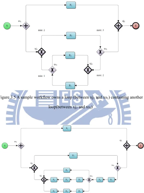
Figure 3.5 A sample workflow owns a loop (between xj1 and xs1) containing another loop(between xj2 and xs2)... 20
Figure 3.6 The acyclic structure after transforming the loopbetween xj2 and xs2 in Figure 3.5 ... 20
Figure 3.7 The acyclic structure after transforming the loop between xj1 and xs1 in Figure 3.6 ... 21
Figure 3.8 The workflow in Figure 3.2 which duration is attached to each process ... 24
Figure 3.9 The workflow in Figure 3.8 which EAI is attached to each process ... 24
Figure 4.1 A sample TS workflow with operation working on an artifact a ... 31
Figure 4.2 A sample workflow which has three artifacts a1, a2 and a3( blank indicating no operation) ... 40
List of Algorithms
Algorithm 3.1 Mark ... 12 Algorithm 3.2 ComputeLevel ... 15 Algorithm 3.3 Remove-Loop ... 17 Algorithm 3.4 ComputeEAI ... 21 Algorithm 4.1 BatchedAnomalyDetection ... 25 Algorithm 4.2 ComputeImmediateSuccessor ... 35 Algorithm 4.3 ComputeImmediatePredecessor ... 37 Algorithm 4.4 ComputeNonEmpty ... 38 Algorithm 4.5 ComputeProcessBranch ... 40 Algorithm 4.6 ComputeConcurrentProcess ... 41 Algorithm 4.7 ComputeAnomaliesPreSuc ... 46 Algorithm 4.8 ComputeBranchInsertionAnomalies ... 47 Algorithm 4.9 ComputeBranchDeletionAnomalies ... 49Chapter 1 Introduction
A workflow is composed of a group of workflow(s) and process(es), where a process is a simple program unit (task) only and a workflow can be decomposed recursively. In a structured workflow diagram, each node represents either a (structured) workflow or a program unit, and each directed arc between two nodes indicates that its tail node is executed before its head node [1]. When a node has more than one output arcs, these target nodes perform either concurrently or exclusively. There are a lot of research works on workflow, typically problems including effectiveness, efficiency, security, reusability, …, etc. For example, Adam developed a method to assure the security of a workflow by checking the consistency dependency among the component tasks [2]. Van der Aalst presented a method to check the deadlock(s) and livelock(s) inside a workflow based on Petri-Net [3] [4]. Kiepuszewski, et al claimed that most of well-behaved workflow can be transformed into a structured workflow, although the latter is less expressive explicitly [5]. Sadiq et al. present seven basic data validation problems, redundant data, lost data, missing data, mismatched data, inconsistent data, misdirected data, and insufficient data in structured workflow model 錯誤錯誤錯誤錯誤! 找不到參照來源找不到參照來源找不到參照來源找不到參照來源。。。。].
A well-structured workflow is a structured workflow in which each para/xor beginning node has a corresponding (para/xor) ending node and vice versa. Also, the node between both (beginning/ending) nodes can have no arc to the node not between them. A well-structured workflow may have an error due to the incorrect handling of an artifact(s). There are several detection methods and tools for pair of abnormal artifact operations inside a well-structured workflow. Hsu, et al defined artifact anomalies and presented several ways to detect these anomalies [8][9]. Wang, et al
[10] presented a model describing the data behavior in a workflow and improved the method in [9], including speeding up the analysis. Hsu, et al [11] described the details of artifact anomalies in workflow. A workflow, in which each process is given an execution time interval, is named as a TS workflow. However, there are few researches of artifact anomalies in a TS workflow.
A time interval defined in a workflow can be given to represent the minimum and maximum potential execution time. After given these values, a pair of earlier start time and latest ending time associated with a process have been studied to calculate the access conflict of artifacts for acyclic structured workflow. In a workflow contains loops, each loop can be similarly given the minimum and maximum potential execution turns. Based on the techniques of loop deletion in [8][9], a TS acyclic workflow can be derived for a corresponding workflow. Thus, the anomaly detection technique for a timed workflow can be extended to a TS workflow and to help detect the artifact anomalies in a general timed workflow.
On the other hand, CASE tools are getting popular. Thus, an editor for workflow has been developed in many CASE environments, especially for service-based software. In such an editor, an incremental analysis tool is needed to help user edit his/her workflow. In the tool, each analysis is called when an edit activity completes. For incremental analysis on a TS workflow, we maintain a corresponding acyclic TS workflow (called CTS workflow) to help the analysis. We developed a series of algorithms to detect abnormal behavior due to the activity inside immediate predecessors/successors of the artifact whose activity being edited in a CTS workflow. Then, we analyze and categorize the edit activity to derive the corresponding modifications in the CTS workflow once an edit in a TS workflow completes. For each set of modifications, one or more algorithms are organized to do the related
anomaly detection.
The analysis works well for each branch, since the execution order of processes in a branch are clearly. It also works when a loop is deleted because the model [12] adopted has been proven work too. For parallel process due to AND structure, the analysis provided with CTS workflow provide a more precise detection, because the temporal factors help screen out some concurrencies which appear in a conventional workflow, but never occur due to their execution time intervals.
However, our works are not good enough. For example, the edit activities are limited, and not flexible enough for user. The time complexity of a general anomaly detection is exponential. The effectiveness/efficiency improvement of our analysis has not yet shown optimal, and might be improved further.
In the rest of the thesis, Chapter 2 describes the existing techniques related to control/data structure and temporal relationships inside a workflow. Chapter 3 presents the methods to construct the corresponding TS workflow when loops are deleted. Chapter 4 first presents a batched anomaly detection for artifacts in a TS workflow. It then concerns the editing behavior for the modification associated with a general TS workflow editor, and presents the method to detect artifact anomaly(ies) incrementally. Finally, Chapter 5 gives conclusions and some future work.
Chapter 2 Workflow Definition
2.1 Definition of a structured workflow
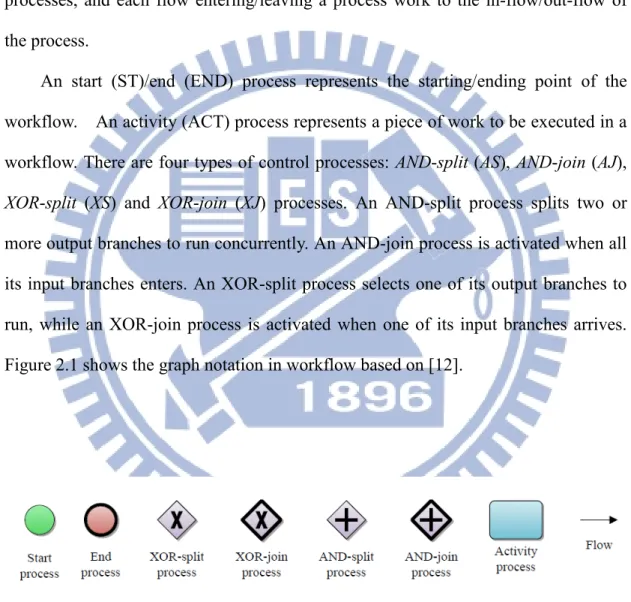
A workflow is composed of processes and flows [12], where processes are connected by flows. Each process is in charge of start, end, control and activity processes, and each flow entering/leaving a process work to the in-flow/out-flow of the process.
An start (ST)/end (END) process represents the starting/ending point of the workflow. An activity (ACT) process represents a piece of work to be executed in a workflow. There are four types of control processes: AND-split (AS), AND-join (AJ),
XOR-split (XS) and XOR-join (XJ) processes. An AND-split process splits two or
more output branches to run concurrently. An AND-join process is activated when all its input branches enters. An XOR-split process selects one of its output branches to run, while an XOR-join process is activated when one of its input branches arrives. Figure 2.1 shows the graph notation in workflow based on [12].
Figure 2.2 The blocks in a workflow
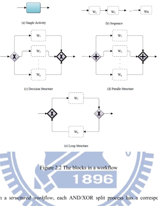
In a structured workflow, each AND/XOR split process has a corresponding AND / XOR join process to form a block [12]. All the processes between the start and end process in a structured workflow are organized with the blocks shown in Figure 2.2. In figure 2.2(a) indicates there is only an activity process. Figure 2.2(b) indicates a sequence of blocks W1, W2,..., Wn. Figure 2.2(c) indicates a decision to select one of
the blocks W1,W2, …, Wn to be executed. Figure 2.2(d) indicates a parallel structure
that all the blocks W1,W2, …, Wn are executed simultaneously. Figure 2.2(e) indicates
a loop structure where the entrance is an XOR joint process and output is an XOR split process, where the inner branch is the branch to execute the loop continually and
outer branch is the branch to execute after the loop stops.
Besides, a process is reachable from the other one if there is a path from the latter to it. Two processes are parallel if they reside in different branches of a parallel structure, and are exclusive to each other if they reside in different branches of a decision structure.
2.2 A temporal structured workflow
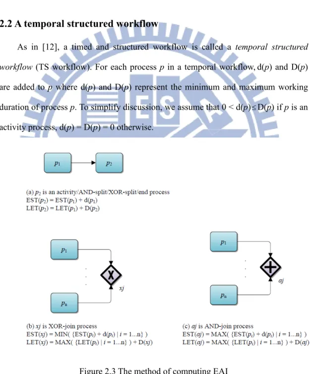
As in [12], a timed and structured workflow is called a temporal structured
workflow (TS workflow). For each process p in a temporal workflow,d(p) and D(p) are added to p where d(p) and D(p) represent the minimum and maximum working duration of process p. To simplify discussion, we assume that 0 < d(p)≤D(p) if p is an
activity process, d(p) = D(p) = 0 otherwise.
The Estimated Active Interval (EAI) of a process is a time interval indicating when the process can be initialized and when it has to be terminated. For each process
p in a TS workflow, EAI(p) = [EST(p), LET(p)] is a time interval where EST(p)
indicates the earliest time p can be initialized and LET(p) indicates the latest time p must be terminated. Figure 2.3 shows how to calculate EAI of a process.
On the other hand, the parallel processes in a TS workflow would not be possibly executed at the same time if their working durations do not overlap. Two processes p and q in a TS workflow are concurrent if p and q are parallel, and EAI(p) and EAI(q) are overlapped, p and q are sequential if p is reachable to q or q is reachable to p. Let processes p, q are both selected to execute during run-time, and q is reachable from p,
q cannot be executed before p. On the other hand, if p and q are parallel, and EAI(p)
is before EAI(q), p is also executed before q. For both circumstances above, p is before q, and there is no operation working on the same artifact at the estimated time interval before p’s EAI and after q’s EAI, p is said to be a immediate successor of q, q is a immediate predecessor of p.
2.3 Artifact operations and anomalies
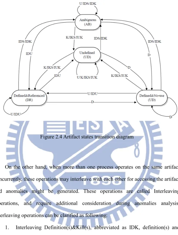
As in [12], an activity process in a TS workflow may operate an artifact with the following way(s): define (Def), use (Use) and kill (Kill). Def operation is to assign a value to the artifact, Use operation is to reference the artifact, and Kill operation is to delete value of the artifact. A process may also do nothing (Nop) on an artifact.
As in [12], an artifact in a TS workflow is initially stated undefined (UD), and turns to defined&no-use (DN) after it is defined. When a DN artifact is used, it turns to defined&reference (DR). Figure 2.4 shows the state changes of an artifact due to the artifact operations.
Figure 2.4 Artifact states transition diagram
On the other hand, when more than one process operates on the same artifact concurrently, these operations may interleave with each other for accessing the artifact and anomalies might be generated. These operations are called Interleaving Operations, and require additional consideration during anomalies analysis. Interleaving operations can be clarified as following:
1. Interleaving Definition(s)&Kill(s), abbreviated as IDK, definition(s) and kill(s).
2. Interleaving Definitions, abbreviated as IDS, multiple definitions, but no kill.
3. Interleaving Kill(s), abbreviated as IKS, multiple kills, but no definition. 4. Interleaving Definition&Usage(s), abbreviated as IDU, one definition, no
5. Interleaving Usage(s)&Kill, abbreviated as IUK, one kill, no definition, and at least one usage.
6. Interleaving Usages, abbreviated as IUS, multiple usages only.
Artifact anomalies can be generated due to structural and temporal relationships between processes. In [12], there are four types of anomalies: Useless Definition,
Undefined Usage, Null Kill and Ambiguous Usage. Useless Definition occurs when
killing or defining a DN artifact makes the previous definition useless because the definition is destroyed (or redefined) without any usage. Undefined Usage occurs when using an UD artifact is an error leading to faulty execution. It is necessary to be handled by the designers. Null Kill occurs when a null kill represents a process trying to remove an inexistent definition. For instance, kill a UD artifact. Ambiguous Usage occurs when an ambiguous usage means that an activity process uses an artifact which is ambiguous in definitions or in states. For instance, the direct usage of an AB artifact is an ambiguous usage.
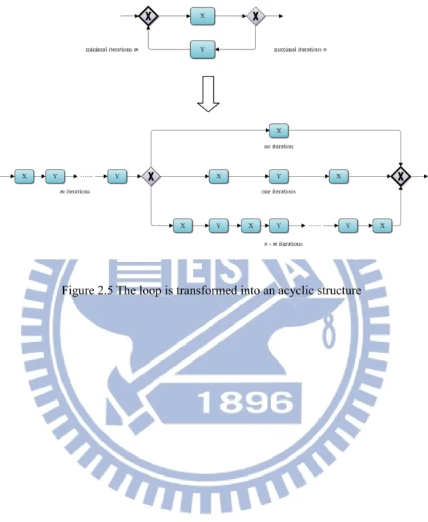
2.4 Loop reduction
For the loop structure, there are several approach [8][9][10]. These approaches all assume that there is at least zero time of execution. However, they do not consider the case which has at least k turns, k > 0. In Figure 2.5, X and Y represent the blocks in a TS workflow and the numbers of potential minimal and maximal iterations are m and n, where both numbers are larger than zero. The loop graph can be transformed as the lower graph, where the left sequence structure represents that a sequence of m blocks, and the right decision structure represents a loop structure at most (n - m) turns as in [12]. The transforming process is named as transformation of cyclic workflow to acyclic workflow (TCA).
Chapter 3 Temporal Computation for TS Workflow
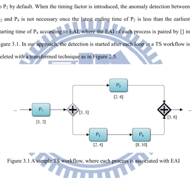
The anomaly detection techniques presented in previous approaches have some defects because the time interval consideration is not enough. For instance, there is no temporal issue consideration as in figure 3.1, processes P3 and P4 are both concurrent
to P2 by default. When the timing factor is introduced, the anomaly detection between
P2 and P4 is not necessary once the latest ending time of P2 is less than the earliest
starting time of P4 according to EAI, where the EAI of each process is paired by [] in
figure 3.1. In our approach, the detection is started after each loop in a TS workflow is deleted with a transformed technique as in Figure 2.5.
Figure 3.1 A sample TS workflow, where each process is associated with EAI
3.1 Level Computation for Processes
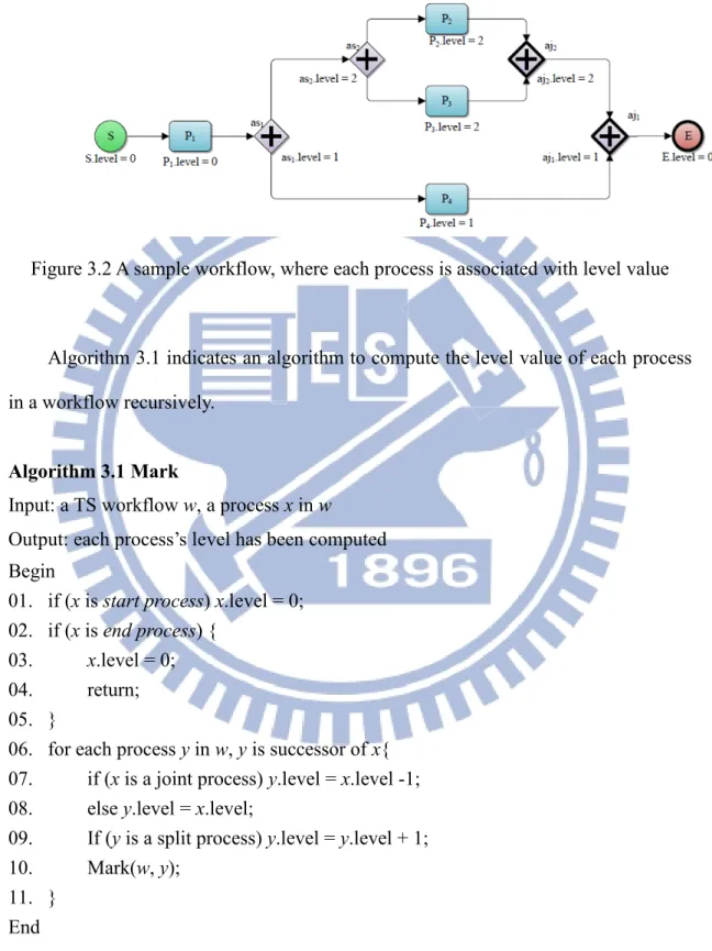
To identify the split process and corresponding joint process more clearly in a TS workflow, we associate each process with the attribute level in addition. For a parallel or exclusive structure, its split/joint process and the activity processes between them are associated with a common level value. When an exclusive/parallel structure is nested in another exclusive/parallel, the level of processes between the former is the
level of processes between the latter plus one. For example, P1’s level is 0 in figure
3.2, the level of as1, aj1 and P4 are 1, and the level of as2, aj2, P2, P3 are 2.
Figure 3.2 A sample workflow, where each process is associated with level value
Algorithm 3.1 indicates an algorithm to compute the level value of each process in a workflow recursively.
Algorithm 3.1 Mark
Input: a TS workflow w, a process x in w
Output: each process’s level has been computed Begin
01. if (x is start process) x.level = 0; 02. if (x is end process) {
03. x.level = 0;
04. return; 05. }
06. for each process y in w, y is successor of x{ 07. if (x is a joint process) y.level = x.level -1; 08. else y.level = x.level;
09. If (y is a split process) y.level = y.level + 1; 10. Mark(w, y);
11. } End
In each turn, the algorithm is instantiated with an input process x. In the first turn, the algorithm starts from the starting process. When x is an end process, there is no further recursion of Mark. For the rest processes, the recursion is done to each of its succeeding process(es). In lines 6-7, for each successor of x, named by y, the level of
y is assigned as (x.level – 1) if x is a joint process, x.level otherwise. In lines 10-11, y.level is defined as (y.level + 1) if x is split process.
For the workflow in Figure 3.2, obviously, s.level is assigned as 0 in line 1. P1.level is assigned as 0, and Mark(w, P1) is called in the first turn. In Mark(w, P1),
as1.level is assigned as 1, and Mark(w, as1) is called. In Mark(w, as1), i.e., 2nd turn,
as2.level is assigned as 2, and then Mark(w, as2) is called. After Mark(w, as2)
completes, P4.level is associated as 1 and Mark(w, P4) is called. In Mark(w, as2),
P2.level is assigned as 2, and Mark(w, P2) is called. After the level of aj2, aj1 and end
process are computed, the algorithm goes back to Mark(w, as2) to compute P3.level,
and Mark(w, aj2) is called again. Finally, the algorithm calls Mark(w, P4), and then
Mark(w, aj1) is called again.
Although algorithm 3.1 can compute the level of each process, however some recursive calls may be useless and redundant at line 10. For example, applying algorithm 3.1 on the workflow w in Figure 3.2, the calls, Mark(w, P2) and Mark(w, P3)
both compute aj2.level but derives the same value. To eliminate the defect in
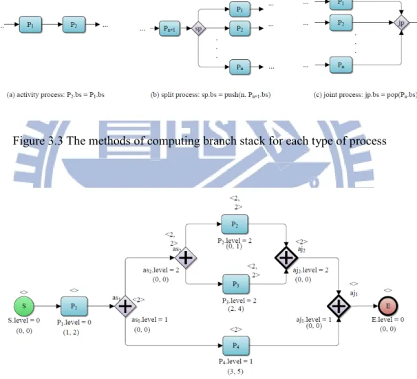
algorithm 3.1, we introduce the branch stack (bs) into each process. The branch stack (bs) of a process p is expressed with p.bs. The branch stack of a process p is defined as followings: (1) when p is an activity process, p’s bs is equal to the bs of its predecessor. (2) when p is a split process, p’s bs is equal to the bs of p’s predecessor pushed with the number of p’s split branches. (3) when p is a joint process, p’s bs is equal to the bs of p’s predecessor popped out one number. Figure 3.3 shows how to calculate the bs of each process. Figure 3.4 shows the branch stack with each process
from the workflow in Figure 3.2. For example, the branch stack associated with s and P1 are empty. The branch stack associated with as1 and as2 are <2> and <2, 2>
respectively. The branch stack associated with P2, P3 and P4 are <2>, <2> and <2, 2>
respectively. The branch stack associated with aj1 and aj2 are <> and <2> respectively.
Figure 3.3 The methods of computing branch stack for each type of process
Figure 3.4 The branch stacks attached on each process in workflow in Figure 3.2
Thus, we improve algorithm 3.1 by adding the branch stack to a process. Algorithm 3.2 shows how to compute the level of each process with branch stack.
Algorithm 3.2 ComputeLevel
Input: a TS workflow w, a process x in w
Output: each process’s level has been computed
01. Let each process’ bs and level be empty and zero respectively; 02. Let x be the start process in w;
03. Let q be an empty queue of processes; 04. enqueue(q) with x;
05. While( q is not empty ){ 06. y = dequeue(q);
07. if (y is not the end process){
08. For each successor z of y in w{
09. if (y is a joint process ) z.level = y.level -1; 10. else z.level = y.level;
11. Switch(z){
12. Case 1 “split process”:
13. z.bs = the stack copied from y.bs
14. push the number of split brnaches of z on z.bs; 15. z.level = z.level + 1;
16. enqueue(q) with z; 17. Case 2 “joint process”:
18. if( z.bs is empty ) z.bs = y.bs; 19. z.bs.top --;
20. if( z.bs.top == 0 ) { 21. pop(z.bs);
22. enqueue(q) with z; 23. }
24. Case 3 “other process”: 25. z.bs = y.bs; 26. enqueue(q) with z; 27. } 28. } 29. } 30. } End
Algorithm 3.2 stops when q is empty. In the while loop (lines 6-30), the successors of y is enqueued into queue q at line 16, 22, 26. The branch stack in Algorithm 3.2 is used to guarantee when starting to compute the data of a joint process, the data of its predecessors are derived. In lines 13-16, if z is a split process,
z.bs is a stack copied from y.bs and then pushed the number of split branches of z. In
lines 17-23, a joint process z in each turn is processed, z.bs.top is decremented by 1 at line 19. In the first turn, z.bs is initialized by y.bs at line 18. In the last turn z is processed, i.e., z.bs.top = 0, z.bs is popped and z is enquened into q in lines 20-23. The enqueue/dequeue operations on q make sure that (1) all the incoming branches of a joint process completes since its bs is zero then. (2) a process is enqueued once all its predecessors are passed. (3) the bs of a joint process in generated with the (number of its input branches – 1), since the first branch is passed. Thus, the guarantee succeeds.
For example, when applying algorithm 3.2 on the workflow in Figure 3.4, the algorithm enqueue start process into q at line 4. Considering the computation of while loop, in the first turn, P1.level is assigned as 1, q = <P1> after the first turn. In the fifth
turn, P4 is dequeued from q, then aj1.bs = <2>, and aj1.bs is assigned as <1>, q = <P2,
P3> after fifth turn. In the eighth turn, aj2 is dequeued from q, then aj1.bs = <0>, aj1 is
enqueued into q. In the next turn, aj1 is dequeued from q, then the end process' level is
computed. Finally, while loop stops because end process has no successor.
3.2 Removing Loop(s) in a Workflow
In section 2.4, we present a method to transform a simple cyclic workflow into an acyclic structure one by booting the method shown in Figure 2.5. Thus, the acyclic structure in the lower-level graph, as in Figure 2.5, can be applied to represent loop structure executing at least m times and at most n times.
To identify whether a pair of split/joint processes is a loop structure in a structured workflow, we introduce the attribute loop to both split and joint processes of a loop structure to indicate whether they represent a common loop. When the loop attribute of both XOR processes is true, the XOR structure represents a loop structure, not, otherwise. To travel each loop structure in a structured workflow, we introduce two loop stacks in Algorithm 3.3. When the transformation of a loop or its descendent loop is being handled, the loop stack of split process (lss) represents a stack of XOR split processes of a loop structure, the loop stack of joint process (lsj) represents a stack of XOR joint processes of a loop structure. Algorithm 3.3 applying the structure in Algorithm 3.2, shows how to transform a structured workflow into an acyclic workflow based on TCA in Figure 2.5.
Algorithm 3.3 Remove-Loop
Input: a TS workflow w
Output: an acyclic TS workflow w’ transformed from w Begin
01. Let each process’ bs be empty; 02. Let x be the start process in w;
03. Let q be a queue of processes and empty; 04. enqueue(q) with x;
05. Let lss and lsj be empty initially; 06. While( q is not empty ){
07. y = dequeue(q);
08. For each successor z of y in w{
09. if (y is an XOR split process with true loop and z is on the outer 10. branch)
11. else{
12. Switch(z){
13. Case 1 “ AND and XOR split process with loop is false”: 14. z.bs = the stack copied from y.bs, then pushed the
15. number of split branches of z; 16. enqueue(q) with z;
17. Case 2 “AND and XOR joint process with loop is false”: 18. if (z.bs is empty) z.bs = y.bs; 19. else z.bs.top --; 20. if( z.bs.top == 0 ) { 21. pop(z.bs); 22. enqueue(q) with z; 23. }
24. Case 3 “XOR split process with loop is true”: 25. push(lss) with z;
26. enqueue(q) with z;
27. Case 4 “XOR joint process with loop is true”: 28. if( lsj.top == z ){
29. Pop(lsj); 30. n = pop(lss);
31. Transform cyclic structure between n and z into an 32. acyclic structure by TCA;
33. Link m to n’s successor on outer branch; 34. revise m.bs; 35. enqueue(q) with m; 36. } 37. else{ 38. push(lsj) with z; 39. enqueue(q) with z; 40. }
41. Case 5 “other process”: 42. z.bs = y.bs; 43. enqueue(q) with z; 44. } 45. } 46. } 47. }
End
Algorithm 3.3 stops when q is empty at line 6. Cases 1, 2 and 5 in Algorithm 3.3 are similar to Algorithm 3.2. Case 3 and 4 in Algorithm 3.3 works for a pair of split/joint processes forming a loop structure. To prevent the successor on the outer branch of a loop from begging computed before loop is transformed, line 9 checks and detects such a case in switch. To simplify our explanation, let xs and xj represent input a pair of split/joint processes. In Case 4, xj is pushed into lsj and z is enqueued into q in lines 38-39 if lsj.top != xj. lsj.top == xj, indicates that xj is now handled at the second time and all the processes between xj and xs are traveled already, thus a loop structure between xs and xj is transformed by TCA in lines 31-32. Lines 33-35 enqueues the joint process of the transformed acyclic structure into q, and revise the bs of the joint process as to its successor. Case 3 pushes xs into lss and enqueues z into q in lines 25-26. Moreover, if there is a loop contained, son loop do TCA later than the other loop because of the operation of lss and lsj. The split/joint processes of a loop in lss/lsj are pushed earlier than those of the other loop. Thus, TCA is applied on the inner loop earlier (due to pop order).
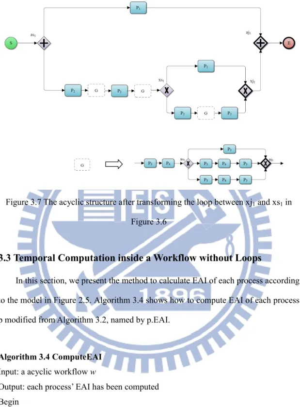
For instance, the loop starting at xs1 and ending at xj1contains the loop starting at xs2 and ending at xj2 in Figure 3.5. Algorithm 3.3 transforms the latter by TCA as shown in Figure 3.6. Next, Algorithm 3.3 transforms the former in Figure 3.6 by TCA as shown in Figure 3.7, where the block G in the lower graph shows the transformed acyclic structure.
Figure 3.5 A sample workflow owns a loop (between xj1 and xs1) containing another
loop(between xj2 and xs2)
Figure 3.6 The acyclic structure after transforming the loop between xj2 and xs2 in
Figure 3.7 The acyclic structure after transforming the loop between xj1 and xs1 in
Figure 3.6
3.3 Temporal Computation inside a Workflow without Loops
In this section, we present the method to calculate EAI of each process according to the model in Figure 2.5. Algorithm 3.4 shows how to compute EAI of each process p modified from Algorithm 3.2, named by p.EAI.
Algorithm 3.4 ComputeEAI
Input: a acyclic workflow w
Output: each process’ EAI has been computed Begin
01. Let each process’ bs and EAI be empty and [0, 0] respectively; 02. Let x be the start process in w;
03. Let q be a queue of processes and empty; 04. enqueue(q) with x;
05. While( q is not empty ){ 06. y = dequeue(q);
07. if (y is not end process){
08. For each successor z of y in w{ 09. Switch(z){
10. Case 1 “split process”:
11. z.bs = the stack copied from y.bs, then pushed the
12. number of split branches of z; 13. EST(z) = EST(y) + d(y);
14. LET(z) = LET(y) + D(z); 15. enqueue(q) with z; 16. Case 2 “joint process”:
17. if( z.bs is empty) z.bs = y.bs; 18. else z.bs.top --;
19. if( z.bs.top == 0 ) { 20. pop(z.bs);
21. If( z is an AND joint process ){
22. EST(z) = MAX{ EST(m) + d(m) | m is a 23. predecessor of z }; 24. LET(z) = MAX{LET(m) | m is a
25. predecessor of z } + D(z);
26. }
27. else{
28. EST(z) = MIN{ EST(m) + d(m) | m is a 29. predecessor of z }; 30. LET(z) = MAX{LET(m) | m is a 31. predecessor of z } + D(z); 32. } 33. enqueue(q) with z; 34. }
35. Case 3 “other process”: 36. z.bs = y.bs;
37. EST(z) = EST(y) + d(y); 38. LET(z) = LET(y) + D(z); 39. enqueue(q) with z;
40. } 41. } 42. } 43. } End
Algorithm 3.4 stops when q is empty; its main body is similar to Algorithm 3.2. In Algorithm 3.4, Case 1 and 3 compute the EAI of processes by TCA. Case 2 (joint process) is clarified into two sub cases, AND and XOR joint processes, to compute z’s EAI according to its predecessors in lines 21-32 when EAI of its all predecessors is computed once z.bs.top = 0 at line 19.
After a working duration of a process p, (D(p), d(p)), is added to p in the workflow in Figure 3.2, the workflow is shown in Figure 3.8. After a EAI of a process
p, (EST(p), LET(p)), is added to p in the workflow in Figure 3.8, the workflow is
shown in Figure 3.9.
When applying Algorithm 3.4 on the workflow in Figure 3.8, the algorithm pushes the start process into q at line 5. The computations for the rest are done in while loop (lines 5-43). After the first turn of the while loop, P1.EAI = [0, 2] and q =
<P1>. After the sixth turn of the while loop, aj2.bs.top = 1, q = <P3>. At the seventh
turn, aj2.bs.top = 0 is executed at line 18, then aj2.EAI is computed in lines 21-22:
EST(aj2) = MAX{EST(p2), EST(p3)} = MAX{1, 3} = 3, and LET(aj2) =
MAX{EST(p2), EST(p3)} + D(aj2)= MAX{3, 6} + 0 = 6, thus aj2.EAI = [3, 6]. After
the next turn, aj1.EAI = [4, 7] according to P4 and aj2. At the final trun, EAI of end
Figure 3.8 The workflow in Figure 3.2 which duration is attached to each process
Chapter 4 Anomaly Detection in a TS Workflow
In this chapter, we present several algorithms to detect anomalies based on our model of workflow. Section 4.1 presents a batched approach of anomaly detection. The modifications of a TS workflow can be classified into four categories to simplify the discussion: (1) Insertion/deletion of a pattern (2) Insertion/deletion of an artifact operation (3)Modification of (min, max) time for a process (4) Modification of (min, max) turns for a loop。Section 4.2 presents the incremental analysis correspondingly.
4.1 Anomaly Detection in a Batch
A static anomaly detection can be defined to find out the anomal(ies) in a TS workflow. Previous work [12] presents an algorithm of a batched detection of artifact anomaly in a workflow, but the algorithm is too rough to indicate the timing correctness. For example, the loop-reduction analysis is incomplete. In the algorithm, it does not count the minimum turns in a loop, while the specification of such a number is done on a TS workflow. Algorithm 4.1 is applied to improve these deficiencies.
In algorithm 4.1, we define and analyze a corresponding workflow (discussed in Section 3.3) to the one constructed by designer. Such an analysis is called a batched analysis. Since an XOR or AND structure might contain a branch of no operation, let such a branch be called an XBB/ABB in an XOR/AND structure. To simplify the discussion, an XBB is also introduced for the loop in the corresponding workflow.
Algorithm 4.1 BatchedAnomalyDetection
Input: a TS workflow w Output: anomalies
Begin
01. Removing-Loop(w); //algorithm 3.3 02. ComputeEAI(w); //algorithm 3.1 03. ComputeLevel(w); //algorithm 3.2 04. Let x be the start process in w;
05. Let q be a queue of processes and empty; 06. enqueue(q) with x;
07. While (q is not empty){ 08. y = dequeue(q);
09. For each successor z of y in w{ 10. Switch(z){
11. Case 1: “split process”:{
12. z.bs = y.bs, and pushing the number of split branches of z
13. into y.bs; 14. enqueue(q) with z}; 15. Case 2: “joint process”:{
16. if( z.bs is empty) z.bs = y.bs; 17. else z.bs.top --;
18. if( z.bs.top == 0 ) { 19. pop(z.bs);
20. enqueue(q) with z; 21. }};
22. Case 3: “other process”:{ 23. z.bs = y.bs;
24. A = {a| a is an artifact in w, z has operation on a};
25. S = {(p,a, o) | p is a process in w, p is before z , a is operated 26. with o in p, where a A, o {Def, Kill, Use} } 27. where (p, a, o)’s are derived using traveling the 28. Mechanism as in Algorithm 3.2;
29. Do{
30. S’ = {pa | pa S, pa.p is a immediate predecessor of z}; 31. G = the set of elements derived in Section 4 in [7] 32. For each (g, a), where g G and α A ) {
33. Switch(g, a){
34. Case 1:”the operations in g are IDS/IDK “: 35. Useless Definition occurs;
36. if (the operation on a in z is Use) 37. Ambiguous Usage occurs;
38. Case 2:” the operations in g are IKU/IKS “: 39. Null Kill occurs;
40. if (the operation on a in z is Use) 41. Undefined Usage occurs;
42. else if (the operation on a in z is Kill) 43. Null Kill occurs;
44. Case 3:” the operations in g are IDU “: 45. if (the operation on a in z is Def ) 46. Useless Definition occurs; 47. Case 4:” the operations in g are Def “: 48. if (the operation on a in z is Def ) 49. Useless Definition occurs; 50. if (the operation on a in z is Kill) 51. Useless Definition occurs; 52. Case 5:” the operations in g are Kill “:
53. if (the operation on a in z is Kill) Null Kill occurs; 54. }};
55. S’’ = S;
56. S = S \ {pa| pa S’, pa.p is contained in an XOR 57. structure X, X has an XBB,
58. and X’s level == pa.p.level }; 59. }while (S S’’); 60. enqueue(q) with z} 61. } 62. } 63. } End
In Algorithm 4.1, the loops in the workflow w are replaced with acyclic structure by using Algorithm 3.3 at line 1. Algorithms 3.1 and 3.2 are applied to compute the level and EAI of each process in lines 2-3. Algorithm 4.1 adopts a similar traveling method as in Algorithm 3.3, so that we do not explain in details for the structure of both “while” and “for” loops in lines 4-63. However, the computation at each turn of the “for” loop is based on the type of process z. The cases for split and joint processes are handled in lines 11-21 and not discussed in details since it is similar to the Algorithm 3.3 containing the anomaly detection steps working on the process z being handled.
For each process, neither split nor joint, the computations are done in lines 22-61. At line 24, set A is calculated to contain the artifacts operated in the process z. For each artifact, such as a, in A, we define a three tuple (p, a, o) named as pao to simplify our discussion, where p is a process before z, and o is the activity (operation) working on a at p, i.e., o is one of activities, Def, Kill and Use. The pao of each artifact in A is calculated and all the pao’s derived are form as a set S in lines 25-28, where the details of how to get the processes are skipped because we adopt a traveling method in Algorithm 3.2 which has been shown correct.
The do-while loop detects the potential anomaly(ies) due to blank branches in lines 29-59. At line 30, All pao’s in S whose p is a immediate predecessor of z are collected as a set S’. At the end (lines 55-59) of each turn of the loop, if S is changed, S’ contains at least one XOR element that has a blank branch and the next turn starts. Otherwise, the loop terminates.
In each turn, line 31 is responsible for identifying concurrency for the processes of pao in S’. G is a set of elements which are the set containing pao’s. After G is constructed at line 31, G has the following properties:
1. For each element g in G, if pa1 and pa2 belong to g, pa1.p and pa2.p are
concurrent.
2. For any two elements g1 and g2 in G, g1 g2 and g1 g2
3. For any two elements pa1 and pa2 in S’,
a. If pa1.p and pa2.p are concurrent, G has an element containing both
pao1 and pao2.
b. If pa1.p and pa2.p belong to two distinct elements in G and pa1.p pa2.p,
pa1.p and pa2.p are not concurrent.
However, the calculation of G is a NP problem: maximum clique problem, and the lemma 2 in Section 4 in [7] is adopted at line 31.
Lines 32-53 analyze each pair (g, a) where g G and a A. According to the discussion in Chapter 2, all possible pairs for (g, a) can be classified into five cases, including single operation and the corresponding operations are described correspondingly as below:
1. The component elements in g are IDS/IDK for a, g itself contains Useless Definition anomaly. Besides, if artifact a has Use operation in g, there is an anomaly of ambiguous use. The handling operations are done in lines 35-37.
2. The operations in g are IKU/IKS. g itself contains an anomaly of Null Kill. If there is a Use operation on a in z, it causes anomaly of Undefined Usage. Otherwise, if there is a Kill operation on a in z, it causes anomaly of Null Kill. The handling operations are done in lines 39-43.
3. The operations in g are IDU. If artifact a has Def operation in z, there is anomaly of Useless Definition. The handling operations are done in lines 44-45.
4. The operations in g is Def. If artifact a has Def operation in z, it causes anomaly of Useless Definition. Otherwise, if artifact a has Kill operation in
z, it causes anomaly of Null Kill. The handling operations are done in lines
47-51.
5. The operation in g is Kill. If artifact a has Kill operation in z, it causes anomaly of Null Kill. The handling operation is done line 53.
Finally, the content of S is copied to S’’ at line 55. For each process of pao in S’, if there exists an XOR structure X containing the process of pao, X is associated with the same level of the process, and X has XBB, the pao’s in S’ whose process is contained in X are removed from S in lines 56-58. Now, at line 59, that S equals to S’’ indicates there is no blank branch found in XOR structures in lines 55-58. Thus, the do-while loop terminates when the content of S and S’’ are equal, continues otherwise. After the loop, enqueuing z into q at line 60 is the last step of the handling a successor
z of process y.
In algorithm 4.1, lines 23-60 are responsible to find out all the artifact anomalies associated with the operation in the concerned process. The loop defined at line 7 shall pass all processes. In other word, all the processes except split/joint process are examined. Thus, all the anomalies in workflow are detected by algorithm 4.1.
For instance, a sample of TS workflow associated with operation working on an artifact a in Figure 4.1, Algorithm 4.1 would detects Useless Definition at P3 because
Figure 4.1 A sample TS workflow associated with operation working on an artifact a
4.2 Incremental anomaly detection
Each loop in a workflow is transformed into an acyclic structure based on the definition of Section 2.4. Thus, each TS workflow diagram being edited has a corresponding acyclic workflow diagram, named as CTS workflow. Section 4.2 presents a set of algorithms for incremental anomaly analysis of the CTS, which is done once the operation edition on artifacts inside a single process or a structure modification such as insertion/deletion completes in the original workflow.
4.2.1 Detection inside a TS workflow
Our incremental analysis works based on divide and conquer mechanism; it contains three steps, step by step:
1. analyzing the block containing edited process. 2. analyzing the rest of workflow.
3. Computing the anomalies according to the results of 1 and 2.
associated with each process p in a workflow w, besides level, working duration, and EAI which are described in Chapters 2 and 3. The definitions of these attributes are defined below:
1. There are five process types: asp, ajp, xsp, xjp and ap; asp/ajp and xsp/xjp indicate split/joint process of AND and XOR respectively, and ap indicates activity process.
2. AOSetp = {(a, o) | a is an artifact in w, operation o works on a in p, and o
{Def, Kill, Use}}.
3. ImmeSucprepresents the set of process(es) of which each has an operation on a, and there is an empty path on a from p to the process. Moreover we define ImmeSucp(Def) = {q | q ImmeSucp , the operation of a in q is Def}, ImmeSucp(Kill) = {q | q ImmeSucp , the operation of a in q is Kill}, ImmeSucp(Use) = {q | q ImmeSucp , the operation of a in q is Use}.
4. ImmePrep represents the set of process(es) of which each has an operation on a, and there is an empty path on a from the process to p. we define the following sets: ImmePrep (Def) = {q | q ImmeSucp, the operation of a in
q is Def}, ImmePrep(Kill) = {q | q ImmeSucp , the operation of a in q is Kill}, and ImmePrep(Use) = {q |q ImmeSucp , the operation of a in q is Use}.
An incremental analysis in general is to analyze abnormal operation behavior due to an operation in a workflow editor [12]. Because such an analysis has been shown to be an NP problem when a workflow contains a loop(s), we define a new incremental approach to simplify the work. In our work, when a TS workflow is modified (addition/deletion/modification a process) by user, our approach has a
corresponding modification in its CTS workflow to reduce the analysis work and thus waiting time for designer.
To simplify the discussion, the incremental analysis algorithms presented are based on each of the following four types of edit activities:
1. Insertion/deletion of a workflow template indicates to insert/delete a Loop/AND/XOR structure or an activity process.
2. Insertion/deletion of an operation on some artifact. 3. modification of (min, max) turns of a loop.
4. modification of (mix, max) time interval of a process.
Because each loop in a TS workflow has a corresponding complicated acyclic structure in its CTS workflow, when an insertion/deletion/modification of a loop in a TS workflow occurs, the target CTS workflow has to be modified first in order to follow the reduction principle in Section 2.4 correspondingly. Insertion/deletion of an operation on an artifact a is to add/delete an operation on a in an activity process p. To simplify the analysis, it is assumed that an artifact has at most one operation in an activity process. After an operation on a is inserted/delete in p, there is one operation/no operation for a in p and corresponding process(es) in the CTS workflow.
The modification of (min, max) turns for a loop is to increase/decrease the minimum/maximum turns of a loop. As mentioned before, a loop can be transformed into an acyclic structure when a designer adds the loop into a TS workflow (Section 2.4). It has to modify the corresponding CTS workflow for a modification of (min, max) turns of a loop. The modifications of a loop is done by increasing/deleting for one of both of (min, max), and one increases and the other decreases. The modification of a CTS workflow can be discussed according to the followings:
due to:
a. max is of no change or incremented, but min is incremented lower, of no change, or decremented.
b. max is decremented, but min is decremented larger. 2. The resulting value become smaller. This occurs due to:
a. max is of no change or incremented, but min is incremented larger. b. max is decremented, but min is incremented, of no change, or
decremented lower.
Modification of (min, max) time for a process is to change minimum/maximum working duration of an activity process. If a designer modifies the working duration of an activity process in a loop, it has to adjust the timing of the corresponding acyclic which contain this data in the CTS workflow.
It might update ImmeSucap and ImmePreap of a process p when an edit activity to artifact a occur somewhere else. In our approach, the analysis is focused on a workflow block, containing the process p being edited, and starts by computing ImmeSucap and ImmePreap according to the level of the block. Algorithm 4.2 computes ImmeSucap and Algorithm 4.3 computes ImmePreap. Because we analyze a workflow at a predefined level, obviously, some information need be modified due to an edit activity. The information modification related to the blank branches between p and p’ is done with Algorithm 4.4. which outputs a set of artifacts containing at least one operation in each branch between two input processes p and p’.
Both Algorithm 4.2 and Algorithm 4.3 work with input (w, a, p, p’), where w is a workflow, a is an artifact, and p and p’ are processes. Algorithm 4.2 starts the computation from p, decides whether to make a recursive based on p’, and terminates with output ImmeSucap. Input p’ in Algorithm 4.3 is a split process and the output is
ImmePreap.
Algorithm 4.2 ComputeImmediateSuccessor
Input: an acyclic TS workflow w, an artifact a, a process p, a joint process p’ Output: ImmeSucap
01. S = ;
02. if (p is a split process){
03. p’’ = the joint process corresponding to p;
04. if( p is an AND process){ 05. IfContinue = true;
06. For each successor of p, x{
07. T = Algorithm 4.2(w, a, x, p’’); 08. S = S T;
09. }
10. IfContinue = IfContinue && (T ); 11. }
12. else if (p is an XOR process){ 13. IfContinue = false;
14. For each successor of p, x{
15. T = Algorithm 4.2(w, a, x, p’’); 16. IfContinue = IfContinue || ( T ) ; 17. S = S T;
18. } 19. }
20. if (p’’ p’ && IfContinue is true) S = S Algorithm 4.2(w, a, the 21. successor of p’’, p’); 22. }
23. else if (p is an activity process){
24. if (p has operations on a) S = S { p}; 25. else{
26. p’’ = the successor of p;
27. S = S Algorithm 4.2(w, a, p’’, p’); 28. }
29. }
30. return S; End
Algorithm 4.2 terminates and returns an empty set at line 30 when p is a joint process. In the algorithm, the handlings of a process are divided into 3 categories: split, joint and activity. The decisions are made at lines 2 and 23. In the very beginning, a set S initialized as empty at line 1 and its value is used to be returned at line 30. If p is a split process, the related computations are done in Lines 3-21 where Line 3 assigns the corresponding joint of p to p’’, Lines 5-9 works for AND split, Lines 13-17works for XOR split, and Lines 20-21 make a recursive call to get the artifacts from current joint p” to p’ if p’’ is not p’.
For an AND split process, Line 5 makes a recursive call for each P’s successor. IfContinue is made true in case no branch contains operation on a as in Line 8. Lines 13-17 are in charge of the work for XOR split, where the recursion works for each of
p’s branches, IfContinue is true if there is a branch containing no work on a, and S is
the union of these returned value. Lines 24-27 works if p is an activity process. Finally, line 30 returns result. For instance, Algorithm 4.2 (w, a, as2, aj2) being called
in Figure 4.1 would output {P2, P3}.
In Algorithm 4.2, each process is touched at most once, thus the time complexity is O(n), n is the number of the processes in the workflow.
Algorithm 4.3 accepts (w, a, p, p’) input in the very beginning, where w is a workflow, a is an artifact, p is an input process for starting the execution and p’ is the split process used to decide the termination of the algorithm, and outputs ImmePreap. The algorithm works inside a workflow block of some level, or whose split process is
workflow w, input artifact a, p and p’.
Algorithm 4.3 ComputeImmediatePredecessor
Input: an acyclic TS workflow w, an artifact a, a process p, a split process p’ Output: ImmePreap
01. S = ;
02. if (p is a joint process){
03. if (p is an AND joint process){ 04. IfContinue = true;
05. For each predecessor of p, x{ 06. T = Algorithm 4.3(w, a, x, p’); 07. S = S T;
08. }
09. IfContinue = IfContinue && (T ); 10. }
11. else if (p is an XOR joint process){ 12. IfContinue = false;
13. For each predecessor of p, x{ 14. T = Algorithm 4.3(w, a, x, p’); 15. IfContinue = IfContinue || (T ); 16. S = S T;
17. } 18. }
19. p’’ = the split process corresponding to p;
20. if (p’’ p’ && IfContinue is true) S = S Algorithm 4.3(w, a, 21. predecessor of p’’, p’); 22. }
23. else if (p is an activity process){
24. if (a is operated in p) S = S { p}; 25. else{
26. p’’ = the predecessor of p;
27. S = S Algorithm 4.3(w, a, p’’, p’); 28. }
29. }
30. return S; End
Algorithm 4.3 has a similar but reverse control structure, compared with Algorithm 4.2. Both algorithms analyze the flow structure, however, Algorithm 4.3 replaces predecessor/successor with successor/predecessor in Algorithm 4.2. In other words, Algorithm 4.3 uses backward analysis, and does not analyze split process but returns empty set directly. Furthermore, the complexity of Algorithm 4.3 is O(n) too. For example, Algorithm 4.3 (w, a, as2, aj2) being called in Figure 4.1 would output
{P2, P3}.
4.2.2 Computing concurrent and nonempty set
Our incremental analysis works on a block of some level value. During the analysis, constructing/deleting a blank branch of the block might modify the anomalies due to predecessor/successor of current block. Algorithm 4.4 inputs a workflow w, and two processes p and p’, and returns a set of artifacts, which have no operations between p and p’. p’ in Algorithm 4.4 plays the same role in Algorithm 4.2.
Algorithm 4.4 ComputeNonEmpty
Input: an acyclic TS workflow w, a process p, a joint process p’ Output: The set of artifacts in w with no blank branches
Begin
01. if (p is a split process){ 02. S = ;
03. if (p is an AND process){
04. For each the successor of p, x,
06. }
07. else if (p is an XOR process){ 08. S = {a | a is an artifact in w}; 09. For each the successor of p, x,
10. S = S Algorithm 4.4(w, x, p’); 11. }
12. p’’ = the joint process corresponding to p;
13. if( p’’ p’) S = S Algorithm 4.4(w, the successor of p’’, p’); 14. }
15. else if( p is an activity process){ 16. p’’ = the successor of p;
17. S = {a | p has operation on a} Algorithm 4.4(w, p’’, p’); 18. }
19. else S = ; 20. return S; End
In the beginning, Algorithm 4.4 is given a workflow between (p, p’) where p/p’ is the split/joint process. If p is a split process, the algorithm decides whether to make a recursion according to the value of p’’. The algorithm terminates and returns the retsults calculated at line 20. Lines 2-18 adopts an if structure and dispatch the works when p is a split process. Lines 4-5 indicate the work for an AND process, the work unites the value of each subbranch of p by applying the Algorithm 4.4 and assigns the united results to S. Lines 8-10 do the work for an XOR process. Lines 9-10 intersect the value of each subbranch of p by applying the Algorithm 4.4 and assigns the united results to S. Let p’’ be a joint process corresponding to p at line 12. If p’’ is not p’, the self recursion is applied on the successor of p’’ at line 13. At line 15, if p is an activity process, line 16-17 unites S and artifacts with operations on p, and the self recursion is applied on p. Line 17 is correct even if p’’ is a joint process. Line 19 assigns empty
set to S if p is a joint process. Finally, line 20 returns the result.
In Algorithm 4.4, input n processes and each process is touched once, thus the time complexity is O(n) for input n processes.
For example, Figure 4.2 shows a workflow which has three artifact a1, a2 and
a3( blank indicating no operation). Algorithm 4.4(w, as1, aj1) being called in Figure
4.2 would output { a1, a3}.
Figure 4.2 A sample workflow which has three artifacts a1, a2 and a3( blank indicating
no operation)
Algorithm 4.5 is to find all processes in a branch. Algorithm 4.5 inputs a workflow w, two processes p and p’; it returns the set of activity processes between p and p’.
Algorithm 4.5 ComputeProcessBranch
Input: an acyclic TS workflow w, a process p, a joint process p’ Output: the set of activity processes between p and p’
Begin
02. else{
03. if (p is a split process){ 04. S = ;
05. For each the successor of p, x, S = S Algorithm 4.5(w, x, p’); 06. p’’ = the successor of the joint process corresponding to p;
07. }
08. else if( p is an activity process) { 09. S = {p}; 10. p’’ = the successor of p; 11. } 12. if( p’’ p’) S = S Algorithm 4.5(w, p’’, p’); 13. } 14. return S; End
Algorithm 4.5 adopts the same structure as in Algorithm 4.4. If p is a joint process, S is assigned as empty set at line 1. If p is a split process, the results of each successor of p are putted into S at line 5. If p is an activity process, S is assigned as {p} at line 9. Algorithm 4.5 recurs itself when the successor p’’ is not p’ at line 12, p’’ is assigned at line 6 and line 10. Line 14 returns the results.
In Algorithm 4.5, input n processes and each process is touched once, thus the time complexity is O(n) for input n processes.
Algorithm 4.6 inputs a workflow w and a process p, it returns the set of processes which are concurrent to p.
Algorithm 4.6 ComputeConcurrentProcess
Input: an acyclic TS workflow w, a process p
Output: The set of processes which are concurrent to p in w Begin
01. S = ;
03. while(p’.level > 0){
04. if(p’ is an AND split process) {
05. foreach successor of p’, x, if (x is not reachable to p){
06. S = S Algorithm 4.5(w, x, the joint process corresponding to p’); 07. }
08. }
09. p’ = the predecessor of p’;
10. }
11. S ={x| x S, EST(x) < LET(p) or EST(p) < LET(x)} 12. return S;
End
Algorithm 4.6 starts from current process and recurs itself till the level of p’s predecessor equals to zero. In Algorithm 4.6, s is initialized as an empty set (line 1). If
p is an AND split process, Algorithm 4.5 is called for the each successor of p, but the
predecessor of p, where another parameter is p’s corresponding joint process. The works are done as a while loop which stops when p’.level equals to zero. After getting all the process which might be parallel with p, line 11 filtering out those which cannot concurrent with p according to temporal information.
S is initially empty set at line 1. p’ is assigned as predecessor of p. Line 3 -10 is a while loop, if p’.level is greater than zero, it executes line 4-9. At line 4, if p’ is an AND split process, it inputs successors of p’ to Algorithm 4.5 at line 6 to get the processes in each branch, and the results is putted into S, but the branch containing p is not executed because we only need the processes which are parallel with p at line 5. At line 9, p’ is assigned as its predecessor. If p’.level equals to zero, it indicates no control block need to be inspected. Line 11 collects the processes which their EAI are overlaid with the EAI of p. Line 12 returns the set of processes which are concurrent to p. For instance, Algorithm 4.6(w, P4) being called in Figure 4.1 would output {P2,
P3}.
Algorithm 4.5 and Algorithm 4.6 can be improved. For instance, since the checking at line 11, Algorithm 4.6 is done for each process in the parallel branch of p. The checking can be done at each parallel process found to check whether its following process is parallel with p temporally. If the answer is not, it’s not necessary to continue the work for its successor. Thus, it saves the execution time.
Our incremental analysis of a TS workflow is classified into two steps:
1. For the edited process, we observe its immediate predecessor and immediate successor,
a. The loops in this workflow are removed and replaced by XOR structures in our discussion in Section 2.4.
b. It compares ImmeSuc and ImmePre of edited process to check what anomalies occur.
2. For the edited process, we find out the processes which are concurrent to the process by Algorithm 4.6. For each artifact a,
a. the operation in the edited process on a is Def, if there exists Def/Kill in these processes, Useless Definition occurs.
b. the operation in the edited process on a is Kill, if there exists Def/Kill/Use in these processes, Useless Definition/Null Kill/Undefined Usage occur.
c. the operation in the edited process on a is Use, if there exists Kill in these processes to cause Undefined Usage.
4.2.3 Anomaly detection with the algorithms in above two subsections
Consider the edit activities in a well-formed workflow editing environment, there are at least 5 types of editing activities, besides moving the cursor,