國
國
國 立
立
立 交
交
交 通
通
通 大
大
大
學
學
學
電
電
電信
信
信工
工
工程
程
程研
研
研究
究
究所
所
所
博
博
博 士
士
士
論
論
論 文
文
文
二
二
二元
元
元無
無
無
記
記
記憶
憶
憶通
通
通道
道
道的
的
的最
最
最佳
佳
佳極
極
極小
小
小區
區
區塊
塊
塊碼
碼
碼設
設
設計
計
計
Optimal Ultra-Small Block-Codes
for Binary Input
Discrete Memoryless Channels
研究生:林玄寅
指
導教授:
Stefan M. Moser
博士
陳 伯寧 博士
Optimal Ultra-Small Block-Codes
for Binary Input Discrete Memoryless Channels
國
國
國立
立
立交
交
交通
通
通大
大
大學
學
學
電
電
電信
信
信工
工
工程
程
程研
研
研究
究
究所
所
所
博
博
博士
士
士論
論
論文
文
文
A Dissertation
Submitted to Institute of Communication Engineering
College of Electrical and Computer Engineering
National Chiao Tung University
in Partial Fulfillment of the Requirements
for the Degree of Doctor of Philosophy
in
Communication Engineering
Hsinchu, Taiwan
研究生:林玄寅
指
導教授:莫詩台方 博士
陳 伯寧 博士
Student: Hsuan-Yin Lin
Advisors: Dr. Stefan M. Moser
Dr. Po-Ning Chen
Laboratory
Insititute of Communication Engineering National Chiao Tung University
Doctor Project
Optimal Ultra-Small Block-Codes
for Binary Input
Discrete Memoryless Channels
Hsuan-Yin Lin
Advisors: Prof. Dr. Stefan M. Moser National Chiao Tung University, Taiwan Prof. Dr. Po-Ning Chen National Chiao Tung University, Taiwan Graduation Prof. Dr. Ying Li Yuan Ze University, Taiwan
Committee: Prof. Dr. Mao-Chao Lin National Taiwan University, Taiwan Prof. Dr. Chung-Chin Lu National Tsing Hua University, Taiwan Prof. Dr. Hsiao-Feng (Francis) Lu National Chiao Tung University, Taiwan Prof. Dr. Yu Ted Su National Chiao Tung University, Taiwan Prof. Guu-Chang Yang National Chung Hsing University, Taiwan
Abstract
for Binary Input Discrete Memoryless Channels
Student: Hsuan-Yin Lin
Advisors: Dr. Stefan M. Moser
Dr. Po-Ning Chen
Institute of Communications Engineering
National Chiao Tung University
Optimal block-codes with a very small number of codewords are investigated for the binary input discrete memoryless channels. Those channels are the binary asymmetric channel (BAC), including the two special cases of the binary symmetric channel (BSC) and the Z-channel (ZC). The binary erasure channel (BEC) is a common used channel with ternary output. For the asymmetric channels, a general BAC, it is shown that so-called flip codes are optimal codes with two codewords. The optimal (in the sense of minimum average error probability, using maximum likelihood decoding) code structure is derived for the ZC in the cases of two, three, and four codewords and an arbitrary finite blocklength. For the symmetric channels, the BSC and the BEC, the optimal code structure is derived with at most three codewords and an arbitrary finite blocklength, a statement for linear optimal codes with four codes is also given.
The derivation of these optimal codes relies heavily on a new approach of constructing and analyzing the codebook matrix not row-wise (codewords), but column-wise. This new tool allows an elegant definition of interesting code families that is recursive in the blocklength n and admits their exact analysis of error performance that is not based on the union bound or other approximations.
研究生:林玄寅
指
導教授:莫詩台方 博士
陳伯寧 博士
國立交通大學電信工程研究所
摘要
在 這 篇 論 文 中 ,我們探討數種二元無記憶通道模式下的極小區塊碼 (ultra-small block code) 的最佳設計 (optimal design),所探討的二元無記憶通道模式包含:二元 非對稱通道 (binary asymmetric channel or BAC) 與二元輸入三元輸出的二元抹除通 道 (binary erasure channel or BEC)。針對前者,我們另將特別著重兩個特例,即二元 對稱通道 (binary symmetric channel or BSC) 與Z-通道 (Z-channel or ZC)。本研究中所 謂的最佳碼,指的是在最大概度解碼 (maximum-likelihood decoding) 法則下,可達最 低平均錯誤率的區塊碼設計。而所謂的極小區塊碼指的是碼字個數極小的情況,例 如 2、3 或 4 。
針對二元非對稱通道 (BAC),我們證明了當碼字個數為 2 時,相對碼 (flip codes) 為 最佳區塊碼設計。另外,針對二元非對稱通道 (BAC) 的特例Z-通道,我們在碼字個數 為 2、3、4 時,也提出給定任意碼長 (block length) 的最佳設計。而對於對稱式的通道, 例如二元對稱通道 (BSC) 與二元抹除通道 (BEC),我們針對碼字個數為 2 與 3 的情況 下,找到給定任意碼長的最佳碼的設計規律。此外針對這兩個對稱式的通道,在碼字個 數增加為 4 時,我們也設計了最佳的線性區塊碼 (linear block code)。
我們證明所設計的區塊碼可達最低的最大概度解碼錯誤率的主要關鍵技巧,乃是我們 使用新的區塊碼建構觀點。簡言之,我們不用傳統碼字 (codeword) 為基準的分析法則, 而是針對區塊碼矩陣採用以直列組合方式進行分析。這種新的分析方式可以精巧的定義 出必要的區塊碼類別, 使我們可用區塊碼的碼長遞迴的方式來建構碼,同時也讓我們可以 推導出區塊碼的平均錯誤率的精確公式,而不需依賴傳統的聯集上限 (union bound) 或是 其他所謂的錯誤率近似值的分析技巧。
First and foremost, I would like to express my deep and sincerest gratitude to Prof. Stefan M. Moser and Prof. Po-Ning Chen, my research advisers, for their insightful comments, patient guidance, enthusiastic encouragement and suggestions on any matter related this thesis. Without their help and support, this thesis would not be completed. Prof. Moser, who has supported me throughout my thesis with his patience and knowledge while al-lowing me the space to work in my own way. He always give me right instruction and impressed intuition guidance for the research path. He helped me get on the road to LA-TEX and provided an experienced ear for my doubts about writing a thesis. Prof. Chen’s strong insights in information theory and mathematics leads me in a right way for proofs in my research, and his plenty of experiences for proving mathematical theorems indicate me how to do theoretical research by perseverance. I have learned numerous principal things from them, not only doing research, but also the attitude in life.
I also want to thank all the members and alumni in our Information Theory LAB. They have helped me a lot in my oral presentation and oral defense. We do have a great time during my Ph.D. time.
I am very grateful to my girlfriend Yi-Wen Wu, she always encourage and accompany me when the depress time, without her support, this thesis can not be completed and I would not continue my dream to finish my Ph.D. thesis.
Finally I would also like to extend my thanks to my parents, they never push me to do what I don’t want to do. I am greatly indebted to my family.
Hsinchu, Taiwan 28 June 2013
Table of Contents X
1 Introduction 2
1.1 Introduction. . . 2
2 Definitions 6 2.1 Discrete Memoryless Channel . . . 6
2.2 Coding for DMC . . . 7
3 Channel Models 11 4 Preliminaries 15 4.1 Error Probability of the BAC . . . 15
4.1.1 Capacity of the BAC. . . 15
4.2 Error (and Success) Probability of the ZC . . . 16
4.3 Error (and Success) Probability of the BSC . . . 17
4.3.1 Capacity of the BSC . . . 17
4.4 Error (and Success) Probability of the BEC . . . 17
4.4.1 Capacity of the BEC . . . 18
4.5 Pairwise Hamming Distance . . . 18
5 A Counterexample 19 6 Flip Codes, Weak Flip Codes and Hadamard Codes 20 6.1 Characteristics of Weak Flip Codes . . . 25
7 Previous Work 29 7.1 SGB Bounds on the Average Error Probability . . . 29
7.2 Gallager Bound . . . 31
7.3 PPV Bounds for the BSC . . . 32
8 Analysis of the BAC 34
8.1 Optimal Codes . . . 34
8.2 The Optimal Decision Rule for Flip Codes . . . 35
8.3 Best Codes for a Fixed Decision Rule. . . 37
9 Analysis of the ZC 42 9.1 Optimal Codes with Two Codewords (M = 2) . . . 42
9.2 Optimal Codes with Three or Four Codewords (M = 3, 4) . . . 42
9.3 Error Exponents . . . 46
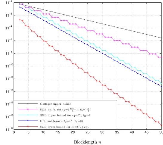
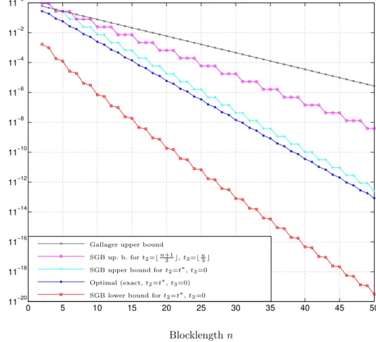
9.4 Application to Known Bounds on the Error Probability for a Finite Block-length . . . 46
9.5 Conjectured Optimal Codes with Five Codewords (M = 5) . . . 49
10 Analysis of the BSC 51 10.1 Optimal Codes with Two Codewords (M = 2). . . 51
10.2 Optimal Codes with Three or Four Codewords (M = 3, 4) . . . 51
10.3 Pairwise Hamming Distance Structure . . . 53
10.4 Application to Known Bounds on the Error Probability for a Finite Block-length . . . 55
11 Analysis of the BEC 59 11.1 Optimal Codes with Two Codewords (M = 2). . . 59
11.2 Optimal Codes with Three or Four Codewords (M = 3, 4) . . . 59
11.3 Quick Comparison between BSC and BEC. . . 62
11.4 Application to Known Bounds on the Error Probability for a Finite Block-length . . . 62
12 Conclusion 66 A Derivations concerning the BAC 67 A.1 Proof of Proposition 4.1 . . . 67
A.2 The LLR Function . . . 68
A.3 Alternative Proof of Theorem 8.1 . . . 69
A.4 Proof of Theorem 8.3. . . 73
B Derivations concerning the ZC 76 B.1 Proof of Theorem 9.2. . . 76
B.2 Proof of Lemma 9.5 . . . 80
C Derivations concerning the BSC 84 C.1 Proof of Theorem 10.2 . . . 84
C.1.1 Case i: Step from n − 1 = 3k − 1 to n = 3k . . . 86
C.1.3 Case iii: Step from n − 1 = 3k + 1 to n = 3k + 2 . . . 93
C.2 Proof of Theorem 10.3 . . . 94
D Derivations concerning the BEC 109
D.1 Proof of Theorem 11.2 . . . 109
List of Figures 110
Introduction
1.1
Introduction
Shannon proved in his ground-breaking work [1] that it is possible to find an information transmission scheme that can transmit messages at arbitrarily small error probability as long as the transmission rate in bits per channel use is below the so-called capacity of the channel. However, he did not provide a way on how to find such schemes. In particular, he did not tell us much about the design of codes apart from the fact that good codes may need to have a large blocklength.
For many practical applications, exactly this latter constraint is rather unfortunate as we often cannot tolerate too much delay (e.g., in inter-human communication, in time-critical control and communication, etc.). Moreover, the system complexity usually grows exponentially in the blocklength, and in consequence having large blocklength might not be an option and we have to restrict the codewords to some reasonable size. The question now arises what can theoretically be said about the performance of communication systems with such restricted block size.
During the last years, there has been an renewed interest in the theoretical understand-ing of finite-length codunderstand-ing [2]–[5]. There are several possible ways on how one can approach the problem of finite-length codes. In [2], the authors fix an acceptable error probability and a finite blocklength and then find bounds on the maximal achievable transmission rate. This parallels the method of Shannon who set the acceptable error probability to zero, but allowed infinite blocklength, and then found the maximum achievable transmis-sion rate (the capacity). A typical example in [2] shows that for a blocklength of 1800 channel uses and for an error probability of 10−6, one can achieve a rate of approximately 80 percent of the capacity of a binary symmetric channel of capacity 0.5 bits.
In another approach, one fixes the transmission rate and studies how the error prob-ability depends on the blocklength n (i.e., one basically studies error exponents, but for relatively small n [6]). For example, [5] introduces new random coding bounds that enable a simple numerical evaluation of the error probability for finite blocklengths.
that they try to make fundamental statements about what is possible and what not. The exact manner how these systems have to be built is ignored on purpose.
Our approach in this thesis is different. Based on the insight that for very short blocklength, one has no big hope of transmitting much information with acceptable error probability, we concentrate on codes with a small fixed number of codewords: so-called ultra-small block-codes. By this reduction of the transmission rates, our results are directly applicable even for very short blocklengths. In contrast to [2] that provide bounds on the best possible theoretical performance, we try to find a best possible design that minimizes the average error probability. Hence, we put a big emphasis on finding insights in how to actually build an optimal system. In this respect, this thesis could rather be compared to [7]. There the authors try to describe the empirical distribution of good codes (i.e., of codes that approach capacity with vanishing error probability) and show that for a large enough blocklength, the empirical distribution of certain good codes converges in the sense of divergence to a set of input distributions that maximize the input-output mutual information. Note, however, that [7] again focuses on the asymptotic regime, while our focus lies on finite blocklength.
There are interesting applications for ultra-small block-codes, e.g., in the situation of establishing an initial connection in a wireless link: the amount of information that needs to be transmitted during the setup of the link is very limited, usually only a couple of bits, but these bits need to be transmitted in very short time (e.g., blocklength in the range of n = 20 to n = 30) with the highest possible reliability [8]. Another important application for ultra-small block-codes is in the area of quality of service (QoS). In many delay-sensitive wireless systems like, e.g., voice over IP (VoIP) and wireless interactive and streaming video applications, it is essential to comply with certain limitations on queuing delays or buffer violation probabilities [3]–[4]. A further area where the performance of short codes is relevant is proposed in [9]: effective rateless short codes can be used to transmit some limited feedback about the channel state information in a wireless link or in some other latency-constrained application. Hence, it is of significant interest to conduct an analysis of (and to provide predictions for) the performance levels of practical finite-blocklength systems. Note that while the motivation of this work focuses on rather smaller values of n, our results nevertheless hold for arbitrary finite n.
The study of ultra-small block-codes is interesting not only because of the above men-tioned direct applications, but because their analytic description is a first step to a better fundamental understanding of optimal nonlinear coding schemes (with ML decoding) and of their performance based on the exact error probability rather than on an upper bound on the achievable error probability derived from the union bound or the mutual information density bound and its statistics [10], [11].
To simplify our analysis, we have restricted ourselves for the moment to binary input and output discrete memoryless channels, that we call in their general form binary asym-metric channels (BAC). The two most important special cases of the BAC, the binary symmetric channel (BSC) and the Z-channel (ZC), are then investigated more in detail. The other channel we focus on more is the binary input and ternary output channel, which
is called binary erasure channel (BEC). Our main contributions are as follows:
• We provide first fundamental insights into the performance analysis of optimal non-linear code design for the BAC. Note that there exists a vast literature about non-linear codes, their properties and good linear design (e.g., [12]). Some Hamming-distance related topics of nonlinear codes are addressed in [13].1
• We provide new insights in the optimal code construction for the BAC for an arbi-trary finite blocklength n and for M = 2 codewords.
• We provide optimal code constructions for the ZC for an arbitrary finite blocklength n and for M = 2, 3 and 4 codewords. For the BSC, we show an achievable best code design for M = 2, 3. We have also found the linear optimal codes for M = 4. For the ZC we also conjecture an optimal design for M = 5.
• We provide optimal code constructions for the BEC for an arbitrary finite block-length n and for M = 2, 3 codewords. We have also found the linear optimal codes for M = 4. We also conjecture an optimal design for M = 5, 6. For some certain blocklength, a optimal code structure is conjectured with arbitrary M.
• For the ZC, BSC, and BEC these channels, we can derive its exact performance for comparison. Some known bounds for a finite blocklegnth with fixed number of codewords are introduced.
• We propose a new approach to the design and analysis of block-codes: instead of focusing on the codewords (i.e., the rows in the codebook matrix), we look at the codebook matrix in a column-wise manner.
The remainder of this thesis is structured as follows: after some comments about our notation we will introduce some common definitions and our channel models in Chapter2
and Chapter 3. After some more preliminaries in Chapter 4. Chapter 5 contains a very short example showing that the analysis of even such simple channel models is nontrivial and often nonintuitive. Chapter6then presents new code definitions that will be used for our main results. In Chapter 7, we review some important previous work. Chapter 8–11
then contain our main results. In Chapter8 we analyze the BAC only for two codewords, Chapter9takes a closer look at the ZC. In Chapter10and Chapter11, we investigate the BSC and BEC, respectively. Many of the lengthy proofs have been moved to the appendix. As is common in coding theory, vectors (denoted by bold face Roman letters, e.g., x) are row-vectors. However, for simplicity of notation and to avoid a large number of transpose-signs, we slightly misuse this notational convention for one special case: any vector c is a column-vector. It should be always clear from the context because these
1Note that some of the code designs proposed in this thesis actually have interesting “linear-like”
properties and can be considered as generalizations of linear codes with 2k codewords to codes with a
vectors are used to build codebook matrices and are therefore also conceptually quite different from the transmitted codewords x or the received sequence y. Otherwise our used notation follows the main stream. We use capital letters for random quantities and small letters for realizations; sets are denoted by a calligraphic font, e.g., D; and constants are depicted by Greek letters, small Romans or a special font, e.g., M.
Definitions
2.1
Discrete Memoryless Channel
The probably most fundamental model describing communication over a noisy channel is the so-called discrete memoryless channel (DMC). A DMC consists of a
• a finite input alphabet X ; • a finite output alphabet Y; and
• a conditional probability distribution PY|X(·|x) for all x ∈ X such that PYk|X1,X2,...,Xk,Y1,Y2,...,Yk−1(yk|x1, x2, . . . , xk, y1, y2, . . . , yk−1)
= PY|X(yk|xk) ∀ k. (2.1) Note that a DMC is called memoryless because the current output Ykdepends only on the current input xk. Moreover also note that the channel is time-invariant in the sense that for a particular input xk, the distribution of the output Yk does not change over time. Definition 2.1 We say a DMC is used without feedback, if
P (xk|x1, . . . , xk−1, y1, . . . , yk−1) = P (xk|x1, . . . , xk−1) ∀ k, (2.2) i.e., Xk depends only on past inputs (by choice of the encoder), but not on past outputs. Hence, there is no feedback link from the receiver back to the transmitter that would inform the transmitter about the last outputs.
Note that even though we assume the channel to be memoryless, we do not restrict the encoder to be memoryless! We now have the following theorem.
Theorem 2.2 If a DMC is used without feedback, then P (y1, . . . , yn|x1, . . . , xn) =
n ! k=1
PY|X(yk|xk) ∀ n ≥ 1. (2.3) Proof: See, e.g., [15].
2.2
Coding for DMC
Definition 2.3 A (M, n) coding scheme for a DMC (X , Y, PY|X) consists of • the message set M = {1, . . . , M} of M equally likely random messages M ;
• the (M, n) codebook (or simply code) consisting of M length-n channel input se-quences, called codewords;
• an encoding function f : M → Xnthat assigns for every message m ∈ M a codeword x = (x1, . . . , xn); and
• a decoding function g : Yn → ˆM that maps the received channel output n-sequence y to a guess ˆm ∈ ˆM. (Usually, we have ˆM = M.)
Note that an (M, n) code consist merely of a unsorted list of M codewords of length n, whereas an (M, n) coding scheme additionally also defines the encoding and decoding functions. Hence, the same code can be part of many different coding schemes.
Definition 2.4 A code is called linear if the sum of any two codewords again is a code-word.
Note that a linear code always contains the all-zero codeword.
The two main parameters of interest of a code are the number of possible messages M (the larger, the more information is transmitted) and the blocklength n (the shorter, the less time is needed to transmit the message):
• we have M equally likely messages, i.e., the entropy is H(M ) = log2Mbits and we need log2M bits to describe the message in binary form;
• we need n transmissions of a channel input symbol Xk over the channel in order to transmit the complete message.
Hence, it makes sense to give the following definition. Definition 2.5 The rate2 of a (M, n) code is defined as
R! log2M
n bits/transmission. (2.4) It describes what amount of information (i.e., what part of the log2Mbits) is transmitted in each channel use.
However, this definition of a rate makes only sense if the message really arrives at the receiver, i.e., if the receiver does not make a decoding error!
2We define the rate here using a logarithm of base 2. However, we can use any logarithm as long as we
Definition 2.6 An (M, n) coding scheme for a DMC consists of a codebook C(M,n) with M codewords xm of length n (m = 1, . . . , M), an encoder that maps every message m into its corresponding codeword xm, and a decoder that makes a decoding decision g(y) ∈ {1, . . . , M} for every received binary n-vector y.
We will always assume that the M possible messages are equally likely. Definition 2.7 Given that message m has been sent, let λm
"
C(M,n)# be the probability of a decoding error of an (M, n) coding scheme with blocklength n:
λm "
C(M,n)# ! Pr[g(Y) &= m|X = xm] (2.5) =$
y
PY|X(y|xm) I{g(y) &= m}, (2.6) where I{·} is the indicator function
I{statement} ! %
1 if statement is true,
0 if statement is wrong. (2.7) The maximum error probability λ"C(M,n)# of an (M, n) coding scheme is defined as
λ"C(M,n)# ! max m∈Mλm
"
C(M,n)#. (2.8) The average error probability Pe"C(M,n)# of an (M, n) coding scheme is defined as
Pe"C(M,n)# ! 1 M M $ m=1 λm " C(M,n)#. (2.9) Moreover, sometimes it will be more convenient to focus on the probability of not making any error, denoted success probability ψm
" C(M,n)#: ψm " C(M,n)# ! Pr[g(Y) = m|X = xm] (2.10) =$ y PY|X(y|xm)I{g(y) = m}. (2.11) The definition of minimum success probability ψ"C(M,n)# and the average success proba-bility3 Pc"C(M,n)# are accordingly.
Definition 2.8 For a given (M, n) coding scheme, we define the decoding region D(M,n)m as the set of n-vectors y corresponding to the m-th codeword xm as follows:
D(M,n)m ! {y : g(y) = m}. (2.12)
Note that we will always assume that the M possible messages are equally likely and that the decoder g is a maximum likelihood (ML) decoder :
g(y) ! arg max
1≤m≤MPY|X(y|xm) (2.13) that minimizes the average error probability Pe
"
C(M,n)# among all possible decoders. Hence, we are going to be lazy and directly concentrate on the set of codewords C(M,n), called (M, n) codebook or usually simply (M, n) code. Sometimes we follow the custom of traditional coding theory and use three parameters: "M, n, d# code, where the third parameter d denotes the minimum Hamming distance, i.e., the minimum number of com-ponents in which any two codewords differ.
Moreover, we also make the following definitions.
Definition 2.9 By dα,β(xm, y) we denote the number of positions j, where xm,j = α and yj = β. For m &= m$, the joint composition qα,β(m, m$) of two codewords xm and xm" is
defined as
qα,β(m, m$) !
dα,β(xm, xm")
n . (2.14) Note that dH(·, ·) ! d0,1(·, ·) + d1,0(·, ·) and wH(x) ! dH(x, 0) denote the commonly used Hamming distance and Hamming weight, respectively.
The following remark deals with the way how codebooks can be described. It is not standard, but turns out to be very important and is actually the clue to our derivations. Remark 2.10 Usually, the codebook C(M,n)is written as an M × n codebook matrix with the M rows corresponding to the M codewords:
C(M,n)= x1 .. . xM = c1 c2 · · · cn . (2.15) However, it turns out to be much more convenient to consider the codebook column-wise rather than row-wise! So, instead of specifying the codewords of a codebook, we actually specify its (length-M) column-vectors cj.
Remark 2.11 Since we assume equally likely messages, any permutation of rows only changes the assignment of codewords to messages and has no impact on the performance. We consider two codes with permuted rows as being equal, i.e., a code is actually a set of codewords, where the ordering of the codewords is irrelevant.
Furthermore, since we are only considering memoryless channels, any permutation of the columns of C(M,n) will lead to another codebook that is equivalent to the first in the sense that it has the exact same error probability. We say that such two codes are equivalent. We would like to emphasize that two codebooks being equivalent is not the same as two codebooks being equal. However, as we are mainly interested in the performance of
a codebook, we usually treat two equivalent codes as being the same. In particular, when we speak of a unique code design, we do not exclude the always possible permutations of columns.
In spite of this, for the sake of clarity of our derivations, we usually will define a certain fixed order of the codewords/codebook column vectors.
The most famous relation between code rate and error probability has been derived by Shannon in his landmark paper from 1948 [1].
Theorem 2.12 (The Channel Coding Theorem for a DMC) Define C! max
PX(·)
I(X; Y ) (2.16) where X and Y have to be understood as input and output of a DMC and where the maximization is over all input distributions PX(·).
Then for every R < C there exists a sequence of (2nR, n) coding schemes with maximum error probability λ"C(M,n)# → 0 as the blocklength n gets very large.
Conversely, any sequence of (2nR, n) coding schemes with maximum error probability λ"C(M,n)#→ 0 must have a rate R ≤ C.
So we see that C denotes the maximum rate at which reliable communication is possible. Therefore C is called channel capacity.
Note that this theorem considers only the situation of n tending to infinity and thereby the error probability going to zero. However, in a practical system, we cannot allow the blocklength n to be too large because of delay and complexity. On the other hand it is not necessary to have zero error probability either.
So the question arises what we can say about “capacity” for finite n, i.e., if we allow a certain maximal probability of error, what is the smallest necessary blocklength n to achieve it? Or, vice versa, fixing a certain short blocklength n, what is the best average error probability that can be achieved? And, what is the optimal code structure for a given channel?
Channel Models
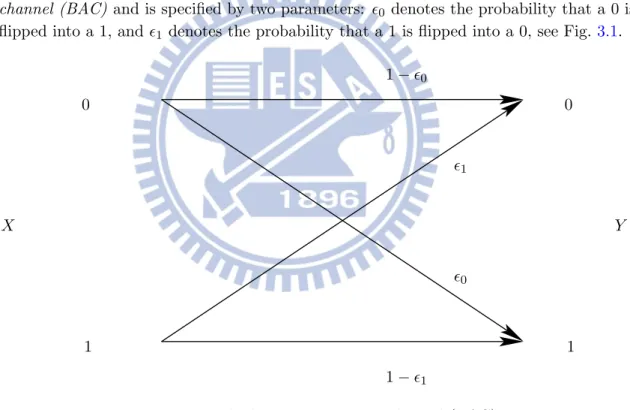
We consider a discrete memoryless channel (DMC) with both a binary input and a binary output alphabets. The most general such binary DMC is the so-called binary asymmetric channel (BAC) and is specified by two parameters: %0 denotes the probability that a 0 is flipped into a 1, and %1 denotes the probability that a 1 is flipped into a 0, see Fig.3.1.
0 0 1 1 %0 %1 1 − %0 1 − %1 X Y
Figure 3.1: The binary asymmetric channel (BAC).
For symmetry reasons and without loss of generality, we can restrict the values of these parameters as follows:
0 ≤ %0 ≤ %1 ≤ 1 (3.1) %0≤ 1 − %0 (3.2) %0≤ 1 − %1. (3.3) Note that in the case when %0 > %1, we simply flip all zeros to ones and vice versa to get
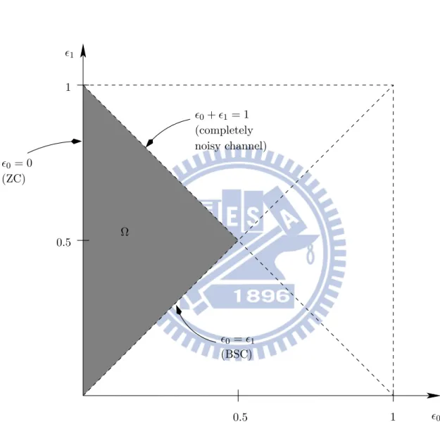
%0 %1 Ω %0+ %1= 1 (completely noisy channel) %0= %1 (BSC) %0 = 0 (ZC) 0.5 1 0.5 1
Figure 3.2: Region of possible choices of the channel parameters %0 and %1 of a BAC. The shaded area corresponds to the interesting area according to (3.1)–(3.3).
an equivalent channel with %0 ≤ %1. For the case when %0 > 1 − %0, we flip the output Y , i.e., change all output zeros to ones and ones to zeros, to get an equivalent channel with %0 ≤ 1 − %0. Note that (3.2) can be simplified to %0 ≤ 12 and is actually implied by (3.1) and (3.3). And for the case when %0 > 1 − %1, we flip the input X to get an equivalent channel that satisfies %0 ≤ 1 − %1.
We have depicted the region of possible choices of the parameters %0 and %1 in Fig.3.2. The region of interesting choices given by (3.1)–(3.3) is denoted by Ω.
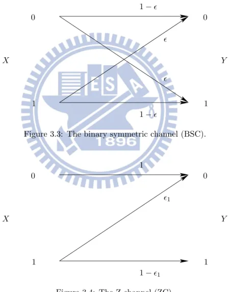
Note that the boundaries of Ω correspond to three special cases: The binary symmetric channel (BSC) (see Fig. 3.3) has equal cross-over probabilities %0 = %1 = %. According to (3.2), we can assume without loss of generality that % ≤ 12.
0 0 1 1 % % 1 − % 1 − % X Y
Figure 3.3: The binary symmetric channel (BSC).
0 0 1 1 1 %1 1 − %1 X Y
Figure 3.4: The Z-channel (ZC).
The Z-channel (ZC) (see Fig. 3.4) will never distort an input 0, i.e., %0 = 0. An input 1 is flipped to 0 with probability %1 < 1.
Finally, the case %0= 1−%1 corresponds to a completely noisy channel of zero capacity: given Y = y, the events X = 0 and X = 1 are equally likely, i.e., X ⊥⊥ Y .
A special case of the binary input and ternary output channel is BEC, which is not belong the special case of BAC, we have the transition probability, δ, from zero to one. The output alphabets of BEC are {0, 1, 2}, which is not binary. Here is the channel model defined as the following figure:
0 0 1 1 2 δ δ 1 − δ 1 − δ Figure 3.5: BEC
Due to the symmetry of the BSC and BEC, we have an additional equivalence in the codebook design.
Lemma 3.1 Consider an arbitrary code C(M,n) to be used on the BSC or BEC and con-sider an arbitrary M-vector c. Now construct a new length-(n + 1) code C(M,n+1) by appending c to the codebook matrix of C(M,n) and a new length-(n + 1) code C(M,n+1) by appending the flipped vector ¯c = c ⊕ 1 to the codebook matrix of C(M,n). Then the performance of these two new codes is identical:
Pe(n+1)"C(M,n+1)#= Pe(n+1),C(M,n+1)-. (3.4) We remind the reader that our ultimate goal is to find the structure of an optimal code C(M,n)∗ that satisfies
Pe(n)"C(M,n)∗#≤ P(n) e
"
C(M,n)# (3.5) for any code C(M,n).
Preliminaries
4.1
Error Probability of the BAC
The conditional probability of the received vector y given the sent codeword xm of the BAC can be written as
PYn|X(y|xm) = (1 − %0)d0,0(xm,y)· %d00,1(xm,y)· %
d1,0(xm,y)
1 · (1 − %1)d1,1(xm,y) (4.1) where we use Pn
Y|X to denote the product distribution PYn|X(y|x) = n ! j=1 PY|X(yj|xj). (4.2) Considering that n = d0,0(xm, y) + d0,1(xm, y) + d1,0(xm, y) + d1,1(xm, y) (4.3) the average error probability of a coding scheme C(M,n) over a BAC can now be written as Pe"C(M,n)#= 1 M M $ m=1 $ y g(y)&=m PYn|X(y|xm) (4.4) = (1 − %0) n M $ y M $ m=1 m&=g(y) . %0 1 − %0 /d0,1(xm,y) · . %1 1 − %0 /d1,0(xm,y). 1 − % 1 1 − %0 /d1,1(xm,y) (4.5) where g(y) is the ML decision (2.13) for the observation y.
4.1.1 Capacity of the BAC
Without loss of generality, we can only consider BACs with 0 ≤ %0 ≤ %1 ≤ 1 and 0 ≤ %0+ %1 ≤ 1.
Proposition 4.1 The capacity of a BAC is given by CBAC= %1 1 − %0− %1 · Hb(%0) − 1 − %0 1 − %0− %1 · Hb(%1) + log2 . 1 + 2Hb(!1)−Hb(!0)1−!0−!1 / (4.6) bits, where Hb(·) is the binary entropy function defined as
Hb(p) ! −p log2p − (1 − p) log2(1 − p). (4.7) The input distribution PX∗(·) that achieves this capacity is given by
PX∗(0) = 1 − PX∗(1) = z − %1(1 + z) (1 + z)(1 − %0− %1)
(4.8) with
z ! 2Hb(!1)−Hb(!0)1−!0−!1 . (4.9)
4.2
Error (and Success) Probability of the ZC
In the special case of a ZC, the average success probability can be expressed as follows: Pc"C(M,n)# = 1 M $ y M $ m=1 g(y)=m I{d01(xm, y) = 0} %d10(xm,y) 1 (1 − %1) d11(xm,y) (4.10) = 1 M $ y M $ m=1 g(y)=m I{d0,1(xm, y) = 0} . %1 1 − %1 /d1,0(xm,y) · (1 − %1)d1,1(xm,y)+d1,0(xm,y)(4.11) = 1 M M $ m=1 $ y g(y)=m I{d0,1(xm, y) = 0} . %1 1 − %1 /d1,0(xm,y) · (1 − %1)wH(xm). (4.12) The error probability formula is accordingly
Pe"C(M,n)#= 1 M M $ m=1 $ y g(y)&=m I{d0,1(xm, y) = 0} · . %1 1 − %1 /d1,0(xm,y) (1 − %1)wH(xm). (4.13) From (B.52), note that the capacity-achieving distribution for %1= 12 is
PX∗(1) = 2
5. (4.14) The capacity-achieving distribution is strongly depends on the cross-over probability %1.
4.3
Error (and Success) Probability of the BSC
In the special case of a BSC, (4.5) simplifies to Pe " C(M,n)#= (1 − %) n M $ y M $ m=1 g(y)&=m . % 1 − % /dH(xm,y) . (4.15) The success probability is accordingly
Pc"C(M,n)#= (1 − %) n M $ y M $ m=1 g(y)=m . % 1 − % /dH(xm,y) . (4.16) 4.3.1 Capacity of the BSC
From (C.97), the capacity of a BSC is given by
CBSC = 1 − Hb(%) (4.17) bits. The input distribution PX∗(·) that achieve the capacity is the uniform distribution given by
PX∗(0) = 1 − PX∗(1) = 1
2, (4.18) which is irrelevant to the cross-over prbability %.
4.4
Error (and Success) Probability of the BEC
The only difference of BEC is the output turn out to be ternary.
Definition 4.2 To make the conditional probability express shortly, we defined the number of times the symbol a occurs in one received vector y by N(a|y). By I(a|y) we denote the set of indices i such that yi= a, hence N(a|y) = |I(a|y)|, i.e., xI(a|y) is a vector of length N(a|y) containing all xi where i ∈ I(a|y).
It is often easier to maximize the success probability instead of minimizing the error probability. For the convenience of later derivations, we are going to derive its error and success probabilities: Pc(C(M,n)) = 1 M M $ m=1 $ y g(y)=m (1 − %)n−N(2|y)· %N(2|y) ·I0dH"xm I(b|y), yI(b|y)
#
where b ∈ {0, 1}. The error probability formula is accordingly Pe(C(M,n)) = 1 M M $ m=1 $ y g(y)&=m (1 − %)n−N(2|y)· %N(2|y) ·I0dH " xm I(b|y), yI(b|y) # = 01 (4.20)
4.4.1 Capacity of the BEC
The capacity of a BEC is given by
CBEC= 1 − δ (4.21) bits. The input distribution PX∗(·) that achieve the capacity is the uniform distribution given by
PX∗(0) = 1 − PX∗(1) = 1
2, (4.22) which is also irrelevant to the cross-over probability δ.
4.5
Pairwise Hamming Distance
The minimum Hamming distance is a well-known and often used quality criterion of a codebook [12], [13]. [13, Ch. 2] discusses the maximum minimum Hamming distance for a given code C(M,n), e.g., the Plotkin bound and Levenshtein’s theorem. (For discussions of the upper and lower bounds to average error probability, see Chapter7.) Unfortunately, a design based on the minimum Hamming distance can fail even for linear codes and even for a very symmetric channel like the BSC, whose error probability performance is completely specified by the Hamming distances between codewords and received vectors.
We therefore define a slightly more general and more concise description of a codebook: the pairwise Hamming distance vector.
Definition 4.3 Given a codebook C(M,n) with codewords xm, 1 ≤ m ≤ M, we define the length 12(M − 1)M pairwise Hamming distance vector
d"C(M,n)# !,dH(x1, x2), dH(x1, x3), dH(x2, x3), dH(x1, x4), dH(x2, x4), dH(x3, x4), . . . , dH(x1, xM), dH(x2, xM), . . . , dH(xM−1, xM) -. (4.23) The minimum Hamming distance dmin"C(M,n)#is then defined as the minimum component of the pairwise Hamming distance vector d"C(M,n)#.
A Counterexample
To show that the search for an optimal (possibly nonlinear) code is neither trivial nor intuitive even in the symmetric BSC case, we would like to start with a simple example before we summarize our main results.
Assume a BSC with cross probability % = 0.4, M = 4, and a blocklength n = 4. Then consider the following codes:4
C(4,4) 1 = 0 0 0 0 0 0 0 1 1 1 1 0 1 1 1 1 , C(4,4) 2 = 0 0 0 0 0 0 1 1 1 1 0 0 1 1 1 1 . (5.1) We observe that while both codes are linear (i.e., any sum of two codewords is also a codeword), the first code has a minimum Hamming distance 1, and the second has a minimum Hamming distance 2. It is quite common to believe that C2(4,4) shows a better performance. This intuition is based on Gallager’s famous performance bound [6, Exercise 5.19]: Pe " C(M,n)#≤ (M − 1)e−dmin(C (M,n)) log√ 1 4!(1−!). (5.2)
However, the exact average error probability as given in (4.15) actually can be evaluated as Pe"C1(4,4)
#
≈ 0.6112 and Pe"C2(4,4) #
= 0.64. Hence, even though the minimum Hamming distance of the first codebook is smaller, its overall performance is superior to the second codebook!
Our goal is to find the structure of an optimal code C(M,n)∗ that satisfies Pe
"
C(M,n)∗#≤ Pe"C(M,n)# (5.3) for any code C(M,n).
4We will see in Chapter 6that both codes are weak flip codes. In this example, C(4,4)
1 = C
(4,4) 1,0 and
Flip Codes, Weak Flip Codes and
Hadamard Codes
We next introduce some special families of binary codes. We start with a family of codes with two codewords.
Definition 6.1 The flip code of type t for t ∈ 00, 1, . . . ,2n231 is a code with M = 2 codewords defined by the following codebook matrix Ct(2,n):
tcolumns 4 56 7 C(2,n) t ! 8 x ¯ x 9 = 8 0 · · · 0 1 · · · 1 1 · · · 1 0 · · · 0 9 . (6.1) Defining the column vectors
% c(2)1 ! 8 0 1 9 , c(2)2 ! 8 1 0 9: , (6.2) we see that a flip code of type t is given by a codebook matrix that consists of n − t columns c(2)1 and t columns c(2)2 .
We again remind the reader that due to the memorylessness of the BEC, other codes with the same columns as Ct(2,n), but in different order are equivalent to Ct(2,n). Moreover, we would like to point out that while the flip code of type 0 corresponds to a repetition code, the general flip code of type t with t > 0 is neither a repetition code nor is it even linear. We have shown in [16] that for any blocklength n and for a correct choice5 of t, the flip codes are optimal on any binary-input binary-output channel for arbitrary channel parameters. In particular, they are optimal for the BSC and the ZC [16].
The columns given in the set in (6.2) are called candidate columns. They are flipped versions of each other, therefore also the name of the code.
5We would like to emphasize that the optimal choice of t for many binary channels is not 0, i.e., the
The definition of a flip code with one codeword being the flipped version of the other cannot be easily extended to a situation with more than two codewords. Hence, for M > 2, we need a new approach. We give the following definition.
Definition 6.2 Given an M > 2, a length-M candidate column c is called a weak flip column if its first component is 0 and its Hamming weight equals to 2M
2 3 or ;M 2 < . The collection of all possible weak flip columns is called weak flip candidate columns set and is denoted by C(M).
We see that a weak flip column contains an almost equal number of zeros and ones. The restriction of the first component to be zero is based on the insight of Lemma 3.1. For the remainder of this work, we introduce the shorthand
' ! =M
2 >
. (6.3)
Lemma 6.3 The cardinality of a weak flip candidate columns set is ?
?C(M)??=.2' − 1 '
/
. (6.4)
Proof: If M = 2', then we have "2#−1# # possible choices, while if M = 2' − 1, we have "2#−2#−1#+"2#−2# #="2#−1# # choices.
We are now ready to generalize Definition 6.1.
Definition 6.4 A weak flip code is a codebook that is constructed only by weak flip columns.
Concretely, for M = 3 or M = 4, we have the following.
Definition 6.5 The weak flip code of type (t2, t3) for M = 3 or M = 4 codewords is defined by a codebook matrix Ct(M,n)2,t3 that consists of t1 ! n − t2 − t3 columns c(M)1 , t2 columns c(M)2 , and t3 columns c(M)3 , where
c(3)1 ! 0 0 1 , c (3) 2 ! 0 1 0 , c (3) 3 ! 0 1 1 (6.5) or c(4)1 ! 0 0 1 1 , c(4)2 ! 0 1 0 1 , c(4)3 ! 0 1 1 0 , (6.6) respectively. We often describe the weak flip code of type (t2, t3) by its code parameters
where t1 can be computed from the blocklength n and the type (t2, t3) as t1 = n − t2− t3. Moreover, we use
D(M,n)t2,t3;m! {y : g(y) = m} (6.8) to denote the decoding region of the mth codeword of Ct(M,n)2,t3 .
An interesting subfamily of weak flip codes of type (t2, t3) for M = 3 or M = 4 is defined as follows.
Definition 6.6 A fair weak flip code of type (t2, t3), Ct(M,n)2,t3 , with M = 3 or M = 4
codewords satisfies that
t1 = t2 = t3. (6.9) Note that the fair weak flip code of type (t2, t3) is only defined provided that the block-length satisfies n mod 3 = 0. In order to be able to provide convenient comparisons for every blocklength n, we define a generalized fair weak flip code for every n, C(M,n)
,n+1 3 -,, n 3 -, where t2 =G n + 1 3 H , t3 =I n 3 J . (6.10) If n mod 3 = 0, the generalized fair weak flip code actually is a fair weak flip code.
The following lemma follows from the respective definitions in a straightforward man-ner. We therefore omit its proof.
Lemma 6.7 The pairwise Hamming distance vector of a weak flip code of type (t2, t3) can be computed as follows:
d(3,n) = (t2+ t3, t1+ t3, t1+ t2),
d(4,n) = (t2+ t3, t1+ t3, t1+ t2, t1+ t2, t1+ t3, t2+ t3).
A similar definition can be given also for larger M, however, one needs to be aware that the number of weak flip candidate columns is increasing fast. For M = 5 or M = 6 we have ten weak flip candidate columns:
c(5)1 ! 0 0 0 1 1 , c(5)2 ! 0 0 1 0 1 , c(5)3 ! 0 0 1 1 0 , c(5)4 ! 0 0 1 1 1 , c(5)5 ! 0 1 0 0 1 , c(5)6 ! 0 1 0 1 0 , c(5)7 ! 0 1 0 1 1 ,
c(5)8 ! 0 1 1 0 0 , c(5)9 ! 0 1 1 0 1 , c(5)10 ! 0 1 1 1 0 , (6.11) and c(6)1 ! 0 0 0 1 1 1 , c(6)2 ! 0 0 1 0 1 1 , c(6)3 ! 0 0 1 1 0 1 , c(6)4 ! 0 0 1 1 1 0 , c(6)5 ! 0 1 0 0 1 1 , c(6)6 ! 0 1 0 1 0 1 , c(6)7 ! 0 1 0 1 1 0 , c(6)8 ! 0 1 1 0 0 1 , c(6)9 ! 0 1 1 0 1 0 , c(6)10 ! 0 1 1 1 0 0 , (6.12) respectively.
We will next introduce a generalized fair weak flip codes, as we will see in Section6.1, possess particularly beautiful properties.
Definition 6.8 A weak flip code is called fair if it is constructed by an equal number of all possible weak flip candidate columns in C(M). Note that by definition the blocklength of a fair weak flip code is always a multiple of "2#−1# #, ' ≥ 2.
Fair weak flip codes have been used by Shannon et al. [17] for the derivation of error exponents, although the codes were not named at that time. Note that the error exponents are defined when the blocklength n goes to infinity, but in this work we consider finite n. Related to the weak flip codes and the fair weak flip codes are the families of Hadamard codes [13, Ch. 2].
Definition 6.9 For an even integer n, a ( normalized) Hadamard matrix Hn of order n is an n × n matrix with entries +1 and −1 and with the first row and column being all +1, such that
if such a matrix exists. Here In is the identity matrix of size n. If the entries +1 are replaced by 0 and the entries −1 by 1, Hn is changed into the binary Hadamard matrix An.
Note that a necessary (but not sufficient) condition for the existence of Hn (and the corresponding An) is that n is a 1, 2 or multiple of 4 [13, Ch. 2].
Definition 6.10 The binary Hadamard matrix Angives rise to three families of Hadamard codes:
1. The "n, n − 1,n 2 #
Hadamard code H1,n consists of the rows of An with the first column deleted. The codewords in H1,n that begin with 0 form the "n2, n − 2,n2# Hadamard code H1,n$ if the initial zero is deleted.
2. The "2n, n − 1,n 2 − 1
#
Hadamard code H2,n consists of H1,n together with the com-plements of all its codewords.
3. The "2n, n,n 2 #
Hadamard code H3,n consists of the rows of An and their comple-ments.
Further Hadamard codes can be created by an arbitrary combinations of the codebook ma-trices of different Hadamard codes.
Example 6.11 Consider a (6, 10, 6) H$ 1,12 code: 0 0 0 0 0 0 0 0 0 0 0 0 0 0 1 1 1 1 1 1 0 1 1 1 0 0 0 1 1 1 1 0 1 1 0 1 1 0 0 1 1 1 0 1 1 0 1 0 1 0 1 1 1 0 1 1 0 1 0 0 (6.14)
From this code, see the candidate columns (6.12) for M = 6, it is identical to the fair weak flip code for M = 6. Since the fair weak flip code already used up all the possible weak flip candidate columns, hence, there is only one (6, 10, 6) H1,12$ in column-wise respect. Example 6.12 Consider an (8, 7, 4) H1,8 code:
H1 1,8 = 0 0 0 0 0 0 0 0 0 1 0 1 1 1 0 1 0 1 0 1 1 0 1 1 1 1 0 0 1 0 0 1 1 0 1 1 0 1 1 0 1 0 1 1 0 0 1 1 0 1 1 1 0 0 0 1 , (6.15)
and the other (8, 7, 4) H2 1,8 code: H1,82 = 0 0 0 0 0 0 0 0 0 1 0 1 1 1 1 0 0 1 1 0 1 0 1 1 1 1 0 0 1 1 1 0 0 0 1 1 0 1 1 0 1 0 0 1 0 1 0 1 1 1 1 0 0 1 1 0 . (6.16)
From these codes, an (8, 35, 20) Hadamard code can be constructed by simply concatenating H1
1,8 five times, or concatenating H1,81 three times and H1,82 two times.
Note that since the rows of Hn are orthogonal, any two rows of An agree in 12n places and differ in 12n places, i.e., they have a Hamming distance 12n. Moreover, by definition the first row of a binary Hadamard matrix is the all-zero row. Hence, we see that all Hadamard codes are weak flip codes, i.e., the family of weak flip codes is a superset of Hadamard codes.
On the other hand, every Hadamard code of parameters (M, n), for which fair weak flip codes exist, is not necessarily equivalent to a fair weak flip code. We also would like to remark that the Hadamard codes rely on the existence of Hadamard matrices. So in general, it is very difficult to predict whether for a given pair (M, n), a Hadamard code will exist or not. This is in stark contrast to weak flip codes (which exist for all M and n) and fair weak flip codes (which exist for all M and all n being a multiple of "2#−1# #). Example 6.13 We continue with Example 6.12 and note that the (8, 35, 20) Hadamard code that is constructed by five repetitions of the matrix given in (6.15) is actually not a fair weak flip code, since we have to use up all possible weak flip candidate columns to get a (8, 35, 20) fair weak flip code.
Note that two Hadamard matrices can be equivalent if one can be obtained from the other by permuting rows and columns and multiplying rows and columns by −1. In other words, Hadamard codes can actually be constructed from weak candidate columns. This also follows directly from the already mentioned fact that Hadamard codes are weak flip codes.
6.1
Characteristics of Weak Flip Codes
In conventional coding theory, most results are restricted to so called linear codes that possess very powerful algebraic properties. For the following definitions and proofs see, e.g., [12], [13].
Definition 6.14 Let M = 2k, where k ∈ N. The binary code C(M,n)
lin is linear if its codewords span a k-dimensional subspace of {0, 1}n.
One of the most important property of a linear code is as follows.
Proposition 6.15 Let Clin be linear and let xm ∈ Clin be given. Then the code that we obtain by adding xm to each codeword of Clin is equal to Clin.
Another property concerns the column weights.
Proposition 6.16 If an (M, n) binary code is linear, then each column of its codebook matrix has Hamming weight M2, i.e., the code is a weak flip code.
Hence, linear codes are weak flip codes. Note, however, that linear codes only exist if M = 2k, where k ∈ N, while weak flip codes are defined for any M. Also note that the converse of Proposition 6.16 does not hold, i.e., even if M = 2k for some k ∈ N, a weak flip code C(M,n) is not necessarily linear. It is not even the case that a fair weak flip code for M = 2k is necessarily linear!
Now the question arises as to which of the many powerful algebraic properties of linear codes are retained in weak flip codes.
Theorem 6.17 Consider a weak flip code C(M,n) and fix some codeword xm ∈ C(M,n). If we add this codeword to all codewords in C(M,n), then the resulting code ˜C(M,n) ! 0
xm ⊕ x ?
?∀ x ∈ C(M,n)1 is still a weak flip code, however, it is not necessarily the same one.
Proof: Let C(M,n) be according to Definition6.4. We have to prove that x1 x2 .. . xM ⊕ xm xm .. . xm = x1⊕ xm .. . xm⊕ xm= 0 .. . xM⊕ xm ! ˜C(M,n) (6.17)
is a weak flip code. Let ci denote the column vectors of C(M,n). Then ˜C(M,n) has the column vectors ˜ ci= % ci if xm,i= 0, ¯ ci if xm,i= 1, (6.18) for 1 ≤ i ≤ n. Since ci is a weak flip column, either wH(ci) = 2M23 and therefore wH(¯ci) = ;M 2 < , or wH(ci) = ;M 2 < and therefore wH(¯ci) = 2M 2 3 . So we only need to interchange the first codeword of ˜C and the all-zero codeword in the mth row in ˜C (which is always possible, see discussion after Definition 2.7), and we see that ˜C is also a weak flip code.
Theorem 6.17 is a beautiful property of weak flip codes; however, it still represents a considerable weakening of the powerful property of linear codes given in Proposition6.15. This can be fixed by considering the subfamily of fair weak flip codes.
Theorem 6.18 (Quasi-Linear Codes) Let C be a fair weak flip code and let xm ∈ C be given. Then the code ˜C =0xm⊕ x??∀ x ∈ C(M,n)1is equivalent to C .
Proof: We have already seen in Theorem6.17that adding a codeword will result in a weak flip code again. In the case of a fair weak flip code, however, all possible candidate columns will show up again with the same equal frequency. It only remains to rearrange some rows and columns.
If we recall Proposition 6.16and the discussion after it, we realize that the definition of the quasi-linear fair weak flip code is a considerable enlargement of the set of codes having the property given in Theorem 6.18.
The following corollary is a direct consequence of Theorem 6.18.
Corollary 6.19 The Hamming weights of each codeword of a fair weak flip code are all identical except the all-zero codeword x1. In other words, if we let wH(·) be the Hamming weight function, then
wH(x2) = wH(x3) = · · · = wH(xM). (6.19) Before we next investigate the minimum Hamming distance for the quasi-linear fair weak flip codes, we quickly recall an important bound that holds for any "M, n, d# code. Lemma 6.20 (Plotkin Bound [13]) The minimum distance of an (M, n) binary code C(M,n) always satisfies dmin"C(M,n)#≤ n·M 2 M−1 Meven, n·M+1 2 M Modd. (6.20) Proof: We show a quick proof. We sum the Hamming distance over all possible pairs of two codewords apart from the codeword with itself:
M(M − 1) · dmin(C(M,n)) ≤ $ u∈C(M,n) $ v∈C(M,n) v&=u dH(u, v) (6.21) = n $ j=1 2bj· (M − bj) (6.22) ≤ % n · M2 2 if M even (achieved if bj = M/2), n · M2−1 2 if M odd (achieved if bj = (M ± 1)/2). (6.23) Here in (A.33) we rearrange the order of summation: instead of summing over all code-words (rows), we approach the problem column-wise and assume that the jth column of C(M,n) contains bj zeros and M − bj ones: then this column contributes 2bj(M − bj) to the sum.
Note that from the proof of Lemma 6.20 we can see that a necessary condition for a codebook to meet the Plotkin-bound is that the codebook is composed by weak flip
candidate columns. Furthermore, Levenshtein [13, Ch. 2] proved that the Plotkin bound can be achieved, provided that Hadamard matrices exist.
Theorem 6.21 Fix some M and a blocklength n with n mod"2#−1# # = 0. Then a fair weak flip code C(M,n) achieves the largest minimum Hamming distance among all codes of given blocklength and satisfies
dmin "
C(M,n)#= n · '
2' − 1. (6.24) Proof: For M = 2', we know that by definition the Hamming weight of each column of the codebook matrix is equal to '. Hence, when changing the sum from column-wise to row-wise, where we can ignore the first row of zero weight (from the all-zero codeword x1), we get n · ' = n $ j=1 wH(cj) = 2# $ m=2 wH(xm) (6.25) = 2# $ m=2 dmin " C(M,n)# (6.26) = (2' − 1) · dmin"C(M,n)#. (6.27) Here, (B.42) follows from Theorem 6.18 and from Corollary 6.19. For M = 2' − 1, the Hamming distance remains the same due to the fair construction.
It remains to show that a fair weak flip code achieves the largest minimum Hamming distance among all codes of given blocklength. From Corollary 6.19we know that (apart from the all-zero codeword) all codewords of a fair weak flip code have the same Hamming weight. So, if we flip an arbitrary 1 in the codebook matrix to become a 0, then the corresponding codeword has a decreased Hamming weight and is therefore closer to the all-zero codeword. If we flip an arbitrary 0 to become a 1, then the corresponding codeword is closer to some other codeword that already has a 1 in this position. Hence, in both cases we have reduced the minimum Hamming distance. Finally, based on the concept of looking at the code in column-wise, it can be seen that whenever we change more than one bit, we either get back to a fair weak flip code or to another code who is worse.
Previous Work
7.1
SGB Bounds on the Average Error Probability
In [17], Shannon, Gallager, and Berlekamp derive upper and lower bounds on the average error probability of a given code used on a DMC. We next quickly review their results. Definition 7.1 For 0 < s < 1 we define
µα,β(s) ! ln $
y
PY|X(y|α)1−sPY|X(y|β)s. (7.1) Therefore, the generalized µ(s) for blocklength n between xm and xm" can be defined and
expressed in terms of (7.1) by µ(s) ! ln$ y PY|X(y|xm)1−sPY|X(y|xm")s= n $ α $ β qα,β(m, m$)µα,β(s), (7.2) and the discrepancy D(DMC)(m, m$) between xm and xm" is defined as
D(DMC)(m, m$) ! − min 0≤s≤1 $ α $ β qα,β(m, m$)µα,β(s) (7.3) with qα,β(m, m$) given in Def.2.9.
Note that the discrepancy is a generalization of the Hamming distance, however, it depends strongly on the channel cross-over probabilities. We use a superscript “(DMC)” to indicate the channel which the discrepancy refers to.
Definition 7.2 The minimum discrepancy D(DMC)min (C(M,n)) for a codebook is the mini-mum value of D(DMC)(m, m$) over all pairs of codewords. The maximum minimum dis-crepancy is the maximum value of D(DMC)min (C(M,n)) over all possible C(M,n) codebooks: maxC(M,n)D(DMC)min (C(M,n)).
Theorem 7.3 (Lower Bounds to Conditional Error Probability [17]) If xm and xm" are pair of codewords in a code of blocklength n, then either
λm > 1 4exp −n K D(DMC)(m, m$) + L 2 nln (1/Pmin) M (7.4) or λm" > 1 4exp −n K D(DMC)(m, m$) + L 2 nln (1/Pmin) M , (7.5) where Pmin is the smallest nonzero transition probability for the channel.
Conversely, one can also show that λm ≤ (M − 1) exp −n , D(DMC) min " C(M,n)#-, for all m. (7.6) Theorem 7.4 (SGB Bounds on Average Error Probability [17]) For an arbitrary DMC, the average error probability Pe"C(M,n)# of a given code C(M,n) with M codewords and blocklength n is upper- and lower-bounded as follows:
1 4Me −n!D(DMC) min (C(M,n))+ " 2 nlog 1 Pmin # ≤ Pe"C(M,n)#≤ (M − 1)e−nD (DMC) min (C(M,n)) (7.7)
where Pmin denotes the smallest nonzero transition probability of the channel.
Note that these bounds are specific to a given code design (via D(DMC)min ). Therefore, the upper bound is a generally valid upper bound on the optimal performance, while the lower bound only holds in general if we apply it to the optimal code or to a suboptimal code that achieves the optimal Dmin.
The bounds (7.7) are tight enough to derive the error exponent of the DMC (for a fixed number M of codewords).
Theorem 7.5 ([17]) The error exponent of a DMC for a fixed number M of codewords EM ! lim n→∞Cmax(M,n) N −1 nlog Pe " C(M,n)# O (7.8) is given as EM= lim n→∞Cmax(M,n) D(DMC) min " C(M,n)#. (7.9) Unfortunately, in general the evaluation of the error exponent is very difficult. For some cases, however, it can be done. For example, for M = 2, we have
E2 = max C(2,n) D(DMC) min " C(2,n)#= max α,β N − min 0≤s≤1µα,β(s) O . (7.10) Also for the class of so-called pairwise reversible channels, the calculation of the error exponent turns out to be uncomplicated.
Definition 7.6 A pairwise reversible channel is a DMC that has µ$
α,β(12) = 0 for any inputs α, β.
Clearly, the BSC and BEC are pairwise reversible channels.
Note that it is easy to compute the pairwise discrepancy of a linear code on a pairwise reversible channel, so linear codes are quite suitable for computing (7.7).
Theorem 7.7 ([17]) For pairwise reversible channels with M > 2, EM = 1 M(M − 1) Mmaxxs.t. $ xMx=M $ all input letters x $ all input letters x" MxMx" · 8 − ln$ y P PY|X(y|x)PY|X(y|x$) 9 (7.11) where Mx denotes the number of times the channel input letter x occurs in a column. Moreover, EM is achieved by fair weak flip codes.6
We would like to emphasize that while Shannon et al. proved that fair weak flip codes achieve the error exponent, they did not investigate the error performance of fair weak flip codes for finite n. As we will show later, fair weak flip might be strictly suboptimal codes for finite n (see also [18]).
7.2
Gallager Bound
Another famous bound is by Gallager [6].
Theorem 7.8 ([6]) For an arbitrary DMC, there exists a code C(M,n) with M = 2enR3 such that
Pe"C(M,n)#≤ e−nEG(R) (7.12) where EG(·) is the Gallager exponent and is given by
EG(R) = max Q(·) 0≤ρ≤1max 0 E0(ρ, Q) − ρR1 (7.13) with E0(ρ, Q) ! −log $ y 8 $ x Q(x)PY|X(y|x) 1 1+ρ 91+ρ . (7.14)
6While throughout we only consider binary inputs and M = 3 or M = 4, the definitions of our fair
weak flip codes can be generalized to nonbinary inputs and larger M. Also these generalized fair weak flip codes will achieve the corresponding error exponents. Note that Shannon et al. did not actually name their exponent-achieving codes.
7.3
PPV Bounds for the BSC
In [2], Polyanskiy, Poor, and Verd´u present upper and lower bounds on the optimal average error probability for finite blocklength for the BSC. The upper bound is based on random coding.
Theorem 7.9 (PPV Upper Bound [19, Theorem 2], [2, Theorem 32]) If the code-book C(M,n)is created at random based on a uniform distribution, the expected average error probability (averaged over all codewords and all codebooks) satisfies
EQPe"C(M,n)#R= 1 − 2n−nM n $ i=0 .n i / %i(1 − %)n−i · M−1 $ m=0 1 m + 1 .M − 1 m /.n i /m n $ j=i+1 .n j / M−1−m . (7.15) Note that there must exist a codebook whose average error probability achieves (7.15), so Theorem 7.9provides a general achievable upper bound, although we do not know its concrete code structure.
Polyanskiy, Poor, and Verd´u also provide a new general converse for the average error probability: the so-called meta-converse, which is based on binary hypothesis testing. For a BSC, the meta-converse lower bound happens to be equivalent to Gallager’s sphere-packing bound.
Theorem 7.10 (PPV Lower Bound [6, p. 163, Eq. (5.8.19)], [2, Theorem 35]) Any codebook C(M,n) satisfies Pe"C(M,n)#≥ 8. n N / − 1 M M $ m=1 Am,N 9 %N(1 − %)n−N + n $ j=N+1 .n j / %j(1 − %)n−j (7.16) where for m ∈ {1, . . . , M} and for j ∈ {1, . . . , N − 1, N + 1, . . . , n}
Am,j = "n j # 0 ≤ j ≤ N − 1 0 N+ 1 ≤ j ≤ n (7.17) and where the positive integer N and coefficients Am,N are chosen such that
M N−1 $ j=0 Am,j+ M $ m=1 Am,N= 2n (7.18) 0 < M $ m=1 Am,N≤ M. n N / . (7.19)
7.4
PPV Bounds for the BEC
In [2], Polyanskiy, Poor, and Verd´u present upper and lower bounds on the optimal average error probability for finite blocklength for the BEC. The upper bound is based on random coding.
Theorem 7.11 For the BEC with crossover probability δ, the average error probability for an random code is given by
ESPe"C(M,n)#T = 1 − n $ j=0 .n j / (1 − δ)jδn−j M−1 $ #=0 1 ' + 1 .M − 1 ' / (2−j)#(1 − 2−j)M−1−#. (7.20) Note that there must exist a codebook whose average error probability achieves (C.16), so Theorem 7.11provides a general achievable upper bound, although we do not know its concrete code structure.
Polyanskiy, Poor, and Verd´u also provide a new general converse for the average error probability for a BEC.
Theorem 7.12 For the BEC with erasure probability δ, the average error probability of a C(M,n) code satisfies Pe"C(M,n)#≥ n $ #=*n−log2M++1 .n ' / δ#(1 − δ)n−# . 1 −2 n−# M / . (7.21) Note that this lower bound is not derived by the method: meta-converse, it is from other technique.
Analysis of the BAC
We start with results that hold for the general BAC. In this section we will restrict ourselves to two codewords M = 2. One can show that the BAC is a pairwise reversible channel, however, in this analysis we do not focus on its bounds on its performance, but put a special emphasis on the optimal code design.
8.1
Optimal Codes
Theorem 8.1 Consider a BAC and a blocklength n. Then, irrespective of the channel parameters %0 and %1, there exists a choice of t, 0 ≤ t ≤ 2n23, such that the flip code of type t, Ct(2,n), is optimal in the sense that it minimizes the average error probability.
Proof: Consider an arbitrary code with M = 2 codewords and a blocklength n + j, and assume that this code is not a flip code, but that it has a number j of positions where both codewords have the same symbol. An optimal decoder will ignore these j positions completely. Hence, the performance of this code will be identical to a flip code of length n. Now, change this code in the j positions with identical symbol such that the code becomes a flip code. If we use a suboptimal decoder that ignores these j positions we still keep the same performance. However, an ML decoder can potentially improve the performance, i.e., we have
Pe"Cnot flip(M,n+j)#ML decoder = Pe"Cflip(M,n+j)#suboptimal decoder (8.1) ≥ Pe"Cflip(M,n+j)#ML decoder. (8.2) An alternative proof is shown in Appendix A.3. While this proof is more elaborate, it turns out to be very useful for the derivation of Theorem 8.3.
This result is intuitively very pleasing because it seems to be a rather bad choice to have two codewords with the same symbol in a particular position, i.e., x1,j = x2,j = 0 in the same position j. However, note that the theorem does not exclude the possibility that another code might exist that also is optimal and that has an identical symbol in both codewords at a given position.
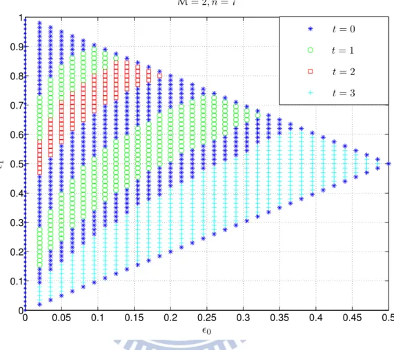
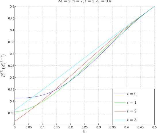
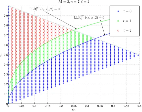
We would like to point out that the exact choice of t is not obvious and depends strongly on n, %0, and %1. As an example, the optimal choices of t are shown in Fig.8.6for n = 7. We see that depending on the channel parameters, the optimal value of t changes.
0 0.05 0.1 0.15 0.2 0.25 0.3 0.35 0.4 0.45 0.5 0 0.1 0.2 0.3 0.4 0.5 0.6 0.7 0.8 0.9 1 M= 2, n = 7 t = 0 t = 1 t = 2 t = 3 %0 %1
Figure 8.6: Optimal codebooks on a BAC: the optimal choice of the parameter t for different values of %0 and %1 for a fixed blocklength n = 7.
Note that for a completely noisy channel (%1 = 1 − %0), the choice of t is irrelevant since the probability of error is 12 for any code. Moreover, in Theorem9.1it will be shown that the flip codes of type 0 is optimal on the ZC; and in Theorem 10.1 it will be shown that the flip codes are optimal on the BSC for any choice of t. We defer the exact treatment of the ZC and the BSC to Chapter 9and 10, respectively.
8.2
The Optimal Decision Rule for Flip Codes
Having only two codewords, the ML decision rule can be expressed using the log-likelihood ratio (LLR). For the flip code of type t, Ct(2,n) (see Def. 6.1), the LLR is given as
log 8 Pn Y|X(y|x1) Pn Y|X(y|x2) 9