國 立 交 通 大 學
電子工程學系 電子研究所碩士班
碩 士 論 文
以統計分佈距離為基礎之感知無線電合作式頻譜偵測
技術
Distribution Distance based Collaborative Spectrum
Detection in Cognitive Radio Networks
研 究 生 : 陳信宏
指導教授 : 簡鳳村 博士
以統計分佈距離為基礎之感知無線電合作式頻譜偵測
技術
Distribution Distance based Collaborative Spectrum
Detection in Cognitive Radio Networks
研 究 生 : 陳信宏
Student: Shin-Horng Chen
指導教授 : 簡鳳村 博士
Advisor: Dr. Feng-Tsun Chien
國 立 交 通 大 學
電子工程學系 電子研究所碩士班
碩士論文
A Thesis
Submitted to Department of Electronics Engineering & Institute of Electronics College of Electrical and Computer Engineering
National Chiao Tung University in Partial Fulfillment of the Requirements
for the Degree of Master of Science
in
Electronics Engineering August 2009
Hsinchu, Taiwan, Republic of China
以統計距離分布為基礎之感知無線電合作式頻譜偵測
技術
研究生: 陳信宏 指導教授:簡鳳村博士
國立交通大學電子工程學系 電子研究所碩士班
摘要
在此論文中,我們討論了在感知無線電的環境中,使用了距離量測 (Distance measure)在機率分佈下之頻譜感測。使用距離量測當作效能之度量的原因是基於我們並不能輕易的從 log likelihood ratio 中得到近似解。所以在每一個次要使用 者 (Secondary users)中,我們採用距離量測作為度量。
這篇論文主要分為兩部分。在第一部分中,我們考慮集中式偵測的方式:每 一個次要使用者傳送沒有量化過的訊號到共同接收器 (Fusion center)來偵測是否 有頻譜洞 (Spectrum hole)存在。在此,我們使用兩種距離量測方法,J-divergence 及 L2 distance 來設計決策方法(Decision rule)。實際上,我們嘗試使用最佳功率 分配(Optimal power allocation)及最佳線性組合(Optimal linear combination)兩種方 法使偵測頻譜洞之偵測機率最大同時維持主要使用者收到的干擾在一定的程度 之內。從模擬結果可以看出,使用距離量測下所得到的偵測機率的確比相同功率 分布(Equal power allocation)及相同加權組合(Equal weighting combination)來的 好。
在第二部分中,我們考慮了使用設限(Censoring)之非集中式偵測。設限代表 了次要使用者只傳有資訊的資料到共同接收器,否則便不傳任何資料。因為高斯
混合模型(Gaussian mixture model)的關係,依然很難最大化偵測機率。所以我們 一樣使用距離量測的方式當作效能之度量。從模擬結果中我們可以看到,在設限 方法下的偵測機率,的確比原本沒有任何限制的方法還好。
Distribution Distance based Collaborative Spectrum
Detection in Cognitive Radio Networks
Student: Shin-Horng Chen
Advisor: Dr. Feng-Tsun Chien
Department of Electronics Engineering
Institute of Electronics
National Chiao Tung University
Abstract
In this thesis, we discuss the problem of collaborative spectrum sensing in
cognitive radio networks from the perspective of distance measures between
probability distributions. The rationale behind using the distance measures as the
performance metric lies on the difficulty of having a closed-form expression for the
log likelihood ratio. We adopt the distance measure as the metric to design the
decision criterion in each of the secondary users in the cooperative environment.
The thesis is mainly consisted of two parts. In the first part, we consider the case
of centralized detection in which every secondary user sends un-quantized signal to
the fusion center for the ultimate detection of the spectrum hole. We use two distance
measures, J-divergence and L2 distance, to design the local decision rule. In particular,
we attempt to devise a power allocation scheme among secondary users, as well as a
combination scheme to gather received signals in the fusion center, for maximizing
the probability of detection of a spectrum hole while keeping the interference
simulated results show that we can improve the detection probability by optimizing
the distance measures as compared to the equal power allocation and equal weight
combination.
In the second part, we consider the case of decentralized detection with censoring.
The censoring means the secondary users only transmit informative observations to
the fusion center or keep silent. In this case, it’s also hard to maximize detection
probability because of the underlying Gaussian mixture model (GMM). We again use
the distance measures as the performance metric. Simulation results show that the
detection probability of the censoring scheme is better than that of the non-censoring
誌謝
本篇論文的完成,誠摯地感謝我的指導老師 簡鳳村 博士,從進入交通大學 電子所開始,多虧老師的指導,無論上是在課業、研究上,都給我許多的幫助。 老師也時常教導我們要如何在社會上應對進退,在各種的場合下各種禮儀、發 言,我想我在這方面都學到許多。在此謹向老師表達我最高的感謝。 另外要感謝的是實驗室的同學重佑,熱心的幫我解決了許多問題,讓我省去 不少的麻煩。還有遠在台大的志寧,常常給我一些有用的研究上需要的論文以及 跟我討論研究上的問題。還有大學的前室友們,幫我看了論文的一小部分以及給 了一些建議。 還有真的很感謝通訊電子與訊號處理實驗室(commlab),從進入開始便給我 很多軟硬體上的資源,這都是我在大學部的時候難以比擬的,也讓我做研究有強 大的後盾。感謝朝雄、鴻志、家揚等博班學長,他們幫助我處理了很多實驗室上 的問題以及各種學校方面的雜務。以及其他實驗室的成員,每每在實驗室窩到凌 晨時,還有人陪著的感覺真好,讓我知道自己不是最晚的。還有感謝世榮,在我 口試預演以及各種需要幫忙的場合,我都感受到他的熱心。 最後,感謝我的家人及女朋友佩蓉,陪我度過一切的難關。家人的支持真的 讓我無後顧之憂地在新竹念書、做研究,以及佩蓉在我煩躁時適時地給予鼓勵跟 幫助。也感謝所有研究生生涯有幫到我忙的人。 謝謝所有幫助過我、陪我走過這一段歲月的師長、同儕與家人。謝謝! 誌於 2009.8 風城交大 信宏Contents
1 Introduction 1
2 Spectrum Sensing and System Model 6
2.1 The Problems of Spectrum Sensing . . . 6
2.1.1 Detection Probability and False Alarm Probability . . . 7
2.1.2 Sensing Time . . . 8
2.2 Maximize the Detection Probability . . . 8
2.2.1 Local Sensing . . . 8
2.2.2 Cooperative Sensing . . . 9
2.3 System Model . . . 10
3 Centralized Detection in Optimal Power Allocation and Optimal Linear Com-bination 13 3.1 Introduction . . . 13
3.1.1 Processing of Transmitting Signal . . . 14
3.2 Optimal Power Allocation . . . 16
3.2.1 System Model . . . 16
3.2.2 The Performance Matric of Detection Probability . . . 18
3.3 Optimal Linear Combination . . . 22
3.4 Simulation Results . . . 26
3.4.1 Optimal Power Allocation . . . 26
3.4.2 Optimal Linear Combination . . . 27
3.5 Summary . . . 38
4 Censoring Scheme in Centralized Detection 39 4.1 Introduction . . . 39
4.2 Optimal Power Allocation . . . 40
4.2.1 System Model . . . 40
4.2.2 GMM J-divergence . . . 45
4.2.3 GMM L2 Distance . . . 47
4.2.4 2x2 Case . . . 48
4.3 Optimal Linear Combination . . . 55
4.3.1 System Model . . . 55
4.3.2 GMM L2 Distance . . . 56
4.4 Simulation Result . . . 57
4.4.1 Optimal Power Allocation . . . 57
4.4.2 Optimal Linear Combination . . . 58
4.4.3 Comparison . . . 58
4.5 Summary . . . 65
List of Figures
2.1 Sensing time and transmitting time . . . 7
2.2 Interference of primary users . . . 9
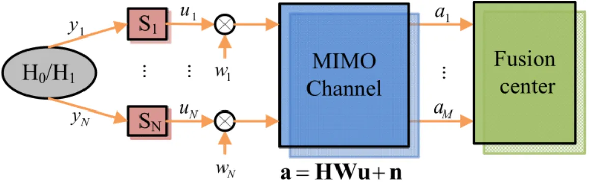
2.3 System model of MIMO channel . . . 11
3.1 Simple centralized detection . . . 14
3.2 N samples in the sensing time . . . 15
3.3 System model of optimal power allocation . . . 16
3.4 Two different distances . . . 21
3.5 System model of optimal power allocation . . . 23
3.6 Signal processing and without signal processing . . . 28
3.7 J-divergence and the detection probability of optimal power allocation and equal power allocation . . . 29
3.8 Detection probability and J-divergence of four cases in optimal power allocation . . . 30
3.9 The error probability of four cases in optimal power allocation . . . 31
3.10 The error probability and the lower bound of four cases in optimal power allocation . . . 31
3.11 The L2 distance and detection probability of optimal linear combination and equal weighting combination . . . 32
3.12 The L2 distance and detection probability of four cases in optimal linear combination . . . 33
3.13 MDC and L2 distance with fixed false alarm probability by the use of the simple detection . . . 36
3.14 Comparison between optimal power allocation, L2 distance, and MDC by
the use of Neyman-Pearson detection . . . 36
3.15 Simulated optimal detection probability and distance based detection prob-ability in optimal power allocation . . . 37
3.16 Simulated optimal detection probability and distance based detection prob-ability in optimal linear combination . . . 37
4.1 Truncated gaussian . . . 40
4.2 System model of censoring scheme . . . 41
4.3 Approximation of truncated Gaussian . . . 44
4.4 Structure of GMM J-divergence . . . 46
4.5 L2 distance optimal diagram . . . 54
4.6 System model of censoring scheme of optimal linear combination . . . . 55
4.7 The GMM J-divergence and detection probability of optimal power allo-cation censoring scheme . . . 59
4.8 The GMM L2 distance and detection probability of optimal power allo-cation censoring scheme . . . 60
4.9 The L2 distance and detection probability of optimal linear combination censoring scheme . . . 61
4.10 Comparison between censoring and non-censoring in the optimal power allocation . . . 63
4.11 Comparison between censoring and non-censoring in the optimal linear combination . . . 63
4.12 Comparison between the power of censoring scheme and the power of non-censoring scheme . . . 64
List of Tables
Chapter 1
Introduction
Cognitive radio has been viewed as a promising technology in next generation wireless communication networks striving for a better utilization of the wireless spectrum. In many countries, most of frequency bands are assigned to different wireless services. But some frequency bands are under-utilized. In [1], it has been shown that 70% of the allocated spectrum in the U.S. are not efficiently utilized. If we allow secondary users (unlicensed users) to use the frequency band of primary users (licensed users) when the primary users are idle, the utilization of spectrum will be enhanced. In other words, the main purpose of the cognitive radio systems is to utilize the spectrum and limit the interference to primary users in a efficient and intelligent manner.
• Related work:
There are many papers in cognitive radio. The work in [2]-[5] discuss the basic concepts and limitations of the cognitive radios. In [6], the authors propose 3 local sensing methods, the matched filter detection, the energy detection, and the cyclo-stationary feature detection. The detection probability of matched filter detection is optimal. In local sensing, it’s hard to distinguish between the noise and the weak signal because of deep fading. To improve the spectrum detection performance, cooperative spectrum sensing has been proposed in [7]-[19].
– Centralized detection
without quantization. In [10] and [11], the authors propose a cooperation scheme among secondary users to mitigate possible deep fading or shadow-ing, and thereby improve the detection probability. The work in [12], discuss several optimization methods in a linear combination system, which combines signals from all the antennas in the fusion center, with orthogonal channel in centralized detection. The work discusses 3 systems, conservative system, aggressive system, and hostile system, and a detection performance measure, modified deflection coefficient(MDC). But in this paper, it only concerns the orthogonal channel and doesn’t have any power constraint on secondary users.
– Distributed detection
The distributed detection is that the secondary users transmit the observation with quantization. Because of bandwidth constraint, it is often desirable to quantize data before transmitting. Many papers in distributed detection use only 1 bit. In distributed detection, we can reduce the data rate between fu-sion center and secondary users. But the detection performance of distributed detection is worse than centralized detection. The work in [13], discuss the semidefinite programming in distributed system in linear combination. The authors in [19] and [18] use distance measures to solve the power allocation problem. The work in [19] considers the approximated J-divergence, instead of the likelihood function, as the performance matric in distributed sensor net-work with multiple input multiple output(MIMO) channels, for the reason that the log likelihood ratio(LLR) does not have a closed-form expression and thus an explicit decision rule does not exist. In [18], the authors propose using ap-proximated J-divergence to approximate the J-divergence of gaussian mixture model. To have better detection probability, the authors adopt the element dis-tance measure, instead of the approximated J-divergence, as the performance matric in [19]. The work in [14] discusses the trade-off between the sensing time and throughput. If sensing time is shorter, the transmitting time is longer and the throughput is higher. The authors propose a multi-slot spectrum sens-ing scheme to maximize the detection probability of local senssens-ing. The
multi-slot spectrum sensing approach divides the sensing time into M mini-multi-slots and uses those slots to maximize the detection probability. This work also discusses the centralized detection and distributed detection to maximize the detection probability in cooperative spectrum sensing.
– Distance measure
In [17], the L2 distance approach is applied in the problem of speech recogni-tion. In addition, the work [20] and [21] discuss about fundamental properties of the distance measures. In [20], the J-divergence and B-divergence can lead to, respectively, a lower bound and an upper bound of the Bayesian error prob-ability.
– Censoring scheme
The work [22]-[23] propose a censoring scheme in which secondary users only transmit informative observation to the fusion center. The censoring scheme can reduce the interference to primary users. In [22], it transmits LLR to fusion center. When LLR is greater than a threshold, the user will transmit this LLR to fusion center or keep silent. In this paper, it discusses that the detection performance of one threshold is equal to the performance of two thresholds. In [23], it proposes a simple censoring scheme. By censoring the observation, only the users with enough information will transmit their local bit decision (0 or 1) to the fusion center. The detection probability and false alarm probability of spectrum sensing are investigated for both perfect and imperfect reporting channel.
• Motivation:
In this thesis, we still focus on the spectrum sensing problems in cognitive radio systems. When primary users use frequency bands, secondary users should be able to detect the existence of primary users. When secondary users transmit data or re-ceive data, they can’t cause intolerable interference on the primary users, if accurate detection fails.
when transmitting. However, when secondary users send signals to the fusion cen-ter for spectrum sensing, they should also have power constraint. In this thesis, we focus on the power constraint when secondary users are in the sensing phase. Here we use target signal to interference plus noise ratio(SINR) as the performance con-straint. The SINR of the primary users should be greater than the target SINR. We are interested in finding the weighting factor that maximizes the probability of de-tection while restricting the interference on the primary user within a predetermined level. In summary, our objectives in this research are,
– Maximize the detection probability.
– Satisfy the SINR constraint of primary users.
• Contributions:
– We use a distance measure of the probability distribution as the metric, instead
of the likelihood measure, to find the detection rule at the fusion center.
– We find the optimal power allocation scheme among secondary users and
op-timal linear combination approach in the fusion center, both to maximize the detection probability.
– We propose a censoring scheme in secondary users when transmitting signals
to the fusion center, attempting to lower interference while achieving accept-able performance.
In the first part of the thesis, we consider two schemes, namely the optimal power allocation and the optimal linear combination, in centralized cooperative spectrum sensing. Optimal power allocation scheme is that we control the power of every secondary user and optimize the detection probability. Optimal linear combination is that we combine the signal of every antenna by different weighting to maximize the detection probability. In centralized detection, it’s not easy to have the closed-form expression of detection probability and false alarm probability. But we can approach the detection probability, as promised by the likelihood detection rule,
by the use of distance measures. Analytical results show if the distance is larger, the detection probability is higher. In the second part of the thesis, we propose a censoring scheme in which secondary users transmit only the informative data to the fusion center. In censoring scheme, we use J-divergence and L2 distance to maximize the detection probability. Analytical results show that the censoring scheme have better detection probability than non-censoring schemes.
• Organization of the Thesis:
The thesis is organized as follows. In chapter 2, we talk about the fundamental concept of spectrum sensing in cognitive radio networks. In chapter 3, we intro-duce two different distance measures, the J-divergence and the L2 distance, in the optimal power allocation and optimal linear combination schemes. And the simu-lation results show that the performance are better than equal power allocation and equal linear combination. In chapter 4, we use the censoring method in optimal power allocation and optimal linear combination. And we show the simulation of the censoring method. Finally, chapter 5 gives the conclusion.
Chapter 2
Spectrum Sensing and System Model
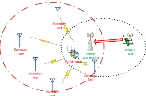
Cognitive Radio is the solution of the spectrum utilization. The users who have license are primary users. In some frequency bands, the spectrum utilization is not high. It means that primary users seldom use the frequency bands. Those frequency bands are under low utilization. To enhance the spectrum utilization, primary users should share their frequency bands to other users who don’t have the license. The users who want to use the frequency bands are secondary users. But one important thing is that secondary users should return the spectrum to primary users as soon as possible when primary users want to use and secondary users don’t cause much interference on primary users. Therefore, spectrum sensing is the key technique of cognitive radio. Secondary users should sense whether the primary users use the spectrum or not. If they are sure that primary users don’t use the spectrum now, they could use it. But there are still many problems in the spectrum sensing.
2.1
The Problems of Spectrum Sensing
The detection of the existence of primary user can be viewed as binary hypothesis. When
primary users exist, it’s under hypothesis H1. When primary users don’t exist and
sec-ondary users can use the spectrum, it’s under hypothesis H0.
The main problems we want to solve in spectrum sensing are:
• Minimize the false alarm probability Pf
• Minimize the sensing time
2.1.1
Detection Probability and False Alarm Probability
The definition of detection probability is
Pd= P ( ˆH = H1|H1). (2.1)
And the definition of false alarm probability is
Pf = P ( ˆH= H1|H0). (2.2)
ˆ
H means secondary users make a decision which hypothesis is possible. Pd means the
probability that the secondary users decide H1 hypothesis and primary users is really
using the spectrum. Pf means the probability the secondary users decide H0 hypothesis
and primary users is not really using the spectrum. Obviously, the system performance
will be better if Pdis higher and Pf is lower. When Pdis higher, secondary users won’t
use the spectrum when primary users exist. When Pf is lower, it means the spectrum
utilization is higher.
ŔŦůŴŪůŨġŵŪŮŦ
ŕųŢůŴŮŪŵŵŪůŨġŵŪŮŦ
2.1.2
Sensing Time
Because we can’t exactly know when primary users want to use the spectrum, we peri-odically sense the spectrum to solve this problem. Fig. 2.1 shows that it can be separated into the sensing time and the transmitting time. It is obvious that the sensing time should be short. In other words, if the sensing time is too long, the transmitting time will be short and the average data rate will be low. But in our system model, we assume a fixed sensing time and periodically sense the spectrum.
2.2
Maximize the Detection Probability
Why should we maximize the detection probability? The reason is that secondary users should return the spectrum when the primary users exist. The definition of detection probability is that we decide primary users is using the spectrum and primary users is really using the spectrum. Therefore, when secondary users detect the primary users is using the spectrum, secondary users will stop transmitting data. When the detection probability is low, secondary users will frequently use the spectrum to transmit data when primary users exists, like in Fig. 2.2. It may cause intolerance interference on primary users.
2.2.1
Local Sensing
Local sensing means every secondary user makes his own decision without cooperation. In [6], there are 3 methods to implement the local detection. For example, matched fil-ter detection. The matched filfil-ter detection maximizes the signal-to-noise ratio. But the matched filter detection needs to know the prior knowledge of primary users signal at both PHI and MAC layers. It’s not practical. Energy detection is another method. It collects the energy of every sensing sample. But the energy detection still has drawbacks. For ex-ample, how to decide the threshold of the decision rule. Obviously, the local sensing will depends on the power of primary users, the channel between primary users and secondary users, and so on. For example, if the signal of primary users is weak, the detection
proba-Figure 2.2: Interference of primary users
bility of secondary users will be low and the secondary users will transmit data frequently. To avoid this problem, we should consider cooperative spectrum sensing to enhance the detection probability.
2.2.2
Cooperative Sensing
Cooperative sensing means some secondary users cooperate with each other to enhance the detection probability. Many papers use cooperative scheme because of poor perfor-mance of local sensing. In the cooperative spectrum sensing, every secondary user sends the data to the fusion center. The fusion center can be viewed as a common receiver of secondary users. Because the fusion center has more data than every secondary user, it can have more accuracy detection. There are two schemes to solve the cooperative spec-trum sensing, centralized detection and distributed detection. The centralized detection is that every secondary user transmits unquantized observation to the fusion center. Then the fusion center uses the observations to make the decision. The distributed detection is that every secondary user transmits quantized signal to the fusion center, like ”-1” and
”1”. ”-1” means H0 hypothesis and ”1” means H1hypothesis. In [14], it uses the
of ”1” at the fusion center, the fusion center will decide H0 hypothesis. Obviously, the
performance of the centralized detection is better than the distributed detection. And in [10], secondary users can sense lower power of primary users than local sensing because of cooperation. We can enhance the performance by the use of the cooperative spectrum sensing. The following section will discuss our system model of the cooperative spectrum sensing.
2.3
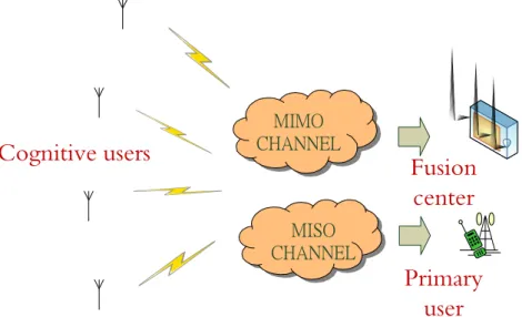
System Model
Fig. 2.3 shows the system model. Firstly, secondary users sense data for detecting the ex-istence of the primary user. Here we use multiple input multiple output (MIMO) channel between secondary users and the fusion center. Every user sends the data to the fusion center for the cooperative spectrum sensing and the fusion center has multiple antennas. Every secondary user has only one antenna. It is reasonable because secondary users of-ten have the power constraint. There is only one primary user and the primary users has only one antenna. Assume every secondary user uses the same spectrum in sensing time and in transmitting time. Obviously, it will produce a problem. When secondary users transmit their sensing data to the fusion center for spectrum sensing and primary users want to access spectrum in the same time, the data of secondary users transmitting may cause intolerance interference to the primary user. This problem should be avoided. We list the problems we should solve:
• Maximize the detection probability • Minimize the false alarm probability
• Minimize the interference when cooperative spectrum sensing • Minimize sensing time
But in our system model, the sensing time will be a fixed time for simplicity. The detection probability and the interference of primary users should be minimized. Assume the power of the primary user is known by the fusion center. When secondary users
Primary
user
Cognitive users
Fusion
center
ŎŊŎŐ ńʼnłŏŏņō ŎŊŔŐ ńʼnłŏŏņōFigure 2.3: System model of MIMO channel
transmit the data to the fusion center and the primary user exists, we can set a target
SINR, SIN Rt, for the primary user and the SINR of the primary user should be greater
than SIN Rt.
The equation of SINR is
SIN Rp =
PP
PN
i hpiPsi + σn2
, (2.3)
where Psi is the transmitting power of ith secondary user, hpi is the channel between
secondary users and the primary user, N is the number of secondary users, and σn2 is the
variance of noise.
Therefore, the capacity of the primary user is
CP =
1
2log(1 + SINRp) ≥
1
2log(1 + SINRt), (2.4)
where Cp is the capacity of the primary user.
If the SIN Rt is high, it means that the primary user can’t allow much interference
from secondary users and the secondary users can’t use much power for transmission. In other words, we should satisfy the quality of service (QoS) requirement of the primary user. Therefore, it should have power constraint on secondary users. And the final objec-tive is to optimize the detection probability under the SINR constraint. In the following
chapters, we will discuss how to satisfy the target SINR and optimize the detection prob-ability.
Chapter 3
Centralized Detection in Optimal Power
Allocation and Optimal Linear
Combination
3.1
Introduction
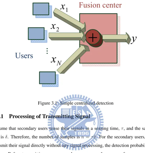
In cooperative spectrum sensing, every secondary user transmits the observation to the fusion center. The fusion center can use those observations to have accuracy detection. If all secondary users send their data to the fusion center without quantization, this is called centralized detection. For example, consider a simple centralized detection scheme. Fig. 3.1 shows the system model. Every secondary user transmits the observation to the fusion center. From Fig. 3.1, the received signal of the fusion center is
y=
N
X
i=1
xi, (3.1)
where xiis the signal from the ith secondary user and there are N secondary users.
Then the fusion center uses this signal, y, to make the decision. A simple decision method is that whether the value of y is greater than γ or not. If y is greater than γ, we
can decide that it is under hypothesis H1.
In this thesis, we consider two optimization schemes, optimal power allocation and optimal linear combination.
įįį
1
x
2
x
N
x
y
Figure 3.1: Simple centralized detection
3.1.1
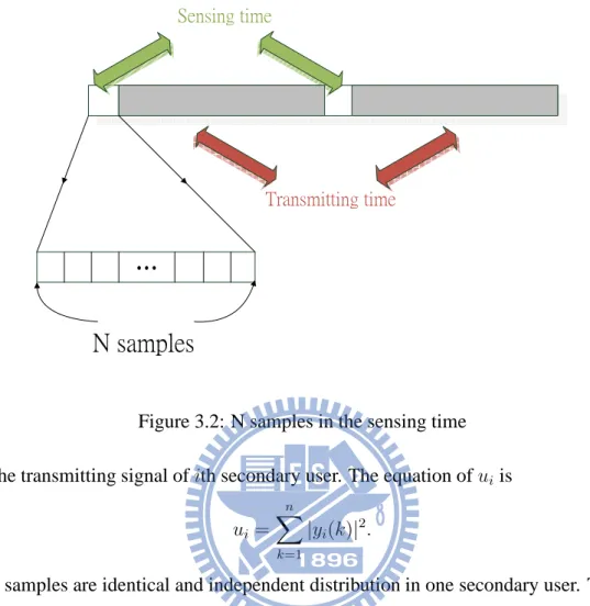
Processing of Transmitting Signal
Assume that secondary users sense their signals in a sensing time, τ , and the sampling
rate is δ. Therefore, the number of samples is n = τ δ. For the secondary users, if they
transmit their signal directly without any signal processing, the detection probability will be low. Before transmitting, every secondary user sums the square of every sample and transmits it to the fusion center. The equation of the sensing signal of ith secondary user in kth sample is yi(k) = vi(k), under H0 hpis(k) + vi(k), under H1, (3.2)
where yi(k) is the signal sensed by ith secondary user, vi(k) is the sensing noise and its
distribution is N(0, σ2
vi), s(k) is the signal of the primary user, k means kth sample, and
hpiis the channel between ith secondary user and the primary user. Assume all sensing
samples in one secondary user are independent. The overall power of primary user in n samples is
Es=
n
X
k=1
ŔŦůŴŪůŨġŵŪŮŦ
ŕųŢůŴŮŪŵŵŪůŨġŵŪŮŦ
įįį
ŏġŴŢŮűŭŦŴ
Figure 3.2: N samples in the sensing time
uiis the transmitting signal of ith secondary user. The equation of ui is
ui = n
X
k=1
|yi(k)|2. (3.4)
The n samples are identical and independent distribution in one secondary user. The
dis-tribution of uican be viewed as a non-centralized Chi-square distribution with n degrees.
If n is large enough, it can be asymptotical to a Gaussian distribution by the central limit theorem.
After some computation, the asymptotical distribution of ui is:
E[ui] = nσv2i, under H0 (n + ηi)σv2i, under H1 (3.5) and V ar[ui] = 2nσ4 vi, under H0 2(n + 2ηi)σv4i, under H1, (3.6) where ηi = |hpi| 2E s σ2
vi . Therefore, the distribution can be represented as a Gaussian random
variable.
In the simulation result, it will prove the detection probability will be higher after the signal processing.
3.2
Optimal Power Allocation
In optimal power allocation scheme, we multiply weighting factor to the transmitting signal of every secondary user. There are two reasons why we multiply weighting factor to transmitting signal.
• Maximize the detection probability • Satisfy the power constraint
In the following sections, we will discuss the optimal power allocation.
3.2.1
System Model
In the cognitive radio environment, assume that there are N secondary users and the fusion center has M receiving antennas. To simplify the system, there is only one primary user. The primary user and every secondary user only has one antenna.
Our objective is to maximum the global detection probability, PD, and reduce the
interference to primary users when secondary users transmit data to the fusion center. In other words, when the primary users use the frequency bands, the secondary users can’t produce the intolerance interference to primary users. The Fig. 3.3 shows the system model. In the centralized method, secondary users send their observation to the fusion center for the detection. But we should guarantee the QoS requirement of primary users.
1 N
įįį
įįį
0 1įįį
n
HWu
a
!
1u
Nu
1y
Ny
ʹ 1w
Nw
ʹ 1a
Ma
In other words, we should guarantee the SINR of the primary users should be greater than
one determined value, SIN Rt. The secondary users can not transmit their signal directly
because of the power constraint. They should have the weighting factors for the power control.
The received signal of the fusion center is
a= HWu + n, (3.7) where a= a1 a2 .. . aM , H= h11 h12 ... h1N h21 h22 ... h2N .. . ... . .. ... hM1 hM2 ... hM N , W= w1 0 ... 0 0 w2 ... 0 .. . ... . .. 0 0 0 ... wN , u= u1 u2 .. . uN , n = n1 n2 .. . nM
u is the signal vector transmitted by secondary users, W= diag([w1, w2, ..., wN]T) is the
power control, H is channel matrix between the fusion center and the secondary users, n ∼ N(0, σn2IM×M) is the noise received by the fusion center, and a is the signal received
of the fusion center.
Assume that the signals sensed by the secondary users are independent. Therefore, we can have the distribution of u.
p(u|Hi) = 1 |2πσ2 ui| 1 2 exp[−12(u − Ei)Tσ2ui −1 (u − Ei)], (3.8) where σu21 = 2(n + 2η1)σv4 0 ... 0 0 2(n + 2η2)σ4v ... 0 .. . ... . .. 0 0 0 ... 2(n + 2ηN)σ4v
, σu20 = 2nσ4 v 0 ... 0 0 2nσ4 v ... 0 .. . ... . .. 0 0 0 ... 2nσ4 v , E1 = (n + η1)σ2v (n + η2)σ2v .. . (n + ηN)σv2 , E0 = nσ2 v nσv2 .. . nσv2
From the equation (3.8), we can have the distribution of a. p(a|Hi) = 1 |2πΣi| 1 2 exp[− 1 2(a − µi) TΣ−1 i (a − µi)], (3.9) where Σi = HWσ2uiW T HT + σn2I (3.10) and µi = HWEi. (3.11)
Then we can discuss the detection method by the use of the likelihood ratio test.
3.2.2
The Performance Matric of Detection Probability
The final goal of our scheme is to maximum the detection probability. In the Neyman-Pearson detection, we should calculate likelihood ratio firstly. By the use of the likelihood ratio, we can have the detection probability.
L(a) = p(a|H1) p(a|H0) = 1 |2πΣ1| 1 2 exp[− 1 2(a − µ1) TΣ−1 1 (a − µ1)] 1 |2πΣ0| 1 2 exp[− 1 2(a − µ0)TΣ−10 (a − µ0)] H1 ≷ H0 γ, (3.12)
Therefore, the log likelihood ratio (LLR) is l(a) = ln|Σ0| 1 2 |Σ1| 1 2 + (− 1 2(a − µ1) TΣ−1 1 (a − µ1)) −(−1 2(a − µ0) TΣ−1 0 (a − µ0)) ≷HH10ln γ.
From equation (3.10) and equation (3.11), the log likelihood ratio is l(a) = ln|Σ0| 1 2 |Σ1| 1 2 + (− 1 2(a − µ1) TΣ−1 1 (a − µ1)) − (−12(a − µ0)TΣ−10 (a − µ0)) = ln|Σ0| 1 2 |Σ1| 1 2 + 1 2a T(Σ−1 0 − Σ−11 )a + aT(Σ−11 µ1− Σ−10 µ0) + 12µT1Σ−10 µ1−21µT0Σ−10 µ0 = ln|HWσ2u0WTHT+σ2nI| 1 2 |HWσu21WTHT+σn2I| 1 2 +12aT((HWσ2 u0WTHT + σn2I)−1− (HWσ2u1WTHT + σ2nI)−1)a +aT((HWσ2 u1WTHT + σn2I)−1(HWE1) − (HWσu20WTHT + σn2I)−1(HWE0)) +12(HWE1)T(HWσ2u1WTHT + σn2I)−1(HWE1) −1 2(HWE0) T(HWσ2 u0WTHT + σn2I)−1(HWE0). (3.13)
Therefore, the detection probability, PD, is
PD = P (l(a) > ln γ|H1). (3.14)
The optimization problem is
maxW PD
s.t. Psi ≤ Pc
SIN Rp ≥ SINRt.
(3.15)
Psiis the power of ith secondary user and Pc is the power constraint of secondary users.
The equation of SIN Rp is
SIN Rp = Pp P ih2piw 2 iPsi+ σ2np , (3.16)
where Pp is the power of the primary user, hpi is the channel between the primary user
and ith secondary user, and σn2pis the noise power of the primary users.
Because l(a) is a nonlinear combination of a, it is difficult to calculate the distribution
of l(a). Obviously, it’s hard to have the closed-from expression of the detection
Therefore, it’s hard to use the likelihood ratio based detection for optimization. But we can use the performance matric, such as the distance measure, instead of calculating the detection probability directly. We use this performance matric to optimize the detection probability. In the following sections, we will introduce the distance based detection by the use of J-divergence in the optimal linear combination.
J-divergence
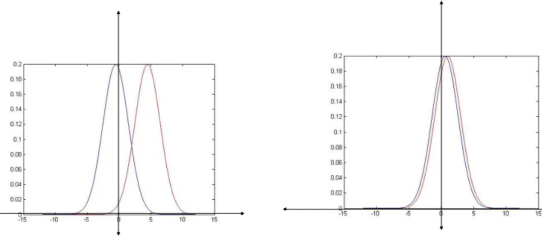
J-divergence is a distance measure. For example, if we have two random variables, the distance measure can be viewed as the distance between this two random variables. If the distance between them is long, we can easily distinguish them and the detection proba-bility will be high. Like in the Fig. 3.4, if distance between them is small, it’s not easy to justify which hypothesis really exists. Under this condition, it’s easy to make a fault deci-sion. In the distance measure method, the objective is to maximize the distance between two distributions.
The error probability is defined as
Pe= P (H0)P (l(a) > ln γ|H0) + P (H1)P (l(a) < ln γ|H1) (3.17)
, and J-divergence can provide the lower bound of Pe[20].
Pe> P(H0)P (H1)e(−
J
2), (3.18)
where P(H0) is the probability that primary users don’t use the spectrum and P (H1) is
the probability that primary users use the spectrum.
From the above equation, we can use the J-divergence for replacing calculate the error probability directly. The definition of J-divergence is
J = E1[(L − 1) ln L] =R+∞ −∞[(L − 1) ln L]p1(x)dx (3.19) where L(x) = p0(x) p1(x).
In our case, L(x) = P(a|H0)
P(a|H1). J-divergence is the symmetric form of the
Kullback-Leibler (KL) distance.
(a) Long distance (b) Small distance
Figure 3.4: Two different distances
where DKL(.) is the KL distance. The definition of the KL distance is
DKL(F ||G) = −P f (x) log g(x) + P f (x) log f (x)
= H(F, G) + H(F ),
(3.21)
where H(F, G) is the cross entropy and H(F ) is the entropy of F . The physical mean of
the KL distance is expected number of extra bits using a code based on G rather than F . If the distance is larger, it will use more bits to transmit.
By adopting J-divergence as the performance matric, the optimization problem be-comes to
maxW J(p(a|H0), p(a|H1))
s.t. Psi ≤ Pc
SIN Rp ≥ SINRt.
(3.22)
After computation, we can using the variance and mean of a to calculate the value of J-divergence,
J(p(a|H0), p(a|H1)) = 1
2Tr[Σ0Σ−11 + Σ1Σ−10 + (Σ−10 + Σ−11 )(µ1− µ0)(µ1− µ0)T] − M.
(3.23)
Therefore, we can use the optimization method to find the maximum value of J-divergence in the optimal power allocation.
Here we discuss a special condition. Assume the received SNR of the fusion center is
low. Let E= (E1−E0) and HWσu2iWTHT ≪ σn2I. Therefore, Σi ≃ σn2I. The equation
(3.23) becomes to J(p(a|H0), p(a|H1)) = 12Tr[σn2I σ2 nI + σ2nI σ2 nI + (2(σ 2 nI)−1(HWE)(HWE)T)] − M = σ12 nTr(HWEE TWTHT) = σ12 nTr(E TWTHTHWE) = σ12 nE TWTHTHWE. (3.24)
Let w= [w1, w2, ..., wN]T. The equation (3.24) becomes to
J(p(a|H0), p(a|H1))
= 1
σ2 nw
Tdiag(E)HTHdiag(E)w. (3.25)
Obviously, the equation (3.25) is a convex function. Therefore, when the receiving SNR of the fusion center is low, J-divergence is a convex function. Here we can’t prove the J-divergence only has the global optimal solution. We may only find the local maximum by the optimization method. We only know that J-divergence will be a convex function under low SNR condition. But in simulation, the optimal power allocation by the use of J-divergence has much better detection probability than the equal power allocation.
3.3
Optimal Linear Combination
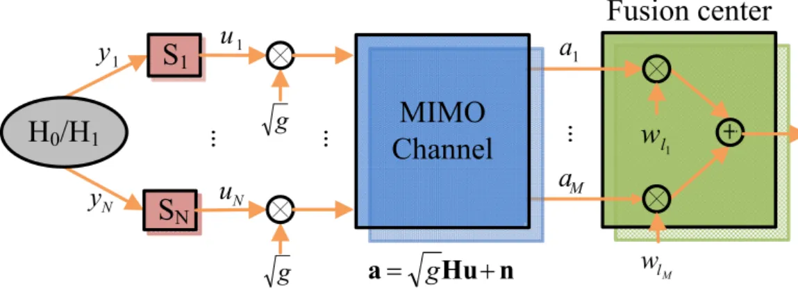
In the optimal linear combination, we combine the received signal by every antenna with weighting factors, like in the Fig. 3.5. Therefore, the signal which we want to detect becomes to
a=√gHu+ n, (3.26)
where a = [a1, a2, ..., aM]T, H = [˜h1, ˜h2, ..., ˜hM], and ˜hi is N × 1 channel vector,
i = 1, 2, ..., M. √g is the power control and it is a constant. The power summation
of all secondary users can not exceed Pc. For simplicity, let the power summation of all
secondary users are equal to Pc. Then the value of g is
g
N
X
i=1
įįį
įįį
įįį
ʹ ʹn
Hu
a
! g
1 lw
M lw
1y
Ny
1a
Ma
1 N 0 1 1u
ʹ g Nu
ʹ gFigure 3.5: System model of optimal power allocation
From the above equation, we can calculate g. The value of Pc is decided by SIN Rt. In
other words, g = w1 = w2 = ... = wN in the optimal linear combination.
aiis the received signal by the ith antenna. It is the Gaussian distribution and its mean
and variance are
Eai|Hj = √g˜hT i Ej (3.28) and V arai|Hj = g˜h T i σ 2 uj˜hi+ σ2. (3.29)
The fusion center can detect the primary users by the signal, r.
r = M X i wliai = w T l a, (3.30) where wl = [wl1wl2...wlM]
T. r is a Gaussian random variable and its mean and variance
are Er = √gw lTHE0, under H0 √gw lTHE1, under H1 (3.31) and V arr = wT l (gHσ 2 u0HT + σn2I)wl, under H0 wlT(gHσ2u1HT + σn2I)wl, under H1. (3.32) Here we use another distance measure, L2 distance, in the optimal linear combination. J-divergence can’t optimize in the optimal linear combination. The definition of L2 distance
is
DL2 =
Z
(f1 − f2)2dx, (3.33)
where f1and f2 are two distribution functions.
Here we use the aiin L2 distance instead of r. The L2 distance scheme can be viewed
as that the fusion center linearly combines the distribution of every antenna. Obviously, the distribution of r is not the linear combination of the distribution of every antenna. But in the simulation result, L2 distance will have better detection probability than other distance measure.
Rewrite the equation (3.33) as Z
(wT
l PaH1 − wTl PaH0)2dx, (3.34)
where wl = [wl1, wl2, ..., wlM]
T and P
aHi = [p(a1|Hi), p(a2|Hi), ..., p(aM|Hi)]T.
From equation (3.28) and (3.29), ai is a Gaussian random variable. The L2 distance
can be write as DL2(wTl PaH1, wTl PaH0) =R (wTl PaH1 − wTl PaH0)2dx =R [(wT l Pa H1) 2− 2wT l Pa H1w T l Pa H0 + (w T l Pa H0) 2]dx =P i P jwliwljR p(ai|H1)p(aj|H1)dx −2P i P jwliwljR p(ai|H1)p(aj|H0)dx +P i P jwliwljR p(ai|H0)p(aj|H0)dx. (3.35)
Assume two Gaussian random variables have the means, µaand µb, and the variances,
σ2aand σb2. The integration of this two random variables is
Z N(x, µa, σa2)N(x, µb, σ2b)dx = 1 pdet(2π(σ2 a+ σb2)) e−12(µa−µb)T(σa2+σ2b)−1(µa−µb). (3.36) Therefore, we can rewrite all the multiplications of two Gaussian random variables by the
use of three matrices, M11, M10, and M00.
M11ij = Z p(ai|H1)p(aj|H1)dx. (3.37) M10ij = Z p(ai|H1)p(aj|H0)dx. (3.38)
M00ij = Z
p(ai|H0)p(aj|H0)dx. (3.39)
The equation of L2 distance which we want to optimize is DL2(wTl PaH1, wTl PaH0) =PiPjwliwljM 11 ij − 2 P i P jwliwljM 10 ij +P i P jwliwljM 00 ij = wT l M11wl− 2wTl M10wl+ wlTM00wl = wT l (M11− 2M10+ M00)wl. (3.40)
Obviously, the equation we want to optimize is a convex problem. If we don’t have
any constraint on wl, the value of the L2 distance will become to infinity. To avoid this
problem, let wlTwl = 1. Therefore, the optimization problem becomes to
maxwl DL2(wlTPaH1, wlTPaH0) = wlT(M11− 2M10+ M00)wl
s.t. wli ≥ 0, i = 1, 2, ..., M
wT
l wl= 1.
(3.41)
The optimization problem can be easily solved by the optimization method. Here we use the active set method. The active set method is that checking the inequality constraints are active or not. If the inequality constraints are active, we can view the inequality con-straints as the equality concon-straints and use the Lagrange multiplier to solve this problem. If all the computation results satisfy the Karush-Kuhn-Tucker (KKT) condition, it’s one iteration. After several iterations, we can find the optimal solution.
Then we discuss a simple decision rule:
r > t, (3.42)
where t is the detection threshold. The equation (3.31) and (3.32) show the distribution of r. It’s easy to calculate the detection probability and the false alarm probability. The equations of the detection probability and the false alarm probability are
PD = Q( t− Er|H1 pV arr|H1 ) (3.43) and Pf = Q( t− Er|H0 pV arr|H0 ). (3.44)
The optimal linear combination is simpler than the optimal power allocation. The optimal linear combination uses g for the power control. Every secondary user uses the same scalar, g. Therefore, the fusion center can broadcast g to secondary users. But the optimal power allocation should tell secondary users their own weighting factors. In the L2 distance method, the antenna which has the better L2 distance, its weighting will be larger. For example, if there are 2 antennas, the L2 distance of the first antenna is greater than the second antenna, its weighting is larger.
3.4
Simulation Results
In this section, we present the simulation by the use of the distance measures. Assume the MIMO channel and the noise are all random and the power of the primary user is known. The SNR of the primary user is 5. The probability that primary users use the frequency band is 0.2 and the probability that don’t use the frequency band is 0.8 because the primary users seldom exist. In the following, we will discuss simulation of the optimal power allocation and the optimal linear combination.
3.4.1
Optimal Power Allocation
In the optimal power allocation scheme, the distance measure is J-divergence . In this scheme, the decision rule is Neyman-Pearson detection at the fusion center. We set that the false alarm probability is 0.4. It means that the spectrum utilization is 60% in this simulation environment. As we mentioned before, it’s hard to calculate and optimize the detection probability directly because LLR is not a linear combination of a. Therefore, we simulate the detection probability by the Monte Carlo method.
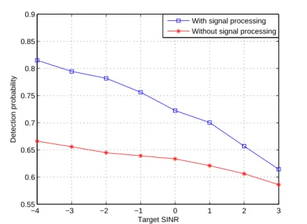
Fig. 3.6 shows two different transmitting signals of secondary users. If the signal doesn’t have any signal processing and transmits it directly to the fusion center, its detec-tion probability is worse than the signal with the signal processing. Obviously, it’s trade off between the sensing time and the detection probability because the signal with the signal processing needs more sensing samples.
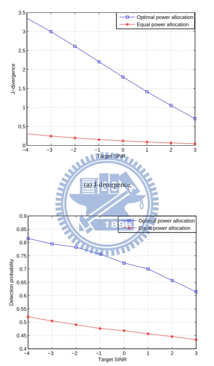
the target SINR is high, it means that the total power of secondary users can use is low. In the equal power allocation, the detection probability of J-divergence is lower than the optimal power allocation. But only Fig. 3.7(a) can’t prove the J-divergence can be viewed as a performance matric.
Fig. 3.7(b) shows the detection probability. In Fig. 3.7(a) and Fig. 3.7(b), we can observe that when the value of J-divergence is higher, the detection probability is higher. Therefore, J-divergence can be a performance matric in the optimal power allocation. And in Fig. 3.7(b), the detection probability of the optimal power allocation is much better than equal power allocation.
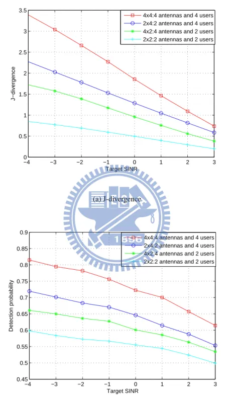
Fig. 3.8(a) shows four cases, 2x2, 2x4, 4x2, and 4x4. 4x2 means there are 4 receive antennas and 2 secondary users in the simulation, and so on. Obviously, the more antennas or the more secondary users, the better performance. Therefore, the fusion center can have benefit by using the MIMO channel in the optimal linear combination. Then compare the 2x4 case and the 4x2 case. In this figure, the 2x4 case is better than the 4x2 case. The reason is that it optimizes the detection probability by multiplying the weighting factors to secondary users in the optimal power allocation. If there are more users, we can have more degrees of freedom. Therefore, if there are more users or more receiving antennas of the fusion center in cognitive radio system, the detection probability will be better. But increasing the number of secondary users is better than increasing the number of receiving antenna of the fusion center. Fig. 3.9 shows the error probability and the lower bound. If the target SINR is lower, the error probability will also be lower. From the equation
(3.18), Pe> P(H0)P (H1)e(−
J
2), the error probability has a lower bound. Fig. 3.10 shows
this property.
3.4.2
Optimal Linear Combination
In this simulation, we also use the Neyman-Pearson decision rule in the fusion center. And in the later section, we will compare the performance between the optimal power allocation and the optimal linear combination.
Fig. 3.11(a) shows the simulation result of the optimal linear combination by using L2 distance. In this figure, when target SINR is high, it means the power that secondary
−4 −3 −2 −1 0 1 2 3 0.55 0.6 0.65 0.7 0.75 0.8 0.85 0.9 Target SINR Detection probability
With signal processing Without signal processing
Figure 3.6: Signal processing and without signal processing users can use for transmitting is low and the L2 distance is small.
Fig. 3.11(b) shows the detection probability. This figure can tell us that L2 distance can be really as a performance matric. When the L2 distance is larger, the detection prob-ability is larger. Therefore, we can use this distance measure to maximize the detection probability in the linear combination.
Fig. 3.12(a) shows the four cases of optimal linear combination, 2x2, 2x4, 4x2, 4x4. In this figure, the 4x2 case is better than the 2x4 case. The reason is that it optimizes the detection probability by the use of the weighting factor of every receive antenna in the optimal linear combination. Therefore, if there are more antennas in the fusion center, the degree of freedom is high. Increasing the number of receiving antennas of the fusion center is better than increasing the number of secondary users. Fig. 3.12(b) shows the detection probability. In this figure, when L2 distance is high, the detection probability will also be high.
3.4.3
Comparison
In this subsection, we will compare 2 schemes, the optimal power allocation and the optimal linear combination.
−4 −3 −2 −1 0 1 2 3 0 0.5 1 1.5 2 2.5 3 3.5 Target SINR J−divergence
Optimal power allocation Equal power allocation
(a) J-divergence −4 −3 −2 −1 0 1 2 3 0.4 0.45 0.5 0.55 0.6 0.65 0.7 0.75 0.8 0.85 0.9 Target SINR Detection probability
Optimal power allocation Equal power allocation
(b) Detection probability
Figure 3.7: J-divergence and the detection probability of optimal power allocation and equal power allocation
−4 −3 −2 −1 0 1 2 3 0 0.5 1 1.5 2 2.5 3 3.5 Target SINR J−divergence
4x4:4 antennas and 4 users 2x4:2 antennas and 4 users 4x2:4 antennas and 2 users 2x2:2 antennas and 2 users
(a) J-divergence −4 −3 −2 −1 0 1 2 3 0.45 0.5 0.55 0.6 0.65 0.7 0.75 0.8 0.85 0.9 Target SINR Detection probability
4x4:4 antennas and 4 users 2x4:2 antennas and 4 users 4x2:4 antennas and 2 users 2x2:2 antennas and 2 users
(b) Detection probability
Figure 3.8: Detection probability and J-divergence of four cases in optimal power alloca-tion
−4 −3 −2 −1 0 1 2 3 0.35 0.36 0.37 0.38 0.39 0.4 0.41 0.42 0.43 0.44 Target SINR Error probability
4x4:4 antennas and 4 users 2x4:2 antennas and 4 users 4x2:4 antennas and 2 users 2x2:2 antennas and 2 users
Figure 3.9: The error probability of four cases in optimal power allocation
−4 −3 −2 −1 0 1 2 3 0 0.1 0.2 0.3 0.4 0.5 0.6 0.7 Target SINR Error probability
4x4:4 antennas and 4 users, error probability 2x4:2 antennas and 4 users, error probability 4x2:4 antennas and 2 users, error probability 2x2:2 antennas and 2 users, error probability 4x4:4 antennas and 4 users, lower bound 2x4:2 antennas and 4 users, lower bound 4x2:4 antennas and 2 users, lower bound 2x2:2 antennas and 2 users, lower bound
Figure 3.10: The error probability and the lower bound of four cases in optimal power allocation
−4 −3 −2 −1 0 1 2 3 0.44 0.46 0.48 0.5 0.52 0.54 0.56 0.58 0.6 0.62 Target SINR Detection probability
Optimal linear combination Equal weight combination
(a) L2 distance −4 −3 −2 −1 0 1 2 3 0.02 0.04 0.06 0.08 0.1 0.12 0.14 0.16 0.18 Target SINR L2 distance
Optimal linear combination Equal weight combination
(b) Detection probability
Figure 3.11: The L2 distance and detection probability of optimal linear combination and equal weighting combination
−4 −3 −2 −1 0 1 2 3 0.02 0.04 0.06 0.08 0.1 0.12 0.14 0.16 0.18 Target SINR L2 distance
4x4:4 antennas and 4 users 4x2:4 antennas and 2 users 2x4:2 antennas and 4 users 2x2:2 antennas and 2 users
(a) L2 distance −4 −3 −2 −1 0 1 2 3 0.48 0.5 0.52 0.54 0.56 0.58 0.6 0.62 Target SINR Detection probability
4x4:4 antennas and 4 users 4x2:4 antennas and 2 users 2x4:2 antennas and 4 users 2x2:2 antennas and 2 users
(b) Detection probability
Figure 3.12: The L2 distance and detection probability of four cases in optimal linear combination
By the equation (3.43) and (3.44), we can calculate PD and Pf by the use of a simple
detection method in the optimal linear combination. In [12], it focuses on the optimization of optimal linear combination in the cognitive radio and proposes 3 optimization methods in 3 different systems, conservative system, aggressive system, and hostile system. In this paper, we can know the optimization of the equation (3.43) is hard. Only in the aggressive system, the equation (3.43) is a convex problem. But in the final part of this paper, it proposes a modified deflection coefficient (MDC) method. In the MDC method, it’s also a distance measure and combines the receiving data of every antenna in the fusion center. In other words, it’s also a distance measure in the optimal linear combination. Let h′ = [h2
11h222...h2N N]T.
The definition of the MDC is
d2m(wl) =
(Esh′Twl)2
wT
l V arrwl
. (3.45)
And the optimization problem is
maxwl d2m(wl)
s.t. wTl wl = 1.
(3.46)
and let w′l = V ar−T2
r|H1h
′. The optimal solution of equation (3.46) is
wlopt = V ar− 1 2 r|H1w ′ l kV ar−12 r|H1w ′ lk2 . (3.47)
Fig. 3.13 shows the comparison between the MDC method and the L2 distance method.
Consider a simple decision rule, r > t. In this decision rule, we can fix the value of Pf
and maximize the detection probability. In Fig. 3.13, the detection probability of the L2 distance method is little better than the detection probability of the MDC method under the same false alarm probability. But in [12], the system model of the MDC method is in the orthogonal channel. But L2 distance can also use not only in the orthogonal channel. The L2 distance method is more general than the MDC method.
Fig. 3.14 shows the detection probability of 3 schemes, optimal power allocation, optimal linear combination, and MDC. This simulation uses 2 secondary users and 2 receiving antennas in the fusion center. In this simulation, the decision criterion in the
fusion center is the Neyman-Pearson detection. The performance of the optimal linear combination is the best and the MDC is the worst. The optimal power allocation is the best because it controls the power of secondary users. If one of secondary users has lower sensing noise or receives a stronger signal from primary users, it will have more transmitting power and the fusion center can be more sure which hypothesis is right. The optimal linear combination only combines the received data, so it can’t have benefit on the data directly. Therefore, the detection probability of the optimal linear combination is worse than the detection probability of the optimal power allocation.
The MDC method also uses in the optimal linear combination, like L2 distance. But comparing to L2 distance, the MDC method only uses variance and mean for the maxi-mization, it’s worse than the L2 distance method in the simulation results.
Fig. 3.15 and Fig. 3.16 show that the simulated optimal detection probability and the distance based detection probability. In this figure, we can know the distance based detection probability will smaller than the real optimal detection probability. But the com-putation complexity of the distance based detection method is much lower than finding the optimal detection probability exhaustedly.
0.1 0.2 0.3 0.4 0.5 0.6 0.7 0.8 0.9 0.2 0.3 0.4 0.5 0.6 0.7 0.8 0.9 1
prob. false alarm
detection probability
optimal linear combination 6x6 L2 distance
MDC
Figure 3.13: MDC and L2 distance with fixed false alarm probability by the use of the simple detection −4 −3 −2 −1 0 1 2 3 0.4 0.45 0.5 0.55 0.6 0.65 0.7 0.75 0.8 0.85 0.9 Target SINR Detection probability
Optimal power allocation L2 distance
MDC
Figure 3.14: Comparison between optimal power allocation, L2 distance, and MDC by the use of Neyman-Pearson detection
−4 −3 −2 −1 0 1 2 3 0.48 0.5 0.52 0.54 0.56 0.58 0.6 0.62 0.64 0.66 Target SINR Detection probability Simulated optimal Distance based
Figure 3.15: Simulated optimal detection probability and distance based detection proba-bility in optimal power allocation
−4 −3 −2 −1 0 1 2 3 0.48 0.5 0.52 0.54 0.56 0.58 0.6 0.62 0.64 0.66 0.68 Target SINR Detection probability Simulated optimal Distance based
Figure 3.16: Simulated optimal detection probability and distance based detection proba-bility in optimal linear combination
3.5
Summary
In this chapter, we discuss the optimal power allocation and the optimal linear combi-nation. We adopt J-divergence as a performance matric in the optimal power allocation and adopt L2 distance as a performance matric in the optimal linear combination. In the optimal power allocation, the detection probability is better than the detection probability in the equal power allocation. The detection probability of the optimal linear combi-nation is better than the detection probability of the equal weighting combicombi-nation, too. If two schemes use the same decision rule, such as the Neyman-Pearson detection rule, the detection probability of the optimal linear combination is worse than the detection probability of the optimal power allocation. But as mentioned before, the optimal linear combination is simpler than the optimal power allocation.
Chapter 4
Censoring Scheme in Centralized
Detection
4.1
Introduction
In the cognitive environment, when secondary users transmit their observations to the fusion center, they should reduce interference when primary users exists. Here we propose a new method, censoring, to reduce the interference of primary users. Before secondary users transmit their observations to the fusion center, they can judge their observations whether the observations are worthy to transmit or not. For example, if the observation is too small or too high, it may not be worth to transmit and the secondary users can keep silence. In this chapter, we will discuss a censoring scheme.
The censoring scheme means that every secondary user doesn’t transmit all data they sensing. In [22], the users transmit the log likelihood ratio (LLR) to the fusion center and the fusion center uses received LLR to make a decision. But we don’t transmit the LLR to the fusion center. Because every secondary user uses the energy detection method, it’s not easy to have the distribution of the LLR of transmitting signal. Therefore, we consider another simple method. For example, when the signal sensed by the secondary user is great than γ, the secondary user will transmit this signal to the fusion center. If the signal is less than γ, this secondary user will keep silent. Therefore, the distribution of the signal transmitted by secondary users can be viewed as a truncated Gaussian distribution, like
−100 −8 −6 −4 −2 0 2 4 6 8 10 0.02 0.04 0.06 0.08 0.1 0.12 0.14 0.16 0.18 0.2 X PDF
Figure 4.1: Truncated gaussian
in Fig. 4.1. In Fig. 4.1, when the observation is greater than γ, this observation will be transmitted. Like in chapter 3, here we discuss two schemes, the optimal power allocation and the optimal linear combination.
4.2
Optimal Power Allocation
Here we still use the optimal power allocation to satisfy the power constraint. We still have two objectives:
• Maximize the detection probability • Satisfy the power constraint
When all secondary users transmit their observations to the fusion center at the same time, they can not produce much interference on primary users and maximize the detection probability.
4.2.1
System Model
Fig. 4.2 shows the system model of the optimal power allocation. For simplicity, it’s the orthogonal MIMO channel between the fusion center and secondary users. In Fig. 4.1, the
1 N
įįį
įįį
0 1 Channel 1 Channel Nįįį
įįį
1 1 1 1 1 hwu n a ! N N N N N h w u n a ! 1 1#
"
u
N Nu
#
"
1y
Ny
ʹ 1w
N w ʹ 1a
Na
Figure 4.2: System model of censoring scheme
transmitting signal of every secondary user is a truncated Gaussian. If sensing signal is greater than γ, the secondary users will transmit it. By using moment generating function, we can have the mean and the variance of the truncated Gaussian. Assume the distribution
of the signal of the ith secondary user sensed is fti and its mean and variance are µti and
σ2ti. From Fig. 4.2, the truncated signal, ui, is added with a Gaussian noise, n. Therefore,
the received signal of fusion center is
a= HWu + n. (4.1)
Therefore, the distribution of a is faj(x) =
Z +∞
−∞
ftj(x − τ)fn(τ )dτ, (4.2)
where ftjis the distribution of a truncated Gaussian, fnis the distribution of noise received
by fusion center, and faj is the distribution received by jth antenna.
Because the equation (4.2) doesn’t have the closed form expression, we approximate this distribution to the Gaussian distribution. Assume the mean and variance of the signal
sensed by ith secondary user are µtiand σ
2
ti. We calculate the moment generating function
of a truncated Gaussian random variable with threshold γi. Q-function here is used for
calculating the probability when distribution is a Gaussian random variable, define as: Q(γ) = Z ∞ γ 1 √ 2πe (−x2 2 )dx. (4.3)
The distribution of a truncated Gaussian with threshold γ is f(x) = √ 1 2πσtiQ(γi−µti σti ) e(− (x−µti)2 2σ2ti ) , x≥ γi f(x) = 0, x < γi. (4.4)
The moment generating function is
E[etx] =R∞ −∞e txf(x)dx =R∞ γi e txf(x)dx =R∞ γi e tx 1 √ 2πσtiQ(γi−µti σti ) e(− (x−µti)2 2σ2ti ) dx = 1 Q(γi−µti σti ) R∞ γi−µtie t(τ +µti)√1 2πσtie (−(τ )22σ2 ti ) dτ = eµtit+ σ2tit2 2 Q(γi−µti σti ) R∞ γi−µti 1 √ 2πe (−12)( τ 2 σti2−2 σtitτ σti +σti2t2) dτ σti = eµtt+ σ2tit2 2 Q(γi−µti σti ) R∞ γi−µti 1 √ 2πe (−12)( τ σti−σtit)2 dτ σti = eµti t+ σ2 tit2 2 Q(γi−µti σti ) R∞ γi−µti σti −σtit 1 √ 2πe(− 1 2)z2dz = Q( γi−µti σti −σtit) Q(γi−µti σti ) eµtit+σ2ti2t2, (4.5) where τ = x − µti and z = τ
σti − σtit. From the above, the moment generating function
is Mti(t) = Q(γ′ i− σtit) Q(γ′ i) eµtit+ σ2 tit2 2 , (4.6) where γi′ = γi−µti σti .
From Mti(t), the mean and the variance of the signal that ith secondary user
transmit-ting are µ′ti = M ′ ti(t)|t=0 = σti √ 2πe −(γ′i−σtit) 2 2 Q(γ′ i) e µtit+σ2ti2t2| t=0 +Q(γ′i−σtit) Q(γ′ i) (µti+ σ 2 tit)e µtit+σ2ti2t2| t=0 = σti √ 2πe −(γ′i) 2 2 Q(γ′ i) + µti (4.7)
and Mt′′i(t)|t=0 = σ2ti √ 2πe −(γ′i−σti t) 2 2 Q(γ′ i) e µtit+σ2ti2t2(γ′ i− σtit)|t=0 + σti √ 2πe −(γ′i−σti t) 2 2 Q(γ′ i) e µtit+σ2ti2t2(µ ti+ σ 2 tit)|t=0 + σ2 ti √ 2πe −(γ′i−σti t) 2 2 Q(γ′ i) (µti+ σ 2 tit)e µtit+σ2ti2t2| t=0 +Q(γi′−σtit) Q(γ′ i) (σ 2 ti)e µtit+σ2ti2t2| t=0 +Q(γi′−σtit) Q(γ′ i) (µti + σ 2 tit)e µtit+σ2ti2t2(µ ti+ σ 2 tit)|t=0 = σ2tiγ′i √ 2πe −γ′2i2 Q(γ′ i) + σti √ 2πe −γ′22i Q(γ′ i) µti+ σti √ 2πe −γ′2i2 Q(γ′ i) µti + σ 2 ti+ µ 2 ti. (4.8)
Form equation (4.7) and equation (4.8), the variance is σ′2ti = M′′ ti(t)|t=0− (M ′ ti(t)|t=0) 2 = σ′2tiγ′i √ 2πQ(γ′ i) e−γ′2i 2 − σti2 2πQ(γ′)2e−γ ′2 i + σ2 ti. (4.9)
Therefore, the mean and the variance of transmitting signal of ith secondary user are
µi|Hj,ui = µ′ti |Hj, under ui 6= 0, Hj 0, under ui = 0, Hj (4.10) and σi2|Hj,ui = σt′2 i|Hj, under ui 6= 0, Hj 0, under ui = 0, Hj. (4.11)
The receiving signal of ith antenna of fusion center is ai = hiwiui + n. The noise
distribution is a Gaussian distribution, N(0, σ2
n).
From the equation (4.10) and the equation (4.11), the mean and the variance of antenna
aiunder Hj hypothesis are
µai|Hj ,ui = hiwiµ′ti|Hj, under ui6= 0, Hj 0, under ui= 0, Hj (4.12) and σa2 i|Hj ,ui = h2iw2iσt′2i |Hj + σ 2 n, under ui 6= 0, Hj σ2 n, under ui = 0, Hj. (4.13) From the above equation, we can have the approximated distribution of a.
Fig. 4.3(a) is the noise distribution and Fig. 4.3(b) is the truncated distribution. In
−100 −5 0 5 10 0.05 0.1 0.15 0.2 0.25 0.3 0.35 0.4
the value of random variable
(a) noise distribution
−100 −5 0 5 10 0.1 0.2 0.3 0.4 0.5 0.6 0.7
the value of random variable
pdf (b) truncated distribution −100 −5 0 5 10 0.05 0.1 0.15 0.2 0.25 0.3 0.35
the value of random variable
(c) approximated distribution