三維果蠅嗅覺神經影像之統計分類

國

立

交

通

大

學

統計學研究所

碩

士

論

文

三維果蠅嗅覺神經影像之統計分類

Statistical Classification

of 3D Drosophila Calyx Images

研 究 生：劉珮伶

指導教授：盧鴻興 教授

三維果蠅嗅覺神經影像之統計分類

Statistical Classification of 3D Drosophila Calyx Images

研 究 生：劉珮伶 Student：Pei-Ling Liu

指導教授：盧鴻興 Advisor：Henry Horng-Shing Lu

國 立 交 通 大 學

統計學 研究所

碩 士 論 文

A Thesis

Submitted to Institute of Statistics College of Science National Chiao Tung University in partial Fulfillment of the Requirements

for the Degree of Master

in Science June 2007

三維果蠅嗅覺神經影像之統計分類

中文摘要

本研究主要目的是發展果蠅嗅覺神經影像的分類器，在

此我們有六種三維影像都以果蠅的嗅覺腦區 (Antennal

Lobe)來命名，分別是 DL1, VL2a, DM1, DM2,DL3 和

DA1。一般而言，影像資料有太多冗贅訊息，我們針對每

一個神經路徑萃取不同的特徵用以描述該三維圖像中的神

經路徑複雜程度，並以這些特徵來發展分類器。在此，發

展的分類器皆以 Leave-one-out 的 cross-validation 正確

率當作評估的標準。在本研究中，分成六類的分類器中最

好的正確率是 54.4%，比亂猜的正確率 1/6 高出三倍多，

在此加入旋轉骨架的端點數特徵並將影像強度值的相對頻

率取對數會幫助提升正確率。

Statistical Classification of 3D Drosophila

Calyx Images

Abstract

The main study purpose is the application of a classification method

for six kinds of 3D Drosophila (fly) Calyx Images automatically. We have

six different classes, which are named by the glomeruli in Antennal Lobe,

DL1, VL2a, DM2, DM1, DL3 and DA1. Generally speaking, most of the

image data contain redundant information; the extracted features

describing the 3D olfactory neuron pathway of the six calyxes will help us

construct a classification method. On the other hand, the classification

cross validation accuracy is helpful to determine the essentialness of

these features. First, SVM classifiers outperform better than LDA

classifiers across the 23 different features combinations in accuracy.

Secondly, the 18

th

model (six-category-SVM) has the highest leave-one

out cross validation accuracy, 54.4% (more than three times of random

guess). Rotational skeleton Endpoint feature helps the six-category-

SVM classifier with log relative frequency vector and histogram feature in

Acknowledgement

For this two-and-half-years training in institute of statistics at NCTU, there

are too many people have been helping. So much memory is lingering and

maybe tears and laughter, all are part of my life. Burdens, stress and obstacles

have been pushing me to grow up, becoming a stronger and stronger person

equipped with courage, sober mind and the Spirit.

First of all, my erudite advisor is a great and kind teacher. Without his

support and guidance, this research won’t be done so far. If it wasn’t him as

my advisor, it is impossible to have a chance to be a visiting student at U. of

Chicago. And thanks to all my teachers at NCTU, my knowledge in statistics

has been more solid and sound than before. Supports from my friends and

dear family are also nourishing me all the time. So much thanks to my best

friend, K.C. Liao, for his patient caring, altruism help and wonderful friendship.

Of course, I have been enjoying and very pleased some company from my

classmates at NCTU and people at Chicago, especially thanks to Sean, 冠達,

春火, Wayne, action, I-L, 周勢耀等, 柯董, 侑俊, 怡君, 雅莉, 美惠,等, Ay,

闕棟鴻, 靈靈, Kevin, JJ, 永欣老師,等等. And so many friends in my church,

Li Chen, Ariel, 筑婷,阿蔡, 綺庭,麗華, Including Jesus Christ, There is a big

“thanks” for you all on my mind. So many names are not listed out here…I am

very glade to have you all in my young life.

This accomplishment of thesis and this degree is really a key milestone in

my life. In this time, my heart and view of life has been broadened. There

will be a better life for me to live.

Table of Contents

Chapter 1 Introduction 1

Chapter 2 Motivation and Image Data Description 2

2.1 Motivation 2

2.2 Materials and Image Data 4

Chapter 3 Analysis Methods 7

3.1 Image Pre-Processing 9

3.2 Feature Extraction 12

3.3 Classification 22

Chapter 4 Results 26

4.1 SNR PSNR and Skeleton Image 26

4.2 Accuracy 30

Tables

Table 1. The biological terminologies and the corresponding abbreviations used in this study are listed.

2

Table 2. The numbers of flies in 6 categories are listed, which can be combined as 3 or 2 categories.

4

Table 3. The data format of one set of 3D images is listed. 5

Table 4. The denoising and morphological operations used in this study are listed. 10

Table 5. ANOVA table of six calyx on mean of rotational endpoints is shown. 16

Table 6. The ANOVA table of six calyx on mean of rotational objects is shown. 18

Table 7. The Features Code is listed. 21

Table 8. Terminologies in CS and statistics are compared here. 22

Table 9. Table of Leave-one-out Accuracy of 26 interested models is shown. 30

Figures

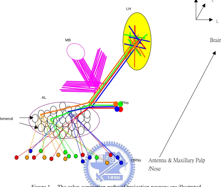
Figure 1. The calyx connection paths of projection neurons are illustrated. 3

Figure 2. Six calyxes examples are shown. 6

Figure 3. The flowchart of image-processing steps in this study is shown. 8

Figure 4. The flowchart of denoising and morphological operation is combined with median filter, closing filter, Gaussian smoothing filter and thresholding.

11

Figure 5. The T-shape skeleton is illustrated. 14

Figure 6. Two skeleton examples of two calyx data are shown, where one is noisier than the other one.

15

Figure 7. An example of terminal of end point is illustrated. 15

Figure 8. Estimated marginal means on rotational endpoints of six calyx is shown. 16

Figure 9. An example of object labeling is shown. 17

Figure 10. Estimated Marginal means on rotational objects of six calyx is shown. 18

Figure 11. An example of the separated terminals in LH is shown. 20

Figure 12. Support plane for 2 classes is demonstrated. 24

Figure 13. The SNR results of rotational images are shown. 27

Figure 14. The PSNR results of rotational images are shown. 27

Figure 15. The skeleton examples of six calyxes are shown. 29

Chapter 1. Introduction

Exploring the function of brain structure has been the long-term research topic in scientific investigation. Two modern fundamental principles of functional mechanisms in brain are functional integration and specialization, derived from connectionism and

localizationism in 19th century respectively [4]. Neuron pathway of olfactory function has

been a research topic of rising interests, especially after the pioneering studies of Richard Axel and Linda B. Buck, the Nobel Prize winner of Physiology or Medicine in 2004, for their discovery of “ordant receptors and the organization of the olfactory system”.

Fruit fly, Drosophila, is an ideal experimental model for brain research. The improvements of 3-D imaging technique on Drosophila developed by NTHU Brain Research Center provide high-resolution images [12]. It is challenging to develop automatic methods for pattern recognition of the resulting fly images. This study will investigate analysis methods for feature extraction and pattern classification on Drosophila’s olfactory pathways from 3D brain images generated by Professor Ann-Shyn Chiang at NTHU Brain Research Center.

Chapter 2. Motivation and Data Description

2.1. Research Goals

The main study purpose is the application of a classification method to determine the raw images into six categories automatically. Here we have six categories of raw images of connectivity in Drosophila olfactory neuron pathway or track(Calyx). There are two important olfactory nucleuses after Antenna Lobe (AL), Mushroom Body (MB) and Lateral Horn (LH) on the path from nose to brain. All are specified imaging of Calyx (olfactory neuron path way from glomeruli in AL to LH) [1, 3, 9, 13, 14, 17, 20, 21]. The terminologies and abbreviations of these anatomy parts are listed as following table.

ORN Olfactory Receptor Neuron

PN Projection neuron

AL Antennal Lobe

OB Olfactory Bulb; Glomeruli in side

MB Mushroom Body

LH Lateral Horn

Table 1. The biological terminologies and the corresponding abbreviations used in this study are listed.

D

Figure 1. The calyx connection paths of projection neurons are illustrated.

The projection neuron is responsible to transmitting neuron impulse to higher level in

Drosophila’s central nerve system. The main destination of projection neuron is mainly

Mushroom Body (MB) and Lateral Horn (LH). And the imaging data is describing the complexity of the axon of projection neuron.

Glomeruli

Antenna & Maxillary Palp /Nose Brain ORNs MB LH AL PNs L C

2.2. Data Description

There are six different classes in this study, which are named by the glomeruli in Antenna Lobe, DL1, VL2a, DM2, DM1, DL3 and DA1. The numbers of flies are 40, 25, 22, 13, 13, and 12 respectively. These 3D images of Drosophila’s Calyx are provided by Professor Ann-Shyn Chiang at brain research center of NTHU, Taiwan (ROC). Glomeruli are grouped according to the anatomic locations of connected olfactory receptor neurons in the smelling organ in antenna and maxillary palp [1]. Referring to the grouping result of glomeruli in [1], six glomeruli in this study can be combined to 3 or 2 categories in the following table.

6 categories 3 categories 2 categories number of flies

DL1 ab ab 40 VL2a ac ac-or-at 25 DM2 ab ab 22 DM1 ab ab 13 DL3 at ac-or-at 13 DA1 at ac-or-at 12 Total 125

Table 2. The numbers of flies in 6 categories are listed, which can be combined as 3 or 2 categories.

In each 3D image, there are three channels, red, green and blue. We will select the green channel as target information of calyx. The green channel is 8-bit depth, so the gray intensity of each voxel varies from 0 to 255. Because the size of each fly varies, the field of

view (FOV), slice and slice thickness are set according to the adequacy. For each 3D image the voxel size is consistent across slices. This information is all recorded in the header of LSM file. LSM file format is similar to TIFF. Here we take one on DL1 3D image as example, the signal intensity of each voxel is recorded in a 1024×1024×64 matrix. And there is a scale-vector representing μm/ voxel in 3 orthogonal direction of FOV. In this case,

the real size of filed of view is 194.7×194.7×63 (μm3).

DL1:GH146-singlePN49.lsm

Stack Size (Voxel) Stack Size (μm) Scaling

1024×1024×64 194.7×194.7×63 0.19×0.19×1 Table 3. The data format of one set of 3D images is listed.

In these cases of this study, the number of slice varies from 50 to 81 for the individual difference in physical sizes of these 125 flies. Therefore, the thickness of each obtained 3D images varies from 49 to 80 μm.

A typical example in every class is shown in the following figure.

DA1_PN80.bmp(at) DL1_PN47.bmp(ab)

DL3_PN111.bmp(at) VL2a_PN158.bmp(ac)

DM1_PN39.bmp (ab) DM2_PN217.bmp (ab)

Chapter 3. Analysis Methods

The main study purpose is the application of statistical classification method to determine which olfactory neuron track of the six calyxes for 3D images. In this chapter, the image pre-process for noise removal will be explained before feature extraction, and the classification methods, Fisher’s LDA and SVM are utilized after feature extraction. The essential information, e.g. RST-invariant features, describing the olfactory neuron track of the six calyxes will help us construct classification methods. For example, we will consider the rotation, scaling and translation invariant (RST-invariant) features suggested in [19]. The RST-invariant features will be useful to capture the main features in different sets of fly images in this study that are taken at different orientation, size and centering. Furthermore, the other features based on skeletons [16] could be used as well. The skeletons obtained from neuron images will be useful to detect the neuron tracks and explore genuine characteristics of neuron transmission pathways in this study. At the end, the cross validation method can be applied to evaluate classification accuracies for different features and classifiers.

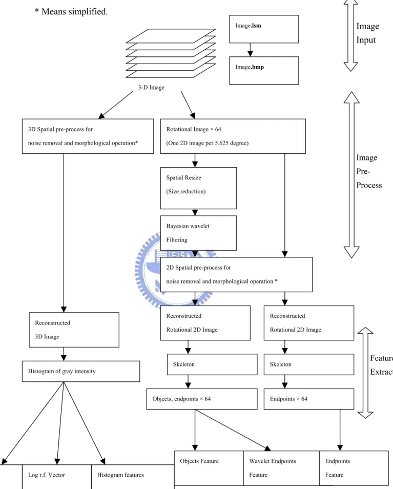
The data analysis procedures of this study are depicted in the next page based on the empiric evaluations of data in this study. The details of key steps will be explained and described in the following sections. Empirical results will be also illustrated utilizing fly neuron images in this study.

* Means simplified. Image Input Image.lsm Image.bmp 3-D Image

3D Spatial pre-process for Rotational Image × 64

(One 2D image per 5.625 degree) noise removal and morphological operation*

Image Pre-

Spatial Resize

(Size reduction) Process Bayesian wavelet

Filtering

2D Spatial pre-process for

noise removal and morphological operation * Reconstructed Rotational 2D Image Reconstructed Rotational 2D Image Reconstructed 3D Image Feature Extraction r.f. Vector

Histogram of gray intensity

Log r.f. Vector Histogram features

Skeleton Endpoints × 64 Objects, endpoints × 64 Wavelet Endpoints Feature Objects Feature Skeleton Endpoints Feature

3.1. Image Pre-Processing

Noise in physics means the fluctuations and the additional of external factors to the target information detected by any recording devices. Some degree of noise always exists in any electronic device when receiving or transmitting signals. However noise can be adjusted as relatively small to the main part of signal, and perceive as nonexistent.

Image processing of noise reduction helps recover the genuine image properties. Imperfect images with heavy noise prevent fine-clear feature extraction for further model training of pattern recognition. The purposes of noise remover consist of two key points: 1. Edges, thin lines, and small features are sharp and clean.

2. Areas between these features are smoothly varying.

Spatial filtering, spectrum filtering and morphological operations [10] will be utilized for noise reduction and feature extraction in this study. For instance, we will consider the following model for additive noise signals:

( , )

( , )

( , )

f i j

=

F i j

+

N i j

,

where f(i, j) represents the observed intensity on one 2D pixel (in the i-th row and the j-th column) and it can be composed by the unobserved signal F(i, j) with noise N(i, j). This model can be extended to signals on 3D voxels as well. Then, the following operation on the observed intensity f(i, j) can be used to recover the unobserved signal F(i, j) and its

Denoising Operation

Mean filter ] 1 , 1 [ ]; 1 , 1 [ )) , ( ( ) , ( ^ − = − = + + = b a b j a i f mean j i F Gaussian Smooth filter [ 1, 1]; [ 1, 1] )) , ( ( ) , ( ) , ( ^ − = − = + + × + + = b a b j a i f b j a i k j i F Median filter [9] ^ F ] 1 , 1 [ ]; 1 , 1 [ )) , ( ( ) , ( − = − = + + = b a b j a i f median j i Bayesian wavelet filter [15] 2 2 2 | | | ^ ^ ) ( ) ( ) ( ) ( ) ( ) | ( ) ( ) | ( ) | ( ) ( ) , ( n s s x n x n x x y x x y y x y x P x y dxP x x P x y dxP x P x y dxP x x P x y dxP x y x P dx y x j i F σ σ σ + = − − = = = =

∫

∫

∫

∫

∫

Morphological Operation

Dilation _{A B}

{

_z

[

( )

_Bˆ _A

]

_A

}

_. z∩ ⊆ = ⊕ ] 1 , 1 [ ]; 1 , 1 [ )) , ( ( ) , ( ^ − = − = + + = b a b j a i f Max j i F Erosion

_A

_B

{

_z

_B

_A

}

_.

z

⊆

=

Θ

] 1 , 1 [ ]; 1 , 1 [ )) , ( min( ) , ( ^ − = − = + + = b a b j a i f j i F Opening

_A

_o

_B

₌

(

_A

_Θ

_B

)

_Θ

_B

(

A

B

)

B

B

A

Closing

_•

₌

_{⊕ Θ}

De-isolated

points If (sum of neighbor intensity==0), replace the target pixel with zero.

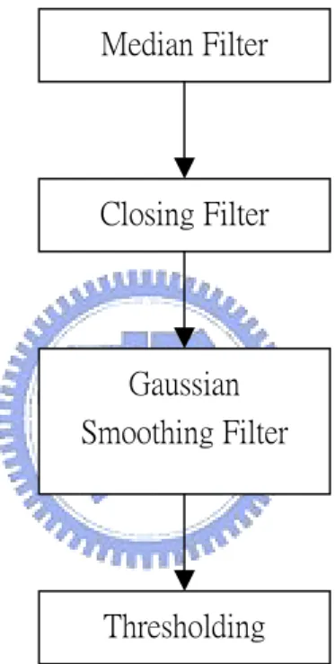
The following flowchart is the spatial pre-process for noise removal and morphological operation, which is shown simplified in Figure3 of P.8. All the operation in this flowchart

can be applied for any 3D and 2D image; the only difference is the neighbor window is 33 for

3D, and 32 for 2D. The flowchart of denoising and morphological operation is combined

with median filter, closing filter, Gaussian smoothing filter and thresholding, and they are performed in this order.

Median Filter

Closing Filter

Gaussian Smoothing Filter

Thresholding

Figure 4. The flowchart of denoising and morphological operation is combined with median filter, closing filter, Gaussian smoothing filter and thresholding.

M-1 N-1 2 0 0 M-1 N-1 ₂ 0 0 ˆF(i,j) SNR ˆF(i,j)-f(i,j) i j i j = = = = = ⎡ ⎤ ⎣ ⎦

∑∑

∑∑

.

Alternatively, there are other measures similar to SNR. For example, the peak signal-to-reconstructed image measure (PSNR) will be another considering measure. It is defined through the following procedure. First, the mean square error (MSE) is calculated. Secondly, by taking root of MSE the root mean square error (RMSE) can be derived. Thirdly, the PSNR will be calculated by twenty times of log of RMSE.

1 1 2 ( , ) ( , ) 0 ˆ ( ) M N i j i j i o j f F MSE N M − − = = − = ⋅

∑∑

MSE RMSE = ⎟ ⎠ ⎞ ⎜ ⎝ ⎛ ⋅ = RMSE PSNR 20 log₁₀ 255

Although there is not a perfect method of noise reduction, here we will utilize SNR and PSNR as referenced measures for the evaluation index.

3.2. Feature Extraction

Feature extraction will be application-dependent. In my end goal of this study is the generation of classifier for six calyx 3D images. Therefore a proposed feature extraction for retrieving distinctive representations from the 6 calyx images is required to be informative, robust, consistent and invariant. The robustness index is discussed in feature vectors and

feature space while the target object is obtained from different angles, distances, imaging settings and so on. The observed object in images resulted in different resolutions, sizes, translations and rotations. Informative features will be RST-invariant, and contributed for higher classification accuracy. In fact, if the classification accuracy with these RST-features is not computed or comparatively high, some other informative RST-features hunting should never stop. For generating the dataset for classification in this study, the RST-invariant features and rotational skeleton features are utilized. Those features are used for describing the different complexity in projection neuron’s spatial dispersions in 3D space.

3.2.1. RST-invariant Feature

The two-dimensional image processes for RST-invariant feature extraction is discussed in the frequency and the spatial domains [19]. For a binary images object features can be area, center of area, and the axis of least second moment, perimeter, Euler number, projections in row or column, thinness ratio, and aspect ratio. The first four tell us location of the object in image, and the last four tell us the shape of the object. For gray images, histogram features are mean, standard deviation, skewness, energy, and entropy. The strength of these RST-invariant features is robustness with the object in image is rotated, adjusted in size, which means diminishing or enlarging in area, and shifted left/right or up/down.

1. Skeleton

Skeletonizing is also called thinning in morphological operation. In binary images, by peeling of the boundary pixels, the skeleton of the object left keeps the features, pattern and shape. Many skeleton algorithms have been well developed [5, 7, 8, 18, 22].

The skeleton of object set A by structure set B is defined as the following set operations,

) ) ) (((A B B B kB AΘ = Θ Θ ⋅ ⋅⋅Θ B kB A kB A A Sk( )=( Θ )−( Θ )o

U

∞₌ = 0 ) ( ) ( k k A S A S

Skeletonization operation of A by B iterates for k times. The stop criterion is until no any pixel is deleted. S(A) is the skeleton of A. The obtained skeleton must have three properties:

1. Connected for any single object. 2. As thin as possible.

3. The skeleton is in the middle axis.

The idea of skeleton is shown in the following figure.

● ● ● ● ● ● ● ● ● ● ● ● ● ● ● ● ● ● ● ● ● ● ● ● ● ● ● ● ● ● ● ● ● ● ● ● ● ● ● ● ● ● ● ● ● ● ● ● ● ● ● ● ● ● ● ● ● ● ● ● ● ● ● ● ● ●

Set A: a T-shape object S(A): the skeleton of T-shape object Figure 5. The T-shape skeleton is illustrated.

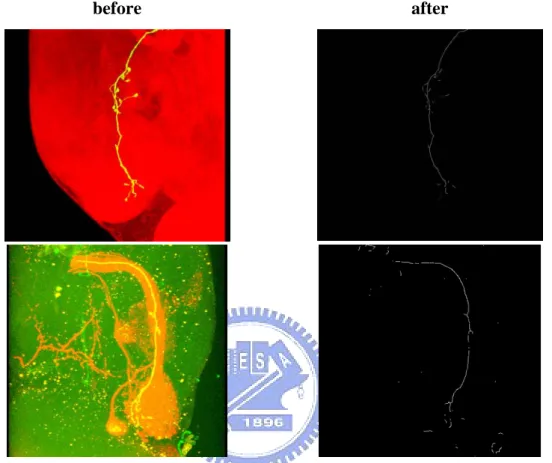
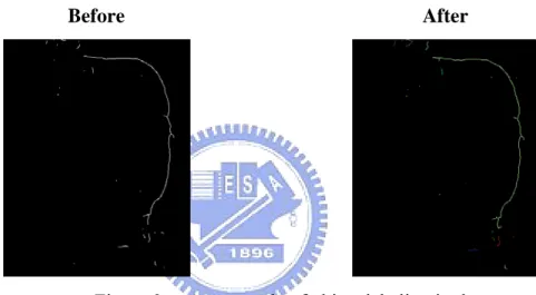
For this empirical data in this study, we utilize the integrated procedure of Stentiford preprocessing [18], Z-S algorithm [22] and Holt algorithm [9]. The effect of implementation of skeleton procedures after pre-process is demonstrated in the following figure.

before after

Figure 6. Two skeleton examples of two calyx data are shown, where one is noisier than the other one.

2. Endpoints

Any one and only one of the target 2D pixel’s eight neighbors has non-zero intensity, and the target pixel is an endpoint. An example of endpoint is show above. Here the pixel with non-zero intensity, while only one of its eight neighbors has non-zero intensity.

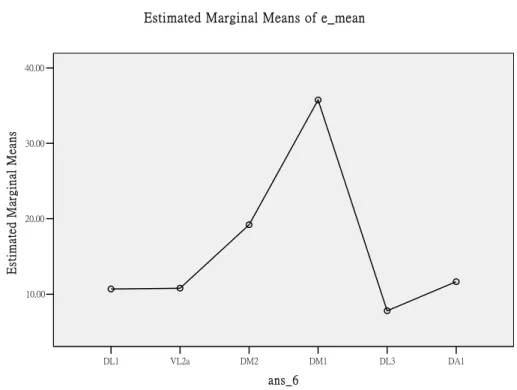
Here the endpoint of calyx means a terminal spot in the olfactory neuron path. The number of endpoints means the number of terminal spot in the olfactory neuron path, while the fly’s neuron system transmitting information upward to brain after antennal lobe. In the following ANOVA table, the mean number of rotational endpoints is significantly different across six categories with the p-vale=0.000.

Tests of Between-Subjects Effects Dependent Variable: e_mean

7963.633a _{5 1592.727 15.979 .000} 26460.491 1 26460.491 265.463 .000 7963.633 5 1592.727 15.979 .000 11861.542 119 99.677 46506.232 125 19825.176 124 Source Corrected Model Intercept ans_6 Error Total Corrected Total

Type III Sum

of Squares df Mean Square F Sig.

R Squared = .402 (Adjusted R Squared = .377) a.

Table 5. ANOVA table of six calyx on mean of rotational endpoints is shown.

DA1 DL3 DM1 DM2 VL2a DL1 ans_6 40.00 30.00 20.00 10.00 Es timate d Marginal M eans

Estimated Marginal Means of e_mean

Figure 8. Estimated marginal means on rotational endpoints of six calyx is shown.

categories. DM1 it is the category with high complexity comparing to the other 5 categories, and DM1 has the satisfactory highest mean in the rotational endpoints feature.

3. Region growing for object labeling

After these pre-processing and skeletonization, the main stem skeleton is remained, while there are some separated pieces remaining. The positions of endpoints are set to be the initial seed for region growing labeling. When the growing labeling meets, it will be merged to be a single object with the same label.

Before After

Figure 9. An example of object labeling is shown.

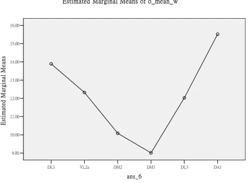
There are six separated objects including the main stem in this image; these unconnected objects are shown with different colors. For the calyx in 3D space, there will be 64 rotational projection views. The number of separated objects varies from different views of angle. The number of objects describing the small pieces derived from main stem in MB and LH. The mean number of separated objects is significantly

Tests of Between-Subjects Effects Dependent Variable: o_mean_w

475.769a 5 95.154 3.292 .008 15266.198 1 15266.198 528.152 .000 475.769 5 95.154 3.292 .008 3439.684 119 28.905 23018.220 125 3915.453 124 Source Corrected Model Intercept ans_6 Error Total Corrected Total

Type III Sum

of Squares df Mean Square F Sig.

R Squared = .122 (Adjusted R Squared = .085) a.

Table 6. The ANOVA table of six calyxes on mean of rotational objects is shown.

DA1 DL3 DM1 DM2 VL2a DL1 ans_6 16.00 15.00 14.00 13.00 12.00 11.00 10.00 9.00 Est im ate d Ma rg in al M ean s

Estimated Marginal Means of o_mean_w

Figure 10. Estimated Marginal means on rotational objects of six calyx is shown.

Here these features can be grouped in 4 groups.

1. Relative frequency (r.f.) vector and log r.f. vector of intensity histogram

Relative frequency vector of intensity histogram is the simple statistics of this 3-D image with gray intensity (integer) from zero to 255. Since the total number of

pixels is very large, some element of r.f. Vector has a value very small, even close to zero. It might be hardly to distinguish the subtle difference between six calyx categories. Here the log transformation is utilized.

2. Histogram features

There are six features generated by intensity histogram, mean intensity, S.D. of intensity, skewness and kurtosis of intensity histogram, number of nonzero pixel, energy and entropy.

3. Rotational skeleton endpoints features

The 64-sliced rotational 2D projection images are utilized for representing the 3D calyx image. For each 2D image of the 64 in a set, we run 2D denoising process and skeletonization. At last, only the largest object, which is the skeleton of calyx, will be remained. The 64-sliced rotational 2D skeleton represents the 3D calyx from 64 different angles in a circle. For each 3D calyx, we can calculate endpoints in 64 2D skeletons from 64 different angles in a circle. For the same category of calyx, there is a hypothesis; the distribution of rotational endpoints should be very similar but different across different categories. The number of endpoints is viewed as a random variable, and the observed number of endpoints from different angles is the obtained data. Therefore we will calculate the 4 moments of the number of endpoints as endpoints moment feature and the 10%-increased percentiles as endpoints percentile

especially in LH and MB. And here we will count the number of endpoints in the main stem only.

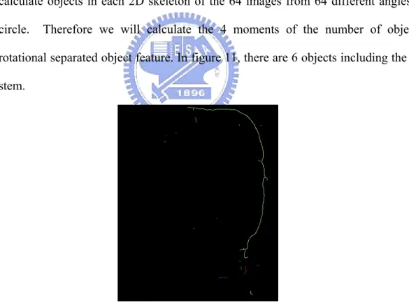
4. Wavelet objects feature

For each 64-sliced rotational projection 2D image sets, the utilization of spatial size reduction in pixel and Bayesian Wavelet Filtering (BLS-GSM) [15] will be done before the 2D pre-processing and skeletonization. The wavelet skeleton tends to have terminal pieces separated from the main stem especially in LH and MB on these calyx image data. Therefore, we will use object labeling to calculate how many separated objects including the main stem in a 2D image. For each 3D Calyx, we can calculate objects in each 2D skeleton of the 64 images from 64 different angles in a circle. Therefore we will calculate the 4 moments of the number of object as rotational separated object feature. In figure 11, there are 6 objects including the main stem.

Code in Classification

Model

Description Number of

attributes

F1 Rotational Endpoints Moment Feature 4

F1** Rotational Endpoints Percentile Feature 11

F1* Wavelet R. Endpoints Feature 4

F2 Rotational Object Feature 4

F3 Relative frequency (r.f.) vector 256

F3* Log r.f. vector 256

F4 Histogram Feature 7

Table 7. The Features Code is listed.

The combination of selection of feature groups for classifier can be interpreted as a statistical problem, which is known as model selection. The possible combination will be

25*2 rather than 27, for F3 and F3*, only one of them will be selected in a model. For the

possible combinations can too many choices, here I will run 26 different combinations of interest.

3.3. Classification

The terminologies of some concepts in statistics are quite different from computer science. Terminology of predicting a discrete Y from X is classification in statistics and supervised learning in computer science. The comparison of these terminologies atr listed in the following table.

Statistics Computer Science Meaning

Classification Supervised learning Predict a discrete Y from X

Data Training sample (X1, Y1), …, (Xn, Yn)

Covariates Features The Xi’s

Classifier Hypothesis Map h: X→Y.

Estimate Learning Using data to find an unknown quantity,

finding a good classifier

Table 8. Terminologies in CS and statistics are compared here.

This The Xi’s in training samples are covariates in statistics and features in computer science.

(X1, Y1),…, (Xn, Yn)

where X is a d-dimensional vector and Yi takes values in a finite

set Y.

∈

=(X ,...,X )

X_{i i1 id} ⊂ℜd

A classification rule is a function h: X→Y. When we have a new query Xn+1, we predict

Yn+1 to be h(Xn+1).

There are many ways to estimate error rates and it helps us at choosing a good classifier. We will consider cross-validation. The data are divided into two groups, training setτ and

we apply into the validation set for the estimation of the error rate . h^ ^ L

∑

∈ ≠ = ν i X i i Y X h I m h L( ) 1 ( ( ) ) ^

, where m is the size of ν .

Leave-one-out validation will be useful for the error rate estimate. Here two different classifiers, LDA and SVM, are introduced briefly in the following sections.

3.3.1. Fisher Linear Discriminant Analysis (LDA)

Fisher’s LDA is a classification method. LDA project dataset in

onto a one-dimensional space, and the classification is performed on the projection line. The mean vectors and variance matrixes of the two different classes decide the projection line. This projection maximize the distance between the mean points of two different classes, while the within variances of each class is minimized [2]. In this study, SPSS13.0 “classify>Discriminant” is utilized for the results of Fisher’s LDA.

) ,...,

( i₁ id

i X X

X = ℜd

3.3.2. Support Vector Machine (SVM)

SVM [11] is another kind of supervised learning methods used for classification, and it is also a generalized linear classifier. The basic idea is how to map our data/ observations into a higher dimensional space and find out the maximal separation/gap between different classes. The goal of SVM is to find out the optimal hyper-plane (maximal margin hyper plane) which

Figure 12. Support plane for 2 classes is demonstrated.

ω·x-b=0 ω·x-b=1

ω·x-b=-1

w

2

∈ =( _i1,..., _id) i X X

X X ⊂ℜd is a d-dimensional vector, and ω is the normal vector of

the maximal margin hyper plane. Here we have ω·x-b=0 as the dividing hyper plane. Therefore, we describe the two parallel hyperplanes closest to these support vectors in either class with following equations.

⎩ ⎨ ⎧ − = − ⋅ = − ⋅ 1 1 b x b x ω ω

Hence, for each X_i, , and there is no any fall within the separation.

⎩ ⎨ ⎧ − ≤ − ⋅ ≥ − ⋅ 1 1 b x or b x i i ω ω i X

w

2

And our focus interest is on the maximal margin , so we can

min ω , subject to c_i(ω⋅x_i −b)≥1, ∀i=1,2,...,n

For mathematical convenience, we will transform the original problem to a quadratic programming (Q-P) optimization, 2 2 ω , subject to min ci(ω⋅xi −b)≥1, ∀i=1,2,...,n

The Dual form of SVM classifier decided by the support vectors, i.e. the training dataset that lie on the boundary. The dual form of the SVM can be shown as:

∑

∑

= − n i i j j T i j i j i i cc x x 1 , max α αα subject toα_i ≥0, ∀i=1,2,...,n where the i

α

~

constitute a dual representation for the weight vector in terms of the training dataset:

∑

= i i i ic x α ω

Although we endure ξi≧0, the penalty is defined as

∑

. And we will need to

minimize the penalty with the Q-P optimization

= n i i 1 ξ 2 2 ω

. Therefore, the revised equation is:

∑

+ i i C w 2 ξ , subject to min ci(ω⋅xi −b)≥1−ξi, ∀i=1,2,...,n

Here we are going to utilize SMO in WEKA for the result with SVM.

Chapter 4 Results

In this chapter, the reconstructed images of six calyxes (olfactory neuron track of

Drosophila) are checked with SNR and PSNR. And the accuracies of different classification

models with various feature combinations are also reported. Similar to regression method, the model selection here means the selection of classification method and selection of feature combinations. R-square or adjusted R-square can be helpful index for regression model, and the cross validation accuracy is our evaluation index to determine the superior method of classifying six different calyxes.

4.1.

SNR PSNR and Skeleton Image

The SNR and PSNR of reconstructed images fluctuate, but the image quality is generally improved. Because the skeleton operation is very sensitive to noise, the pre-process of rotational images are carefully considered. As our expectation, most of the reconstructed images has SNR greater than 1.0, and PSNR within 20 to 40. And the s.d. of SNR and PSNR of rotational images are also checked. The improved image quality doesn’t fluctuate greatly across and within categories.

DA1 DL3 DM1 DM2 VL2a DL1 ans_6 2.5 2.0 1.5 1.0 0.5 0.0 95% C I w_SNR_sd w_SNR_mean

Figure 13. The SNR results of rotational images are shown.

DA1 DL3 DM1 DM2 VL2a DL1 ans_6 40 30 20 10 0 95% C I w_PSNR_sd w_PSNR_mean

After the image process, all the 3D Calyx images are simplified as rotational skeleton. Skeletons of six calyxes are varying differently in the complexity of the spatial dispersion. The 64-sliced rotational image describes the axon of projection neuron in 3D space, and the 64-sliced rotational skeleton is the simplified version of the calyx.

DA1_PN80.bmp(at)

DL1_PN47.bmp(ab)

DM1_PN39.bmp(ab)

DM2_PN217.bmp(ab)

VL2a_PN158.bmp(ac)

Figure 15. The skeleton examples of six calyxes are shown.

4.2. Accuracy

model feature code #of attributes LDA_2 LDA_3 LDA_6 SVM_2 SVM_3 SVM_6

1 F1 4 64 48 36.8 59.2 60 31.2 2 F2 4 56 38.4 28 60 60 32 3 F1* 4 48.8 29.6 16 60 60 32 4 F4 7 71.2 60.8 42.4 60 60 40.8 5 F1+F2 8 53.6 42.4 33.6 60 60 32 6 F1+F4 11 72.8 57.6 44.8 68.8 60 39.2 7 F1*+F2+F4 15 64.8 50.4 40 58.4 60 40.8 8 F1+F2+F4 15 66.4 59.2 40.8 63.2 61.6 44 9 F1+F1** 15 62.4 45.6 29.6 58.4 60 40 10 F1*+F2+F4+F1 19 64 55.2 44.8 67.2 60.8 45.6 11 F1+F1**+F4 22 69.6 57.6 43.2 67.2 61.6 48.8 12 F1+F1**+F3*+F4 26 70.4 62.4 47.2 76 71.2 53.6 13 F3 256 73.6 64 44 66.4 62.4 43.2 14 F3* 256 72 60 39.2 76.8 67.2 52.8 15 F3+F4 263 71.2 61.6 42.4 68.8 64.8 44 16 F3*+F4 263 68 64 42.4 80 72 52.8 17 F3+F4+F1 267 72 61.6 42.4 70.4 61.6 45.6 18 F3*+F4+F1 267 68.8 64 42.4 79.2 69.6 54.4 19 F3+F4+F2 267 68.8 64.8 41.6 70.4 62.4 48 20 F3*+F4+F2 267 66.4 64 44 80 70.4 50.4 21 F3+F4+F1+F2 271 68.8 64.8 42.4 68 62.4 47.2 22 F3*+F4+F1+F2 271 66.4 64 44 80 71.2 52.8 23 F3+F4+F2+F1* 271 65.6 64.8 42.4 71.2 63.2 46.4 24 F3*+F4+F2+F1* 271 68 64 37.6 79.2 71.2 52.8 25 F1+F3+F4+F2+F1* 275 64.8 64.8 42.4 70.4 61.6 47.2 26 F1+F3*+F4+F2+F1* 275 70.4 64 39.2 79.2 70.4 52.8

Table 9. Table of Leave-one-out Accuracy of 26 interested models is shown.

First, the accuracy of SVM is generally better than LDA across the 23 different feature combinations. SVM outperforms LDA, for the over-simplification of mapping function of LDA on one-dimension, while SVM is finding a max-margin separation hyper-plane on sample space. The subtle difference across six categories are delimitated by LDA.

accuracy 0 10 20 30 40 50 60 70 80 90 1 2 3 4 5 6 7 8 9 10 11 12 13 14 15 16 17 18 19 20 21 22 23 24 25 26 LDA_2 LDA_3 LDA_6 SVM_2 SVM_3 SVM_6

times of random guess

0 0.5 1 1.5 2 2.5 3 3.5 LDA_2 LDA_3 LDA_6 SVM_2 SVM_3 SVM_6

validation accuracy, 54.4%. The random guess rate is one divided by the number of categories. Here for six- category classifier, the random guess rate is 1/6. And all the

accuracy should be divided by the random guess rate. In the 18th model, the accuracy is higher

than random guess rate more than 3 times. Rotational skeleton Endpoint feature helps the

six-category- SVM classifier with log r.f. vector and histogram feature in the 18th model.

Chapter 5 Discussion

For human beings, comparing to the dominant vision, the functional connection beyond glomerulus for the smelling chemicals remain a mysterious story. In Drosophila, the two important nucleuses in neuron pathway going beyond the well-studied AL are LH and MB. And for each glomerulus in AL, the further pathway going upward to brain is basically called Calyx. For the Calyx 3D imaging, it can be perceived as 3 main parts, the main stem, MB and LH. For each partition, there is a gray intensity histogram. These three parts mainly compose the intensity histogram of the whole gray 3D image. And the produced rotational skeleton of Calyx is mainly a simplified functional connection version. And those utilized features describe the dispersion of neuron signal transmitting of Drosophila; especially the endpoints feature and object features. The complexity of the functional connection for different smelling senses is very fascinating for many neuron biologists. The consummating discovery of the olfactory perception mechanism is still waited to be finished. Therefore, there are several directions for us keeping work on further improvement the accuracy.

First, while the corrupting noise is always inevitable for any imaging equipments, better denoising image preprocess might raise the quality of reconstructed images, especially the sensitivity to noise of the skeleton operation is known for us. Secondly, the applications of better 3D alignments and spatial partition of main stem, MB and LH before some more 3D RST invariant and other features and more tuning of classification methods will contribute as

a pilot study for the accomplishment of Hidden Markov Model and Fractal Analysis in the future. Third, the further application at integrated reconstruction from the rotational 2D skeleton to 3D skeleton may play a possible heuristic idea for 3D skeleton operation.

Besides, some more possible biological extended applications of the results of this study at fly, Drosophila, to human or other species are also potential future works.

Reference

[1] Africa Couto, Mattias Alenius, and Barry J. Dickson, “Molecular, Anatomical,

and Functional Organization of the Drosophila Olfactory System.” Current Biology, Vol 15, 1535-1547, 06 September 2005.

[2] Fisher, R.A. “The Use of Multiple Measurements in Taxonomic Problems”.

Annals of Eugenics, 7: 179-188,1936.

[3] Fishilevich, E., Vosshall, L.B. “Genetic and functional subdivision of the

Drosophila antennal lobe”. Current Biology 15(17): 1548--1553, 2005.

[4] Freeman, Walter J., “The Physiology of Perception.” Scientific American, Vol.

264, (2) Page 78-85., 1991.

[5] R. Fabbri, L.F. Estozi and L. da F. Costa. “On Voronoi Diagrams and Medial

Axes”. Journal of Mathematical Imaging and Vision, 17(1), Pages 27-40, July 2002.

[6] Gregory SXE Jefferis, Elizabeth C Marin, Ryan J Watts and Liqun Luo,

“Development of neuronal connectivity in Drosophila antennal lobes and mushroom bodies,” Current Opinion in Neurobiology, 12:80–86., 2002.

[8] Holt, C. M., Stewart, A.,Clint, M. and R.H. Perrott. “An Improved Parrallel Thinning Algorithm”. Communications of the ACM, 30(2):156-160. 1987.

[9] T.S. Huang, G.J. Yang and G.Y. Tang. “A fast two-dimensional median filtering

algorithm”, IEEE Transactions on Acoustics, Speech and Signal Processing, vol.27, pp13-18, 1979

[10] C. Jeremy Pye and J.A. Bangham. “A Fast Algorithm for morphological Erosion

and Dilation”

[11] Joachims, T., “Text categorization with support vector machines: Learning with

many relevant features”, In Proceedings of the European Conference on Machine Learning. Springer, 1998.

[12] Lin HH, Jason Lai SY, Chin AL, Chen YC, Chiang AS. “A Map of Olfactory

Representation in the Drosophila Mushroom Body”. Cell 128, 1205-1218, 2007.

[13] Elizabeth C. Marin, Gregory S.X.E. Jefferis, Takaki Komiyama, Haitao Zhu,

“Representation of the Glomerular Olfactory Map in the Drosophila Brain,” Cell, Vol. 109, 243–255, April 19, 2002.

[14] Marien de Bruyne, Kara Foster and John R. Carlson, “Odor Coding in the

Drosophila Antenna,” Neuron, Vol. 30, 537–552, May, 2001,

[15] J Portilla, V Strela, M Wainwright, E P Simoncelli. “Image Denoising using

Scale Mixtures of Gaussians in the Wavelet Domain”. IEEE Transactions on Image Processing. vol 12, no. 11, pp. 1338-1351, November 2003.

[16] Parker, J. R. “Algorithm for Image Processing and Computer Vision”, Wiley

Computer Publishing, 176-188, 1999.

[17] Rajesh Ranganathan and Linda B. Buck, “Olfactory Axon Path finding: Who Is

the Pied Piper?” Neuron, Volume 35, Issue 4, 15, Pages 599-600 ,August 2002.

Handprinted Charaters for OCR”. IEEE Transactions on Systems, Man and Cybernetics. 13(1):81-84, 1983.

[19] Scott E. Umbaugh, Yansheng Wei and Mark Zuke, “Feature Extraction in Image

Analysis,” IEEE Enginneering in Medicine and Biology, July/August, 1997.

[20] Vosshall LB, Wong AM, Axel R., “An olfactory sensory map in the fly brain.”

Cell. 2000 Jul 21;102(2):147-59.

[21] C. Ron Yu, Jennifer Power, Gilad Barnea, Sean O'Donnell, Hannah E. V.

Brown, Joseph Osborne, Richard Axel and Joseph A. Gogos, “Spontaneous Neural Activity Is Required for the Establishment and Maintenance of the Olfactory Sensory Map,” Neuron, Volume 42, Issue 4, 27 May 2004, Pages 553-566

[22] Zhang, S. and K.S. Fu., “A thinning Algorithm for Discrete Binary Images”.

Proceedings of the International Conference on Computers and Application. Beijing, China. 879-886,1984.