國 立 交 通 大 學
電信工程學系碩士班
碩 士 論 文
以偽貝氏廣播為基礎的媒體存取控制之協定
A Pseudo-Bayesian-Broadcast-Based MAC Protocol
研 究 生:林國瑋 Student:
Kuo-Wei
Ling
指導教授:廖維國 博士 Advisor:
Dr.
Wei-Kuo
Liao
以偽貝氏廣播為基礎的媒體存取控制之協
定
A Pseudo-Bayesian-Broadcast-Based MAC Protocol
研 究 生:
林國瑋
Student:
Kuo-Wei Ling
指導教授:廖維國 博士 Advisor:
Dr.
Wei-Kuo
Liao
國 立 交 通 大 學
電信工程學系碩士班
碩 士 論 文
A Thesis Submitted to
the Department of Communication Engineering
College of Electrical and Computer Engineering
National Chiao Tung University
in Partial Fulfillment of the Requirements
for the Degree of Master of Science
In
Communication Engineering
July 2008
以偽貝氏廣播為基礎的媒體存取控制之協
定
研 究 生:
林國瑋
指導教授:廖維國 博士
國 立 交 通 大 學
電信工程學系碩士班
中文摘要
估計出參與在無線通訊系統中,想要重送封包的使用者數目,對於提升某些分散式 媒體存取控制協定系統的效能,是特別重要的。為了解決這個困難的問題,Rivest 提出 偽貝氏演算法,在穩定的時槽式 Aloha 系統中,可以不需要知道使用者的數目,簡單又 有效地解決上述的問題。他的運作方式是藉由保持住,在每一個時槽開始時,要重送的 使用者的估計值。在這篇論文裡,我們著重在以時槽式 Aloha 為基礎的分散式媒體存取 控制之協定中,維持要重送的使用者個數的估計值。最基本的協定形式是從穩定的 Aloha 開始,接著如果發生某些情況,則系統進入第二模式,第二模式是一個縮短的樹狀分裂 的演算法。今過一段有限的時間後,系統會重新回到穩定的 Aloha 模式下。第二模式是 一個提高效能的模式。如同 Rivest 的偽貝氏演算法,我們提出一個方法,可以不需要 知道使用者的個數,並且提高有效傳輸量。中華民國九十七年七月
A Pseudo-Bayesian-Broadcast-Based MAC Protocol
Student:
Kuo-Wei Ling
Advisor: Dr. Wei-Kuo Liao
Department of Communication Engineering
National Chiao Tung University
Abstract
Estimating the number of backlogged users participating in wireless communications is particularly important for enhancing the performance of some distributed MAC protocols. To resolve such a difficult issue, Rivest’s Pseudo- Bayesian algorithm is a simple and effective way to doing so in stabilized slotted aloha without knowledge of the number of nodes. It operates by maintaining an estimate of the backlogged user at the beginning of each slot. In this thesis, we focus on estimating the number of backlogged users for the slotted-aloha-based distributed MAC protocols. A basic form of these protocols is starting from the stabilized aloha and then if certain condition occurs, the system goes to second mode which is indeed a truncated tree splitting algorithm. After a finite period, the system moves back to the mode of stabilized aloha. The second mode could be a performance boost mode. As in Rivest’s Pseudo-Bayesian algorithm, our proposal does not require the acknowledgement of the number of nodes, and increase the throughput.
誌謝
首先誠摯的感謝我的指導教授廖維國老師,老師淵博的學問及悉心的指導,使我獲 益匪淺,老師及師母對我的幫助,我永記於心。其次感謝張文鐘老師及田伯隆老師,百 忙中抽空擔任我的口試委員,並給我寶貴的指導與建議。 還要感謝柯柯,賢宗,俊宏,天書,Baku,葉公子,阿中,搞弟,給我學業或是 生活上的幫助。感謝永裕,Kemp,郁媛,Oga,所有的 812B 成員,因為有你們讓實驗 室充滿了歡笑,是我過了許久仍回味無窮的珍貴回憶。 另外還要感謝我的舅舅,鼓勵我,使我遇到困難學會勇敢面對,不逃避問題, 感謝我的好友淑賢,德揚,家豪,雅文,橄欖,李萱,感謝妳們ㄧ路陪伴我走過痛 苦或是快樂的日子。 最後,謹以此文獻給我摯愛的母親。Contents
Chinese Abstract……….. iii
English Abstract………... iv Acknowledgment……….. v Contents………. vi List of Figures………vii List of Tables………..viii Chapter 1 Introduction………. 1
Chapter 2 Background Knowledge……….. 3
2.1 Slotted Aloha……… 3
2.2 Pseudo-Bayesian algorithm………. 7
2.3 Splitting Tree Algorithms………. 13
Chapter 3 A Pseudo-Bayesian-Broadcast-Based MAC Protocol……… 16
3.1 Model……….. 16
3.2 A Pseudo-Bayesian-Broadcast-Based MAC Protocol………. 17
3.3 Estimate
nˆ
algorithm………. 24Chapter 4 Throughput analysis………... 26
Chapter 5 Simulator and simulation results………... 30
5.1 Simulator……….. 30
5.2 Simulation results……… 32
Chapter 6 conclusion………. 37
List of Figures
Fig. 2.1 Departure rate as a function of attempted transmission rate G for slotted
Aloha………4
Fig. 2.2 Markov chain for slotted Aloha……….. 5
Fig. 2.3 Instability of slotted Aloha……….. 6
Fig. 2.4 Tree algorithm……….. 13
Fig. 3.1 CRP time one transmission successes. CRP time period is 1…………... 18
Fig. 3.2 CRP time one transmission feedback is idle. CRP time period is 1... 19
Fig. 3.3 CRP time one transmission feedback is collision. And CRP time 2 transmission feedback is idle. CRP time period is 3………...……... 21
Fig. 3.4 CRP time one transmission feedback is collision. And CRP time 2 transmission feedback is success (1). CRP time period is 3………... 22
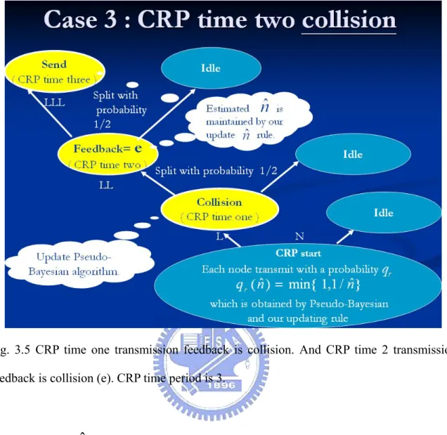
Fig. 3.5 CRP time one transmission feedback is collision. And CRP time 2 transmission feedback is collision (e). CRP time period is 3……….…. 24
Fig. 4.1 One nodes split to the left subset when a CRP starts…….……… 27
Fig. 4.2 k≥2 nodes split to the left subset when a CRP starts and CRP time 2 feedback is 0……….……….…... 28
Fig. 4.3 k≥2 nodes split to the left subset when a CRP starts and CRP time 2 feedback is 1……….………..……... 28
Fig. 4.4 k≥2 nodes split to the left subset when a CRP starts and CRP time 2 feedback is e………...………… ………..……… 29
Fig. 5.1 OMD of the Simulator……… ………..………… 31
Fig. 5.2 State Chart of “nodegenerator”……….……….. 31
Fig. 5.3 State Chart of “channel”……….……….. 31
Fig. 5.4 Arrival rate=0.1………..……… 32
Fig. 5.6 Arrival rate=0.3……… 33
Fig. 5.7 Arrival rate=0.4……… 33
Fig. 5.8 Arrival rate=0.41……….………. 33
Fig. 5.9 Arrival rate=0.42……….………. 33
Fig. 5.10 Arrival rate=0.43………. 33
Fig. 5.11 Arrival rate=0.99………. 33
Fig. 5.12 Average delay time vs. arrival rate……… 34
Fig. 5.13 Throughput vs. arrival rate……….….…….. 34
Fig. 5.14 Average delay time vs. arrival rate (0.1~0.99)……….….……. 35
Fig. 5.15 Throughput vs. arrival rate (0.1~0.99)……….….………. 36
List of Tables
Table 5.1 The average delay and throughput for each arrival rate, and simulation 106 time slot……….……… 35Table 5.2 The average delay and throughput for each arrival rate, and simulation 105 time slot………..……… 36
Chapter 1
Introduction
Estimating the number of active or so-called backlogged users participating in wireless communications is of particularly important for enhancing the performance of some distributed MAC protocols. For example, in slotted aloha, a distributed MAC protocol in use in satellite and radio communication for data transfer, packets are transmitted by various users. More packets sent simultaneously indicate a collision. To enhance the throughput of slotted aloha, the stabilized slotted aloha sets the transmission probability of sending a backlogged packet as 1/n, where n is number of backlogged users which have backlogged packets to send. It has been shown that the stabilized slotted Aloha can achieve the maximum throughput of slotted aloha. Due to the nature of distributed system, however, such a number n can only be estimated by observing the channel utilization and the corresponding feedback.
To resolve such a difficult issue, Rivest’s Pseudo-Bayesian algorithm is a simple and effective way without knowledge of the number of nodes. It operates by maintaining an estimate nˆ of the backlog n at the beginning of each slot. Both new arrival and backlogged packets are transmitted with probability qr(nˆ)= ,1}
ˆ 1 min{
n . The estimated backlog at the
beginning of slot k+1 is updated from the estimated backlog and feedback for slot k. The maxima throughput in this algorithm is 1/e, which has been proved to be the maximum throughput of slotted aloha system.
protocols. A basic form of these protocols is starting from the stabilized aloha and then if certain condition occurs, the system goes to second mode. After a finite period, the system moves back to the mode of stabilized aloha. The second mode could be a performance boost mode. For example in [1], the second mode is indeed a truncated tree splitting algorithm, which is an approach that divides the users involved in a collision into several subsets using some tree like mechanism [1]. With such two modes, not only the performance can be improved to the maximum throughput in the tree splitting algorithm, which is about 0.43, but also the robustness against the inconsistent view of current tree evolution is also improved.
As in Rivest’s Pseudo-Bayesian algorithm, our purpose is to find an algorithm that does not require the acknowledgement of the number of nodes, and increase the throughput. In our thesis, for the second mode we also consider a splitting algorithm. However, our version of splitting algorithm does not include the common receiver and thus doing so renders it more applicable to wireless access system. Using our method is to estimate nˆ of the backlog n by receiving the feedback and to combine our splitting algorithm police to reduce collision. Finally, the throughput by using our policy is 0.423.
The rest of the thesis is organized as follows. In chapter 2 we introduce the background knowledge of our study. The system framework is presented in chapter 3. And the analysis of “A Pseudo-Bayesian-Broadcast-Based MAC Protocol” is described in chapter 4. Briefly describe our simulator and then simulation results are reported in chapter 5, followed by conclusion in chapter 6.
Chapter 2
Background Knowledge
In this chapter, we will introduce the basic idea of slotted Aloha, Pseudo-Bayesian algorithm, and tree-splitting Algorithm.
2.1 Slotted Aloha
Slotted Aloha, which introduced discrete timeslots. The basic idea of this algorithm is that each unbacklogged node simply transmits a newly arriving packet in the first slot after the packet arrival, thus risking occasional collisions but achieving very small delay if collisions are rare. When a collision occurs in slotted Aloha, each node sending one of the colliding packets discovers the collision at the end of the slot and becomes backlogged. If each backlogged node were simply retransmit in the next slot after being involved in a collision, then the other collision would surely occur. In stead, such nodes must wait for some random number of slots before retransmitting.
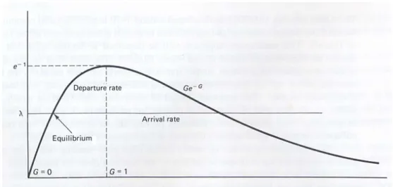
With the infinite-node assumption, the number of new arrivals transmitted in a slot is Poisson random variable with parameter λ. If the retransmission from the backlogged nodes are sufficiently randomized, it is plausible to approximate the total number of retransmissions and new transmissions in a given slot as a Poisson random variable with some parameter G > λ. With this approximation, the probability of successful transmission in a slot is Ge−G. Finally, in equilibrium, the arrival rate, λ, to the system should be the same as the departure rate, Ge−G. This relationship is illustrated in Fig. 2.1.
The maximum possible departure rate occurs at G=1 and is 1/e ≈0.368. if G < 1, too many
Fig. 2.1 Departure rate as a function of attempted transmission rate G for slotted Aloha.
Ignoring the dynamic behavior of G, departures (successful transmissions) occur at a rate
G
Ge− , and arrivals at a rate λ.
To construct a more precise model, assume that each backlogged node retransmits with fixed probability qr in each successive slot until a success transmission occurs. with the no-buffering assumption and the infinite node assumption. The behavior of the slotted Aloha can be described as a discrete-time Markov chain. Let n be the backlogged nodes at the
beginning of a given slot. Each node transmit packet independently with a probabilityqr. Each of the m-n other nodes will transmit a packet in the given slot (such packet arrived
during the previous slot). These arrivals are Poisson distributed with mean λ/m, the probability
of no arrivals is e-λ/m. An unbacklogged node transmits a packet in a given slot with the probability qa =1- e-λ/m. Let Qa(i,n) be the probability that i unbacklogged nodes transmit.
i a i n m a a q q i n m n i Q − − − ⎟⎟ ⎠ ⎞ ⎜⎜ ⎝ ⎛ − = (1 ) ) , ( (2.1) i r i n r r i q q n n i Q ⎟⎟ − − ⎠ ⎞ ⎜⎜ ⎝ ⎛ = (1 ) ) , ( (2.2)
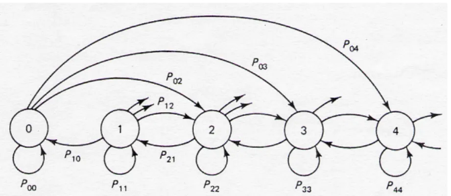
Note that from one state to the next, the state increase by the number of new arrivals transmitted by unbacklogged nodes. Less one, if one new arrival and no backlogged packet, or no new arrival and one backlogged packet is transmitted. Thus the state transition probability, from one state to next is given by
⎪ ⎪ ⎩ ⎪ ⎪ ⎨ ⎧ − = = − + = − ≤ ≤ = + 1 i ), , 1 ( ) , 0 ( 0 i )], , 1 ( 1 )[ , 0 ( ) , 0 ( ) , 1 ( 1 i )], , 0 ( 1 )[ , 1 ( n) -(m i 2 ), , ( , n Q n Q n Q n Q n Q n Q n Q n Q n i Q p r a r a r a r a a i n n (2.3)
Fig. 2.2 Markov chain for slotted Aloha.
Fig. 2.2 illustrates this Markov chain. Note that the state can decrease only 1 in a single transition, but can increase by an arbitrary amount. Then the steady-state probability can be easily calculatedly. Finding pn for each successively larger in terms of p0 , and then finding
as a normalizing constant. From this, the expected number of backlogged node can be found, and from the Little’s theorem, the average delay can be calculated.
Unfortunately, this system has some very strange property for a large number of nodes. Note that choose large retransmission probability moderately large can to avoid large delays after collision. In this situation, small arrival rate and not to many backlogged node, this work well, retransmission are normally successful. But, if backlogged packet get large enough to satisfy qrn>>1, then collisions will occur successively slots for a long time.
To understanding this situation quantitatively, define the driff in state n D as the n
expected change in backlog over one slot time, starting in state n. Thus, D is the expected n
number of new arrivals accepted into the system less the expected number of successful transmissions is just the probability of successful transmission, define as P . Thus . succ
) ( a succ n m n q p D = − − (2.4) where ) , 1 ( ) , 0 ( ) , 0 ( ) , 1 ( n Q n Q n Q n Q psucc = a r + a r (2.5)
Define the attempt rate G(n) as the expected number of attempted transmissions in a slot
when in state n, that is
r a nq q n m n G( )=( − ) +
If q and a qr are small, P is closely approximated as the following function of the succ
attempt rate: ) ( ) ( Gn succ G n e P ≈ − (2.6) This approximation is derived directly from Eq. (2.5), using the approximation (1-x)y ≈ e -
xy for small x in the expressions for Q
a and Qr. similarly, the probability of idle slot is
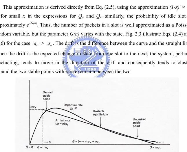
approximately e–G(n). Thus, the number of packets in a slot is well approximated as a Poisson random variable, but the parameter G(n) varies with the state. Fig. 2.3 illustrate Eqs. (2.4) and (2.6) for the case qr > q . The drift is the difference between the curve and the straight line. a
Since the drift is the expected change in state from one slot to the next, the system, perhaps fluctuating, tends to move in the direction of the drift and consequently tends to cluster around the two stable points with rare excursion between the two.
Fig. 2.3 Instability of slotted Aloha. The horizontal axis corresponds to both the state and attempt rate G, which are related by G(n)=(m−n)qa +nqr, with qr>q . a
There are two important conclusions from this figure (Fig. 2.3). First, the departure rate is at most 1/e for large m. Second, the departure rate is almost zero for long periods whenever the system jumps to the undesired stable point. Consider the effect of change qr. As qr is
increased, the delay in retransmitting a collided packet decreases.
If we replace the no-buffering assumption with the infinite-node assumption. The attempt rate G(n) becomes λ+ n qr and the straight line representing arrivals in Fig. 2.3 become horizontal. In this case, the undesirable stable point disappears, and once the system passes the unstable equilibrium, it tends to be without bound. In this case, the corresponding infinite-state Markov chain has no steady state distribution. And the expected backlog increases without bound as the system continuous running.
From a practical standpoint, if the arrival rate λ is very much smaller than 1/e, and if qr
is moderate, then the system could be expected to remain in the desired stable state for a long time. Once unfortunately, move to the undesired stable point, the system could be started with backlogged packets lost.
We look at modification of slotted Aloha that that cure this stability issue. One simple approach to achieving stability is that ( ) G(n)
succ G n e
P ≈ − ,which is maximized at G(n)=1. Thus, it is desirable to change qr dynamically to maintain the attempt rate G(n) at 1. The difficult is that n is unknown to the nodes and only be estimated from the feedback.
With the infinite-node assumption, no arrivals are discarded but the delays become infinite. Therefore, if expected delay per packet is finite, then the system is stable for a given arrival rate. Ordinary slotted Aloha is unstable. Our purpose with this definition is to find a algorithm that do not require knowledge of the number of nodes and maintain small delay. Rivest’s pseudo-Bayesian algorithm is a simple and effective way to stabilize Aloha. Next, we will illustrate this algorithm particularly.
2.2 Pseudo-Bayesian algorithm
Assume that each station has at most one packet to transmit at any time. A station is active if it has a packet to transmit; otherwise, it is inactive. When a slot begins each active station must decide, either deterministically or stochastically, whether or not to transmit its packet.
There are three possible outcomes: (1) a idle if no stations transmit;
(2) a success if one station transmits; or
(3) a collision if more than one station transmits.
This approach has the following general form. Just before slot t begins, each station k in the network computes a value for its broadcast probability bk,t Then station k will transmit a
packet (if it has one) with probability bk,t independent of whether previous attempts had been
made to transmit that packet.
Assume that each station k computes bk,t from the globally available network history,
indicating whether each slot was a hole, a success, or a collision. Since the stations only use global information to compute the broadcast probabilities bk,t, each station will compute the
same value bt for bk,t , and updating procedure will be relatively straightforward.
Let Nt denote the number of active stations at time t. The probabilities of an idle, success,
or collision for a given broadcast probability bt ( and waiting probability wt = 1 - bt ) and
given value Nt = n : n t b t n I n w N idle p t = = = ) ( ) | ( (2.7) 1 ) ( ) | ( = = = ⋅ ⋅ n− t t b t n S n n b w N success p t (2.8) ) ( ) ( 1 ) ( ) | (collision N n C n I n S n p t = = bt = − bt − bt (2.9)
The optimum value for bt is
; / 1 t
t N
This maximizes (Nt)
t
b
S Note that b, depends only on Nt. If bt is chosen optimally as l/
Nt, the expected number of stations attempting to transmit will be one, and the probabilities of
holes, successes, and collisions will be
e N N I t t N t t N 1 1 1 ) ( / 1 ⎟⎟ ≈ ⎠ ⎞ ⎜⎜ ⎝ ⎛ − = (2.11) e N N S t t N t t N 1 1 1 ) ( / 1 ⎟⎟ ≈ ⎠ ⎞ ⎜⎜ ⎝ ⎛ − = (2.12) e N C N t t 2 1 ) ( / 1 ≈ − (2.13)
(The approximations hold for large Nt )
However, the stations will typically not know the correct value for Nt,. For example, some
inactive stations may have received newly generated packets during slot t - 1 which they will be ready to transmit during slot t. In the first procedure we describe, which we call the Bayesian broadcast algorithm, each station will use the evidence available up to time t to estimate the likelihood pn,t that Nt= n for each n≥0. That is,
), Pr(
, N n
pnt = t = for n=0,…… (2.14)
given the available evidence. According to the procedure Bayesian broadcast to estimate ) , , ( 0, 1, ⋅ ⋅⋅ = t t t p p p .
In the Bayesian broadcast procedure, each station begins with the initial distribution
) , 0 , 0 , 1 ( 0 = ⋅ ⋅⋅
p - it assumes that all stations are inactive. Each station will compute the same vector pt using the available global feedback information. The vector
) , , ( 0, 1, ⋅ ⋅⋅ = t t t p p
p summarizes the global information available about Nt.
With the Bayesian broadcast procedure, each station performs the following four steps during each time slot.
(1) Compute the optimal broadcast probability bt, from the initial probability vector pt .
(2) If the station is active, transmit its packet with probability bt.
(3) Perform a Bayesian update of pt (the initial probability distribution for N,) to obtain
'
t
p (the final probability distribution for Nt ), using the evidence (idle, success, or
collision) observed in time slot t.
(4) Convert the final probabilities pt' for Nt, into initial probabilities pt+1 for Nt+1, by
considering the generation of new packets and the fact that a packet may have been successfully transmitted during time slot t.
Derive this algorithm by assuming that pt, can be reasonably approximated by a Poisson distribution with mean nˆ(nˆ is estimated n ) ; Let
! ˆ ) ( ˆ ˆ n n e n P n n n ⋅ = − (2.15)
Denote the Poisson density at n for Poisson parameter ע. Each station will keep only
nˆ,rather than the vectorpt and will approximate the initial probability pn,t by Pnˆ(n).
To develop the pseudo-Bayesian broadcast and probability updating procedure, we first consider the equations that would be used for a true Bayesian update of the
Poisson approximation for pt if bt is the actual broadcast probability (and wt = 1 - bt).
These equations represent the unnormalized final probability values:
) ( ) ( ˆ ) ( ˆ I n e P n P t t t nw b b n n ⋅ = ⋅ − (2.16) ) 1 ( ˆ ) ( ˆ ) ( ˆ ⋅ = ⋅ ⋅ − − P n e b n n S P t t t nw b t b n n (2.17) )) ( ) ( 1 ( ) ( ˆ( ) ) ( ˆ C n P I n S n Pnn ⋅ bt = nn − bt − bt (2.18)
Therefore, it can easily compute broadcast probability:
); 1 , ˆ 1 min( n bt = (2.19)
From (2.16 ) and (2.17), derive decrements nˆ by 1, if the current slot is a hole or a success.
If there is a collision, Bayes’ rule will not yield a Poisson distribution for the final probabilities. However, Rivest approximate the result by a Poisson distribution by setting nˆ
to be the mean of the resulting distribution, which is (using x to denote nˆ⋅bt): 1 ˆ 2 − − + x e x n x (2.20)
which simplifies in the case nˆ≥1,
n bt ˆ 1 = to 2 1 ˆ − + e n (2.21)
The Pseudo-Bayesian Broadcast Procedure: Each station maintains a copy of nˆ and, during each slot. Each backlogged packet is then transmitted ( independently ) with
probability qr = ,1}
ˆ 1 min{
n (note: we replace bt with qr ), the minimum poperation limits qr to at
most 1, and try to achieve an attempt rate G=nqr of 1. For each k, the estimated backlog at the
beginning of slot k+1 is updated from the estimated backlog and feedback for slot k according to the rule
{
}
⎩ ⎨ ⎧ − + + − + = − + ˆ ( 2) , for collision success or idle for , 1 ˆ , max ˆ 1 1 e n n n k k k λ λ λ (2.22) The maximum operation ensures that the estimate is never less than the contribution from new arrivals. On successful transmission, subtracting 1 from the previous backlog. And subtracting 1 from the previous backlog on idle slot, has the effect to avoid that too many idle occur. Finally, adding (e-2)-1 on collision has the effect to decreasing nˆ when too many collision occur. Thus G(n) is 1,and, by the Poisson approximation , idle occurs with probability 1/e and collisions with probability (e-2)/e, so that decreasing nˆ by 1 on idles and increasing nˆ by (e-2)-1 on collisions maintains the balance between n and nˆ on average. On successful or idle transmission, nˆk+1=max{
λ,nˆk +λ−1}
, and On collision, updating with 11 ˆ ( 2)
ˆ −
+ =n + + e−
nk k λ .
In applications, the arrival rate λ is typically unknown and slowly varying. Thus, the algorithm must ether estimate λ from time-average rate of successful transmissions or set it’s value within the algorithm to some fixed value. It has been shown by Milkhailov and Tsitsiklis that if the fixed value 1/e us used within the algorithm, stability is achieved for all actual λ <1/e. nothing has been proven about the behavior of the algorithm when a dynamic estimate of λ is used within the algorithm.
Note that since each station now only maintains a single parameter nˆ, it would be simple to broadcast nˆ with every packet. In this way stations which have just powered-up can
“synchronize” easily.
2.3 Splitting Tree Algorithms
The slotted Aloha requires some care for stabilization and is also essentially limited to throughputs of 1/e. We now want to look at more sophisticated collision resolution techniques that both maintain stability and also increase the achievable throughput. A splitting algorithm is an approach that divides the users involved in a collision into several subsets. Only the user or users in one of the subsets will transmit at the next time slot so that the probability of collision is reduced.
The first splitting algorithms were algorithms with a tree structure. When a collision occurs, say in the kth slot, all nodes not involved in the collision go into a waiting mode, and all those involved in the collision split into two subsets (e.g., by each flipping a coin). The first subset transmits in slot k+1, and if that slot is idle or successful, the second subset transmits in slot k+2 (see Fig. 2.2). Alternatively, if another collision occurs in slot
k+1, the first of these two subsets split again, and the second subset waits for the resolution
of that collision.
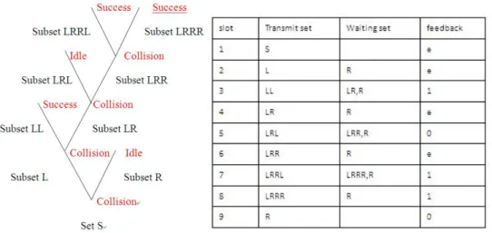
The rooted binary tree in Fig. 2.4 represents a particular pattern of idles, success, and collision resulting from such a sequence of splitting. S represents the set of packets in the original collision, and L (left) and R (right) represent the two subsets that S splits into. Similarly, LL and LR represent the two subsets that L splits into after L generates a collision. The set of packets corresponding to the root vertex S is transmitted first, and after the transmission of the subset corresponding to any nonleaf vertex, the subset corresponding to the vertex on the left branch, and all of its descendant subsets, are transmitted before the subset of the right branch. Given the immediate feedback we have assumed, it should be clear that each node, in principle, can construct this tree as the 0, 1, e feedback occurs; each node can keep track of its own subset in the tree, and thus each node can transmits its own backlogged packet.
The transmission order above corresponds to that of a stack. When a collision occurs, the subset involved in collision is split, and each resulting stack is pushed on the stack (i.e., each stack element is a subset of nodes); then the head of the stack (i.e., most recent subset pushed on the stack) is removed from the stack and transmitted. The list, from left to right, of waiting subsets in Fig. 2.4 corresponds to the stack elements starting at the head for the given slot. Note that a node with backlogged packet can keep track of when to transmit by a counter determining the position of the packet’s current subset on the stack. When the packet is involve in a collision, the counter is set to 0 or 1, corresponding to which subset the packet is placed in. When the counter is 0, the packet is transmitted, and if the counter is nonzero, it is incremented by 1 for each collision and decremented by 1 for each success or idle.
One problem with this tree algorithm is what to do with the new packet arrivals that come in while a collision is being resolved. A collision resolution period (CRP) is
defined to be completed when a success or idle occurs and there are no remaining elements on the stack (i.e., at the end of slot 9 in Fig. 2.4). At this time, a new CRP starts using the packets that arrived during the previous CRP. In the unlikely event that a great many slots are required in the previous CRP, there will be many new waiting arrivals, and these will collide and continue to collide until the subsets get small enough in the new CRP. The solution to this problem is as follow: At the end of a CRP, the set of nodes with new arrivals is immediately split into j subsets, where j is chosen so that the expected number of packets per subset is slightly greater than 1 (slightly greater because of the temporary high throughput available after a collision). These new subsets are then placed on the stack and the new CRP starts.
Chapter 3
A Pseudo-Bayesian-Broadcast-Based MAC
Protocol
In this chapter we will introduce our “A Pseudo-Bayesian-Broadcast-Based MAC Protocol algorithm”. Because the number of nodes, n, is unknown. Each node should maintain the estimate nˆ to decide the transmission probability.
3.1 Model
We list the assumptions of the model and then discuss their implications.
1. Slotted system. Assume that all transmitted packet have the same length and that
each packet requires one time unit (call a slot) for transmission. All transmitters are synchronized so that the reception of each packet starts at an integer time and ends before the next integer time.
2. Poisson arrivals. Assume that packets arrival for transmission at each of the m
transmitting nodes according to independent Poisson process. Let λ be the overall arrival rate to the system,
3. Noisy collision channel. Assume that if two or more nodes send a packet in a
given time slot, then there is a collision and receiver obtain no information about the contents or source of the transmitted packet. But packets can be corrupted also by noise
even when collisions are absent.
4. 0,1,e Immediate feedback. At the end of each slot, each node detects whether 0
packet, 1 packet or more than one packet were transmitted in that slot.
5. Retransmission of collisions. Assume that each packet involved in a collision must
be retransmitted in some later slot, with further such retransmission until the packet is successfully received. A node with a packet that must be retransmitted is said to be backlogged.
6. A .No buffering. If one packet at a node is currently waiting for transmission or
colliding with another packet during the transmission, new arrivals at that node are discarded and never transmitted. An alternative to this assumption is the following.
B. Infinite set of nodes (m=∞). The system has an infinite set of nodes and each
newly arriving packet arrives at a new node.
3.2 A Pseudo-Bayesian-Broadcast-Based MAC Protocol
In the “A Pseudo-Bayesian-Broadcast-Based MAC Protocol”, we have some differences with the “tree splitting algorithm”.
1. In the CRP start each node transmits with probability 1/nˆ.The estimate nˆ is maintain by each node, and using Pseudo-Bayesian and “A Pseudo-Bayesian-Broadcast-Based MAC Protocol to update” estimate nˆ. And how to update estimate nˆ, we will illustrate detail in next segment. We might transmit
successfully in one slot with probability 1/e, when N is large enough.
2. We judge that a CRP is end when the five cases occur. And there are two kind of CRP time period, one period is spending 1 slot time, and the other is 3 slot time.
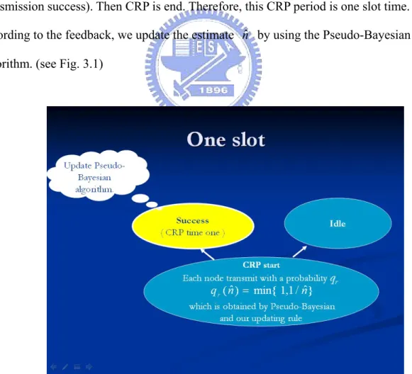
2.1 The “Success” occurs : When last CRP is end, and new CRP is start. At CRP time one, each node transmit packet with probability qr(nˆ)= ,1}
ˆ 1 min{
n .At the beginning of the CRP, nodes which transmit packet
split to the left subset L, and nodes which do not transmit packet split to the right subset R. At the end of CRP time one, if receiving feedback is 1 (mean that CRP time one
transmission success). Then CRP is end. Therefore, this CRP period is one slot time. And according to the feedback, we update the estimate nˆ by using the Pseudo-Bayesian algorithm. (see Fig. 3.1)
Fig. 3.1 CRP time one transmission success. CRP time period is 1.
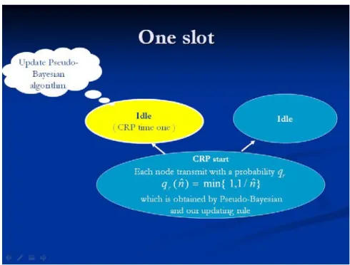
When last CRP is end, and new CRP is start. At CRP time one, each node transmit packet with probability qr(nˆ)= ,1}
ˆ 1 min{
n .At the beginning of the CRP, nodes which transmit
packet split to the left subset L, and nodes which do not transmit packet split to the right subset R. At the end of CRP time one, if receiving feedback is 0 (mean that CRP time one, no one transmits packet). Then CRP is end. Therefore, this CRP period is one slot time. And according to the feedback, we update the estimate nˆ by using the Pseudo-Bayesian algorithm. (see Fig. 3.2)
Fig. 3.2 CRP time one transmission feedback is idle. CRP time period is 1.
2.3 The “Collision” occurs :
2.3.1 case one: CRP time two “Idle”
When last CRP is end, and new CRP is start. At CRP time one, each node transmit packet with probability qr(nˆ)= ,1}
ˆ 1 min{
n .At the beginning of the CRP, nodes which transmit
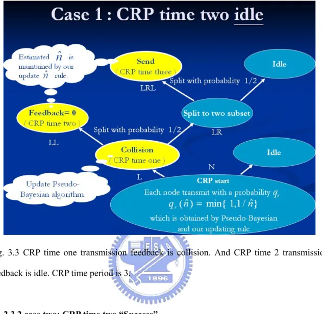
packet split to the left subset L, and nodes which do not transmit packet split to the right subset R. At the end of CRP time one, if receiving feedback is e (mean that CRP time one,
more than two node transmit packet and occur collision). And according to the feedback, we update the estimate nˆ by using the Pseudo-Bayesian algorithm.
Then next slot enter CRP time two. The nodes in the subset L now splitting to two subset LL and LR with probability 1/2, and nodes which splitting to the subset LL transmit packet immediately. Such that if more than 2 nodes in subset LL will occur collision. Only if one node is in subset LL, then the feedback is 1. Otherwise, no one is in subset LL, then the feedback is 0 (idle). If at the end of time two, the receive feedback is 0 (mean that CRP time two, no one transmits packet). According to this feedback, we update the estimate nˆ
by our updating algorithm (we will illustrate detail in next segment).
Then enter the CRP time three. Usually, the tree-splitting algorithm, will let nodes in subset LR transmit packet. But because time 2 feedback is 0, such that subset LR have more than 2 node ready to transmit. If we transmit node in subset LR, must occur collision. So, we let nodes which are in subset LR splitting again with probability 1/2. Then node which is splitted to subset LRL, can transmit packet. And we use the feedback to update the estimate
nˆ by calculating our updating algorithm. Then CRP is end. CRP period is three slot time. (see Fig. 3.3)
Fig. 3.3 CRP time one transmission feedback is collision. And CRP time 2 transmission feedback is idle. CRP time period is 3.
2.3.2 case two: CRP time two “Success”
When last CRP is end, and new CRP is start. At CRP time one, each node transmit packet with probability qr(nˆ)= ,1}
ˆ 1 min{
n .At the beginning of the CRP, nodes which transmit
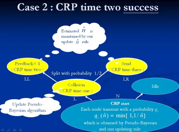
packet split to the left subset L, and nodes which do not transmit packet split to the right subset R. At the end of CRP time one, if receiving feedback is e (mean that CRP time one, more than two node transmit packet and occur collision). And according to the feedback, we update the estimate nˆ by using the Pseudo-Bayesian algorithm.
Then next slot enter CRP time two. The nodes in the subset L now splitting to two subset LL and LR with probability 1/2, and nodes which splitting to the subset LL transmit
packet immediately. If at the end of time two, the receive feedback is 1 (mean that CRP time two, only one transmits packet). According to this feedback, we update the estimate nˆ by our updating algorithm (we will illustrate detail in next segment).
Then next slot enter the CRP time three. And let nodes in subset LR transmit packet immediately. At the end of CRP time 3, we use the feedback to update the estimate nˆ by calculating our updating algorithm. Then CRP is end. And this CRP period is three slot time. (see Fig. 3.4)
Fig. 3.4 CRP time one transmission feedback is collision. And CRP time 2 transmission feedback is success (1). CRP time period is 3.
2.3.1 case three: CRP time two “collision”
When last CRP is end, and new CRP is start. At CRP time one, each node transmit packet with probability qr(nˆ)= ,1}
ˆ 1 min{
n .At the beginning of the CRP, nodes which transmit
packet split to the left subset L, and nodes which do not transmit packet split to the right subset R. At the end of CRP time one, if receiving feedback is e (collision). And according to the feedback, we update the estimate nˆ by using the Pseudo-Bayesian algorithm.
Then next slot enter CRP time two. The nodes in the subset L now splitting to two subset LL and LR with probability 1/2, and nodes which splitting to the subset LL transmit packet immediately. If at the end of time two, the receive feedback is e (mean that CRP time two collision, and more than one node transmits packet). According to this feedback, we update the estimate nˆ by our updating algorithm (we will illustrate detail in next segment).
Then enter the CRP time three. Because time 2 feedback is e, such that subset LL will split again with probability 1/2. Then node which is splitted to subset LLL, can transmit packet. And at the end of CRP time 3, we use the feedback to update the estimate nˆ by calculating our updating algorithm. Then CRP is end, and CRP period is three slot time. (see Fig. 3.5)
Fig. 3.5 CRP time one transmission feedback is collision. And CRP time 2 transmission feedback is collision (e). CRP time period is 3.
3.3 Estimate
nˆ
algorithm
There are two algorithms to maintain estimate nˆ in our research. One is Pseudo-Bayesian algorithm, and it will be use to calculate nˆ at the end of CRP time one. The other is our estimate nˆ algorithm, it will be apply at the end of CRP time two and time three.
Pseudo-Bayesian algorithm is introduced in background knowledge. And this segment, we will introduce our estimate nˆ algorithm.
For each k, the estimated backlog at the beginning of slot k+1 is updated from the estimated backlog and feedback for slot k according to the rule
{
}
⎩ ⎨ ⎧ + + =+ ˆ 0.423, for idleandcollision
success for , 1 - 423 . 0 ˆ , 3 42 . 0 max ˆ 1 k k k n n n (3.1)
The maximum operation ensures that the estimate is never less than the contribution from new arrivals. On successful transmission, subtracting 1 from the previous backlog. The algorithm must ether estimate λ from time-average rate of successful transmissions or set it’s value within the algorithm to some fixed value. It has been shown by Milkhailov and Tsitsiklis that if the fixed value used within the algorithm, stability is achieved for all actual λ < maximum throughput. Therefore we choose 0.43 as the fixed value, stability is achieved for all actual λ < 0.423 (maximum throughput will be prove at next chapter). For idle and collision, because no one leave the system, therefore adding a estimate λ.
In CRP, increase the estimated n at the maximum expected rate in stabilized region. Therefore, the only chance with positive probability is that estimated n is larger than real n. In the case of larger estimated n, it enters in the second mode with less chance. Besides, the probability of idle becomes larger and thus estimated n will be decreased around real n with larger probability.
Chapter 4
Throughput analysis
In this section, we will analyze the average throughput.
The average throughput is equal to the total successful number divided by the total time slots. CRP] a in slots time E[ CRP] a in numbers successful E[ CRP] a in ut E[throughp Throughput Average = = (4.1)
To calculate the equation we need to calculate attributes first.
Sk: the expected value of successful nodes in a CRP given the condition that k nodes split to the left subset when a CRP starts.
Pk: the probability that k nodes split to the left subset when a CRP starts.
! 1 ) 1 ( ) 1 ( lim e k N N N C P N k N k k N k ≅ ⋅ − = − ∞ → (4.2)
So the equation (4.1) may be restated as
] CRP a in slots time [ E S P Throughput k k k
∑
=There are two kind of CRP length:
(1).At the beginning of CRP starting, if feedback is 0 or 1. Then CRP need one slot time. (2).Otherwise, at the beginning of CRP starting, if feedback is e, then CRP need 3 slot time.
528482235 . 1 3 2 1 1 1 1 1 ] CRP a in slot E[ = × ⎟ ⎠ ⎞ ⎜ ⎝ ⎛ − + × ⎟ ⎠ ⎞ ⎜ ⎝ ⎛ + × ⎟ ⎠ ⎞ ⎜ ⎝ ⎛ = e e e (4.3)
E[success numbers in a CRP ] can be generalize as four type to calculate the value.
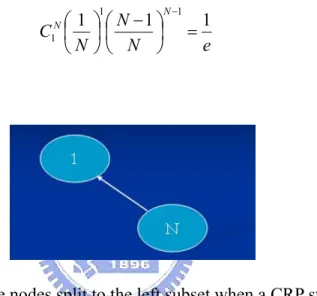
Case one:
Assume that there is one node splitting in the left subset (Fig. 4.1). Then the probability of transmission success is that:
e N N N C N N 1 1 1 1 1 1 ⎟ = ⎠ ⎞ ⎜ ⎝ ⎛ − ⎟ ⎠ ⎞ ⎜ ⎝ ⎛ − (4.4)
Fig. 4.1 one nodes split to the left subset when a CRP starts
Case two:
We assume that there are k nodes (k≥2) splitting in the left subset, and CRP time 2 feedback is 0 (Fig. 4.2), then the probability of one node transmission success is that:
(
)
2 ,K 2,3,4,....,N 1 ! 1 1 2 1 2 1 1 1 2 1 0 = ⎟ ⎠ ⎞ ⎜ ⎝ ⎛ ⋅ − ≈ ⎟ ⎠ ⎞ ⎜ ⎝ ⎛ × ⎟ ⎠ ⎞ ⎜ ⎝ ⎛ × ⎟ ⎠ ⎞ ⎜ ⎝ ⎛ − ⎟ ⎠ ⎞ ⎜ ⎝ ⎛ − K K K K K K N K N K e K C C N N N C (4.5)Fig. 4.2 k≥2 nodes split to the left subset when a CRP starts and CRP time 2 feedback is 0.
Case three:
We assume that there are k nodes (k≥2) splitting in the left subset, and CRP time 2 feedback is 1 (Fig. 4.3), then the probability of one node transmission success is that:
(
)
2 K 2,3,4,...,,N 1 ! 1 1 2 1 1 1 1 ⎟ = ⎠ ⎞ ⎜ ⎝ ⎛ − ≈ ⎟ ⎠ ⎞ ⎜ ⎝ ⎛ × ⎟ ⎠ ⎞ ⎜ ⎝ ⎛ − ⎟ ⎠ ⎞ ⎜ ⎝ ⎛ − K K K K N K N K e K C N N N C (4.6)Fig. 4.3 k≥2 nodes split to the left subset when a CRP starts and CRP time 2 feedback is 1.
Case four:
We assume that there are k nodes (k≥2) splitting in the left subset L, and CRP time 2, there are j nodes (2≤j≤k) splitting in the left subset LL (feedback is e ), then the probability of one node transmission success is that: (Fig. 4.4)
K , 2,3,4,.... J and N 2,3,4..., K 2 1 )! 1 ( )! ( 1 2 1 2 1 1 1 J K 1 = = ⎟ ⎠ ⎞ ⎜ ⎝ ⎛ − − ≅ ⎟ ⎠ ⎞ ⎜ ⎝ ⎛ × ⎟ ⎠ ⎞ ⎜ ⎝ ⎛ × ⎟ ⎠ ⎞ ⎜ ⎝ ⎛ − ⎟ ⎠ ⎞ ⎜ ⎝ ⎛ + − e J J K C C N N N C J J K K J K N K N K (4.7)
Fig. 4.4 k≥2 nodes split to the left subset when a CRP starts and CRP time 2 feedback is e.
E[success numbers in a CRP ]=
∑
≥ + + + 2 k four case three case two case one case => 0.423 ] CRP a in slots time [ ] CRP a in numbers E[success ≅ = E ThroughputChapter 5
Simulator and simulation results
In this section we will introduce our simulator briefly and then present our simulation results.
5.1 Simulator
We use UML (Unified Machine Language) to simulate the environment. The OMD (Object Main Diagram) is as illustrated in Fig. 5.1 below. When the simulation starts, one object of “nodegenerator” generates objects of “standbysystem”, of “node”, of “channel”, and sets all links. The object of “nodegenerator” generates nodes by Poison random arrival (State Chart of nodegenerator is Fig. 5.2 below). The object of “node” transmit packet with probability qr(nˆ)= ,1}
ˆ 1 min{
n . And according to different CRP status, do corresponding
action. The object of “channel” indicates the channel condition, all nodes listen the channel feedback (State Chart of channel is Fig. 5.3 below).
Fig. 5.1 OMD of the Simulator.
Fig. 5.2 State Chart of “nodegenerator”.
5.2 Simulation results
To evaluate the performance of “A Pseudo-Bayesian-Broadcast-Based MAC Protocol”, two performance metrics are discussed: system throughput and the average delay of system. The throughput is defined as the number of success packets transmitted in one slot. The average delay is defined as the time from the packet generation to the packet transmitting successfully.
For run 106 time slots, and estimate λ of Pseudo-Bayesian and our algorithm is 0.423. Fig.5.10 when arrival rate is 0.43, the system become unstable.
And from Fig.5.4~Fig5.12, We can see if arrival rate much smaller than throughput 0.43, the backlog n is similar the estimate nˆ, and the average backlog is much smaller.
Backlog and estimate backlog vs. time.
Fig. 5.6 arrival rate=0.3 Fig. 5.7 arrival rate=0.4
Fig. 5.8 arrival rate=0.41 Fig. 5.9 arrival rate=0.42
Fig. 5.10 arrival rate=0.43 Fig. 5.11 arrival rate=0.99
From Fig. 5.12 when arrival rate small than 0.43, the average delay is small, otherwise increasing rapidly. From Fig.5.13 when arrival rate < 0.43, the throughput is equal to arrival rate. In Fig.511, the result shows that if arrival rate less than 0.43, the average delay is small. If arrival rate is approach to 1, the delay increasing slowly, because although delay increasing but success transmission decreasing, this delay could not be calculated. In Fig.5.15, we can see the throughput larger slightly than we calculate in previous chapter. It is because nˆ is smaller than n, therefore transmission probability increasing, although success transmission
decreasing, but it decreases slowly, and two node occur collision raising, but using our splitting policy, can effectively result two node collision.
Fig. 5.12 average delay time vs. arrival rate
ARRIVAL RATE AVERAGE DELAY THROUGHPUT 0.1 0.373199 0.100453 0.15 0.657040 0.149691 0.2 1.106567 0.200194 0.25 1.873979 0.250013 0.3 3.354199 0.300388 0.35 7.174506 0.350682 0.4 28.845044 0.401017 0.41 55.942554 0.410819 0.42 116.321966 0.420022 0.43 6557.502004 0.424208
Table 5.1 the average delay and throughput for each arrival rate, and simulation 106 time slot.
Fig. 5.15 throughput vs. arrival rate (0.1~0.99)
ARRIVAL RATE AVERAGE DELAY THROUGHPUT
0.1 0.388252 0.100270 0.2 1.155163 0.200950 0.3 3.625937 0.302730 0.4 24.491672 0.403440 0.41 51.135637 0.412720 0.42 169.327422 0.421780 0.43 719.881853 0.423710 0.45 2829.174162 0.424950 0.5 6631.537807 0.425710 0.6 11635.073822 0.414510 0.7 14692.510595 0.406800 0.8 16151.262192 0.381820 0.9 18167.687137 0.370290 0.99 19113.857283 0.356230 Table 5.2 The average delay and throughput for each arrival rate, and simulation 105 time slot.
Chapter 6
Conclusion
As in Rivest’s Pseudo-Bayesian algorithm, our purpose is to find an algorithm that does not require the acknowledgement of the number of nodes, and increase the throughput. In our thesis, for the second mode we also consider a splitting algorithm. However, our version of splitting algorithm does not include the common receiver and thus doing so renders it more applicable to wireless access system. Using our method is to estimate nˆ of the backlog n by receiving the feedback and to combine our splitting algorithm police to reduce collision. Finally, the throughput by using our policy is 0.423. And when arrival rate < 0.423, we can see that estimate nˆ is similar to n and average delay time is small.
Reference
[1] D.Bertseks et al., Data networks, Englewood Cliffs, NJ: prentice-Hall, 1992.
[2] R. Rivest, “Network control by bayesian broadcast.” IEEE Transactions on Information Theory, Vol 33, pp.323-328, May 1987.
[3] E. Altman, R. El-Azouzi, T. Jim´enez, “Slotted Aloha as a stochastic game with partial information”, Computer Networks, 2004.
[4] F. Cali, M. Conti and E. Gregori, "IEEE 802.11 Wireless LAN: Capacity Analysis and Protocol Enhancement," in Proceedings of INFOCOM'98, Mar. 1998.
[5] Chih-Yung Shih, Ray-Guang Cheng, Chung-Ju Chang, “Achieving Weighted Fairness for Wireless Multimedia Service”, Vehicular Technology Conference, 2003. VTC 2003-Fall. 2003 IEEE 58th Volume 4, 6-9 Oct. 2003 Page(s):2381 - 2385 Vol.4 .
[6] Alberto Leon-Garcia and Indra Widjaja, “Communication Networks: fundamental concepts and key architecture” 2nd Ed.
[7] A.B. MacKenzie, S.B. Wicker, "Stability of Multipacket Slotted Aloha with Selfish Users and Perfect Information", Proc. of IEEE INFOCOM 2003, 2003, Vol. 3, pp. 1583-1590.