油價及國內生產毛額對高速公路交通量之影響

國 立 交 通 大 學

管理學院碩士在職專班

運輸物流組

碩士論文

An Empirical Investigation into the Effects of Gas

Price and GDP on Freeway Traffic

研 究 生：楊淑津

指導教授：邱裕鈞 博士

油價及國內生產毛額對高速公路交通量之影響

An Empirical Investigation into the Effects of Gas Price and GDP on

Freeway Traffic

研 究 生：楊淑津 Student: Shu-Chin Yang

指導教授：邱裕鈞博士 Advisor: Dr.

Yu-Chiun Chiou

國 立 交 通 大 學

管理學院碩士在職專班運輸物流組

碩 士 論 文

A Thesis

Submitted to Degree Program of Transportation and Logistics College of Management

National Chiao Tung University in Partial Fulfillment of the Requirements

for the Degree of Master of Science

in

Transportation and Logistics

June 2010

Taipei, Taiwan, Republic of China

油價及國內生產毛額對高速公路交通量之影響

學生：楊淑津 指導教授：邱裕鈞 博士

國 立 交 通 大 學

管理學院碩士在職專班運輸物流組

碩 士 論 文

摘要

摘要

摘要

摘要

本研究旨在探討民國九十三年一月至九十八年六月間油價及國內生產毛額對高 速公路各收費站通行車輛數之長短期因果關係及跨期動態之衝擊反應，俾提供有關 單位交通量管理策略研擬之參考。本研究首先將各收費站通行車輛數通行車輛的月 資料依路線（國道 1 號、3 號、5 號）、區域（北區、中區、南區、宜蘭地區、全 島）及車種（小型車、大型車、聯結車）加以區隔分析。在實證方法上的選用是 以 Engle and Granger 兩 階 段 法 及 Johansen 最 大 概 似 法 進 行 共 整 合 檢 定 （cointegration test），來檢定變數間是否存在長期均衡關係。並根據 Granger(1969) 所提出變數預測力的方法, 利用 Wald 檢定及 Toda and Yamamoto (1995)之方法來 衡量變數間之短期領先落後的因果關係。最後，再輔以向量自我迴歸模型進行後續 的衝擊反應函數分析，以了解變數間之動態、跨期的影響與衝擊，俾檢視我國油 價、國內生產毛額及高速公路交通量間是否存在緊密的關係。

實證結果發現，兩種共整合之檢定結果皆顯示油價及國內生產毛額與高速公路 交通量不存在長期均衡共整合的關係。此說明了長期的交通量之增減並無法由油價 及國內生產毛額來加以判定，而係由其他因素所左右。此外，不同 Granger 因果關 係的檢定方法雖產生部份結果不一致之現象，但就宜蘭地區而言，兩種 Granger 因 果檢定的結果均一致指出該地區之高速公路交通量並不受油價及國內生產毛額的影 響。這顯示國道 5 號交通量仍受其他因素所控制，此與該條國道大部分均為旅遊觀 光旅次與雪山隧道的該開通未台灣北部及東北部的交通帶來很大的便利性有關。最 後，透過衝擊反應函數進行變數間之動態跨期衝擊影響分析中，發現油價及國內生 產毛額對部分地區大型車及聯結車有正向且立即的短暫性衝擊。這說明若有關單位 欲透過油價調整來長期且有效抑制高速公路交通量恐難達成。 關鍵字 關鍵字 關鍵字 關鍵字： 共整合、Granger 因果關係、衝擊反應函數。

An Empirical Investigation into the Effects of Gas Price and GDP on

Freeway Traffic

Student: Shu-Chin Yang

Advisor: Dr. Yu-Chiun Chiou

Degree Program of Transportation and Logistics

College of Management

National Chiao Tung University

Abstract

It is a concept universally acknowledged that when gas price rises, the toll road use will reduce. It is also well-fixed in the minds of many policy makers that they devise energy-related policies based on this premise. With an aim to successfully implement the government’s proposed green tax policy for achieving certain levels of environmental protection by increasing the gas price to reduce the usage of vehicles, the causal effect of gas price and traffic volume plays a significant role here. As a result, this study takes a closer look at the conceptual grounds of the notion of causality in Granger’s sense. In addition, taking into account that GDP may be also a key component of affecting vehicle usage, it is also incorporated into the study.

Cointegration test for the long term equilibrium relationship, Granger causality test for the short run lead or lag relationship and the analysis of impulse response function are employed to unveil and justify the linkage among the interested variables. The main findings are not in line with what we used to take for granted that no co-integration for the long run, not all the gas price or GDP Granger cause traffic volume and as well as some positive impulse responses of traffic volume to gas price shock and GDP innovation. However, as even the simplest descriptive statistics can be deceptive, our findings must be treated with caution especially when extrapolating any anticipated effects on relative policy making.

Keywords: Gas Price, GDP, Freeway Traffic, Cointegration, Granger Causality, Impulse Response Function.

Acknowledgements

In this study, I think I am in the same boat same as the other great thinkers of our times - Plato, Aristotle and Galileo among others, bewildered and unable to unveil the real causality between the economic variables in real world. However, there is one thing for sure that there is a cause-and-effect relationship between the assistance I have received from people around me and the finishing process of this thesis over this period of time at National Chiao Tung University. I am indebted to the following persons.

First of all, I would like to express my deepest appreciation to my advisor - Prof. Yu-Chiun Chiou. Thank you for your advice and spending your valuable time with me. There were more than two hundreds of emails exchanges between us regarding my thesis for the past year. You have shed light on my questions and guided me back on the track when I got lost in time series methodologies. Without your guiding hands, this thesis would be like a star out of reach.

And a big thank you to Prof. Jinn-Tsai Wong, Prof. Cherng-Chwan Hwang, Prof. Tai-Sheng Huang, and Prof. Jiuh-Biing Sheu for your encouragement and enlightenment during the thesis discussion class as well as your comments on my writing. Your advices serve as a magnifier highlighting my problem areas in my study, making it possible for me to revise and improve my thesis.

Thanks a lot to the committee members – Prof. Jin-Li Hu and Prof. Rong-Chan Jou for giving such a meticulous reading to my thesis, and offering many constructive suggestions regarding my thesis writing during the oral defense.

Pooh, no other words can express my feelings better toward your big help in every aspect except what you ever quoted for me from George Eliot, “What greater thing is there for two human souls, than to feel that they are joined for life, - to strengthen each other in all labour, to rest on each other in all sorrow, to minister to each other in all pain, to be one with each other in silent unspeakable memories? “ Thank you. Thank you for everything.

Finally, Jackie, even though your trying to distract me unwittingly nearly made my study impossible, still, thank you for your understandings and moral support all the time especially when there were clouds in my way to the road I less travelled by in my academic journey. They mean a lot to me. I owe you so much.

With all of your assistance and support during the thesis writing process, I am able to lift my spirit, muster my courage and maintain my passion to sail through the rite of the academic passage at NCTU. Thank you everyone for coming into my aid to enrich my life in your own way. Parting is such a sweet sorrow. When I have to farewell my love – NCTU, similar to Earnest Hemmingway who once described his experience in Paris as his moveable feast, luckily, I’ve also had my share of moveable feast right here at NCTU. If you happen to pass it, kiss it for me.

TABLE OF CONTENTS

中文摘要 中文摘要 中文摘要 中文摘要……….………….i ABSTRACT………..…………iii ACKNOWLEDGEMENTS………..…………iv TABLE OF CONTENTS……….v LIST OF TABLES………...…..vi LIST OF FIGURES……….vii CHAPTER 1 INTROCUTION... 1

1.1 BACKGROUND AND MOTIVATION ... 1

1.2 RESEARCH OBJECTIVE ... 5

1.3 RESEARCH SCOPE ... 6

1.4 RESEARCH PROCEDURE ... 8

CHAPTER 2 LITERATURE REVIEW ... 10

2.1 FACTORS AFFECTING DRIVING CHOICE BEHAVIOR ... 11

2.2 IMPACT OF GAS PRICE SHOCKS ON TRAFFIC... 12

2.3 IMPACT OF GDP PRICE INNOVATION ON TRAFFIC... 14

CHPATER 3 METHODOLOGY ... 17

3.1 UNIT ROOT... 17

3.2 CHOOSING THE LAG LENGTH FOR THE UNIT ROOT TEST ... 22

3.3 COINTEGRATION... 23

3.4 VECTOR AUTOREGRESSION MODEL (VAR) ... 28

3.5 GRANGER CAUSALITY... 29

3.6 IMPULSE REPONSE FUNCTION ... 34

CHPATER 4 DATA COLLECTION AND ANALYSIS... 36

4.1 THE DATA... 36

4.2 DESCRIPTIVE STATISTICS... 40

CHPATER 5 EMPIRICAL RESUTLS ... 52

5.1 UNIT ROOT TESTS ... 53

5.2 COINTEGRATION TESTS ... 57

5.3 GRANGER CAUSALITY TESTS ... 61

5.4 IMPULSE RESPONSE ANALYSIS ... 67

CHPATER 6 CONCLUSIONS AND SUGGESTIONS ... 76

6.1 CONCLUSIONS ... 76

6.2 SUGGESTIONS ... 80

REFERENCE ... 81

LIST OF TABLES

TABLE 4.1 VARIABLE DENOTATION AND DEFINITION……….….…37

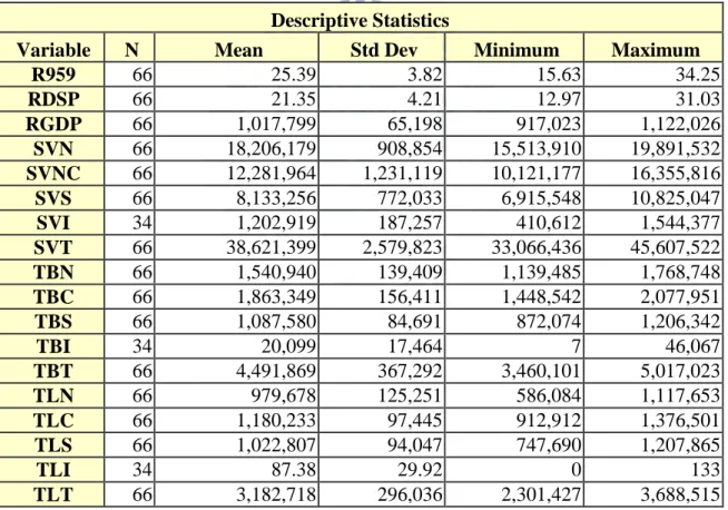
TABLE 4.2 DESCRIPTIVE STATISTICS…….……….….40

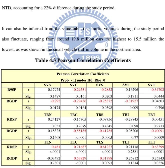
TABLE 4.3 PEARSON CORRELATION COEFFICIENTS…….………41

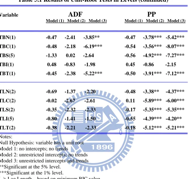
TABLE 5.1 RESULTS OF UNIT-ROOT TESTS IN LEVELS……….53

TABLE 5.2 RESULTS OF UNIT-ROOT TESTS IN FIRST DIFFERENCE……..56

TABLE 5.3 RESULTS OF COINTEGRATION BY THE ENGLE-GRANGERTWO-STEP METHOD……….………58

TABLE 5.4 RESULTS OF COINTEGRATION BY JOHANSEN COINTEGRATION TEST FOR RDSP & TBI...59

TABLE 5.5 RESULTS OF COINTEGRATION BY JOHANSEN COINTEGRATION TEST FOR RGDP & TBI…………...………60

TABLE 5.6 RESULTS OF GRANGER CAUSALITY TESTS……….……….62

LIST OF FIGURES

FIGURE 1.1 SCOPE OF THE STUDY……….…..6 FIGURE 1.2 MAP OF NATIONAL FREEWAY NO. 1, 3 AND 5……….….………..7 FIGURE 1.3 THE STUDY OF RELATIONSHIP BETWEEN VARIABLES IN

THIS RESEARCH………..……….7 FIGURE 1.4 RESEARCH FLOW……….…….……….9 FIGURE 4.1 MONTHLY NATIONAL FREEWAY SMALL VEHICLE TOLL

TRAFFIC VS. REAL 95 LEADFREE GAS PRICE……….….44 FIGURE 4.2 MONTHLY NATIONAL FREEWAY SMALL VEHICLE TOLL

TRAFFIC VS. REAL GDP……….…..45 FIGURE 4.3 MONTHLY NATIONAL FREEWAY TRUCK AND BUS TOLL

TRAFFIC VS. REAL DIESEL PRICE……….………..47 FIGURE 4.4 MONTHLY NATIONAL FREEWAY TRUCK AND BUS TOLL

TRAFFIC VS. REAL GDP……….……….…….48 FIGURE 4.5 MONTHLY NATIONAL FREEWAY TRAILER TOLL TRAFFIC

VS. REAL DIESEL PRICE………..…50 FIGURE 4.6 MONTHLY NATIONAL FREEWAY TRAILER TOLL TRAFFIC

VS. REAL GDP……….……….………51 FIGURE 5.1 ANALYTICAL PROCEDURE FOR TESTING GRANGER

CAUSALITY……….…….52 FIGURE 5.2 PLOTS OF SMALL VEHICLE TOLL TRAFFIC IMPULSE

RESPONSE TO 95 LEAD-FREE GAS PRICE………….……….……70 FIGURE 5.3 PLOTS OF TRUCK AND BUS TOLL TRAFFIC IMPULSE

RESPONSE TO PREMIUM DIESEL GAS PRICE………..71 FIGURE 5.4 PLOTS OF TOLL TRAFFIC IMPULSE RESPONSE TO PREMIUM

DIESEL GAS PRICE………72 FIGURE 5.5 PLOTS OF SMALL VEHICLE TOLL TRAFFIC IMPULSE

FIGURE 5.6 PLOTS OF TRUCK AND BUS TOLL TRAFFIC IMPULSE

RESPONSE TO GDP……….………..74 FIGURE 5.7 PLOTS OF TRAILER TOLL TRAFFIC IMPULSE RESPONSE TO

GDP……….……….….……….75 FIGURE 7.1 PLOTS OF TREND AND CORRELATION ANALYSIS FOR

SERIES IN LEVELS…..…………..………87 FIGURE 7.2 PLOTS OF TREND AND CORRELATION ANALYSIS FOR

To drive or not to drive, that is a question during the rising

gasoline price era.

CHAPTER 1 INTROCUTION

1.1 BACKGROUND AND MOTIVATION

Gasoline price fluctuates widely in a recent decade. In Jun. 2008, it reached its peak of

USD 139.36 a barrel. That is a far cry from $ 15.77 a barrel in 1998. The price is almost

9 times higher than it was a decade ago.

Soaring gas price triggers the global economy downturn; affects the policy makers of

various governments, as well as alters ordinary people’s ways of life. As to its

devastating effect on the energy-dependent industries, transportation industry is among

the hardest hit. "A host of smaller European airlines are likely to go bankrupt in coming

months if the oil price does not drop significantly below current levels of USD$130 a

barrel. Faced with the unprecedentedly high cost of fuel, airlines will have to hedge

against the oil price and cut unprofitable flights and routes to help them stay in the air."

(Bowker 2008)

Another hard-hit industry is car manufacturers. With hiking gas prices, small car has

become a favorite choice of car buyers. Based on a BBC report in 2009, The Japanese

compact cars, with their compact designs and fuel-efficient engines, have gained strong

provider – Edmunds.com indicated that compact car sales showed a record month in May

2007, accounting for 21 percent market share of the total car market. It means for every

five new cars sold that month, one was a compact. By contrast, the demand of gas-

guzzling SUV (sport utility vehicle) in the United States has been declining considerably.

According to a report from NPR – National Public Radio, the giant auto company

DaimlerChrysler suffered a 37 percent drop in its third-quarter earning in 2006 due to a

decreasing demand for bigger trucks and SUVs.

With no exception, drivers around the world also suffer from the surge of gas price. Their

driving behaviors have also dramatically changed, as more and more people opt out of

the convenience of their own cars and opt for either car-pooling with their neighbors or

colleagues or switching to public transportations. The increasing use of mass

transportation is also an effective way to combat the ever-rising gas price. The Federal

Highway Administration of the States (FHWA 2009) reported that travel in the states

during October 2008 on all roads and streets decreased by -3.5% compared to it was in

the same month in 2007. This drop followed the -4.2% decline in September 2008. In

comparison, The Liberty Times revealed a similar situation in Taiwan when gas price

reached NTD 34.6 per liter at the end of May in 2008. It’s a sharp increase from NTD

30.7 in November 2007. In the same period of time, there were nearly ninety thousand

vehicles decreased in freeway traffic volume, an equivalent of 11% drop for the same

period last year.

correlation between gas price and traffic volume, and this is not merely a

coincidence. Based on an assumption that higher driving cost would lead to less traffic,

Taiwan government recently proposed an introduction of green tax in 2011 (CNA 2009)

as a mean to reduce greenhouse gas emission via cutting down the usage of private

vehicles. If the tax policy does take place as proposed, an average family will have to pay

about NT$ 10,000 a month for water, electricity, natural gas and gasoline. It is two times

more than it is now. Such considerable impact on the driving habit of at least over 6

millions of car owners will be imminent.

Although gas price has dropped since its peak, the recent fluctuation of global gas price

seems not reaching the end yet. Paul Krugman – the Nobel Economics Prize winner in

2008, still predicted that “oil non-bubble and we are heading into an era of increasingly

scarce, costly oil.” (Krugman 2008) Similar to what Krugman forecasted that high gas

price is not a past history, Allen Greenspan - the former chairman of the Federal Reserve

of the United States, also thinks the same line. He predicts (Greenspan 2008) that we are

facing a long term energy shortage. Both of them seem to tell the high gas price an

ongoing and unavoidable trend.

Therefore, apparently the relationship between gas price and car usage will continue to

play a significant role in this proposal. With an aim to successfully implement its green

tax policy for achieving certain levels of environmental protection, the policy makers of a

government require a clear picture of the causality between gas price and traffic volume

there is a correlation between said 2 variables, it does not mean correlation equal

causation. We can not say one must cause the other. In fact, the causality between the

price of gas and traffic volume is still a debatable issue that demands extensive studies.

Meanwhile, as gross domestic product (GDP) is also considered as one of the elements

affecting the numbers of vehicle’s ownership and usage. Just like what Alfresson (2002)

puts it, “Historically GDP and energy consumption have been highly correlated”.

Accordingly, in order to provide local government a reference for devising energy-related

policies, this study uses various time series methods, puts the time lag factor into account

1.2 RESEARCH OBJECTIVE

The main objectives as follows are achieved.

1. Using the time series of gas price and traffic volume of 23 expressway toll stations in

Taiwan, we apply cointegration theories in estimating long-run equilibrium

relationship between 2 different types of gas prices and 3 types of different vehicle

freeway traffic volumes in 4 different regional areas on National Freeway No. 1, 3

and 5, plus the aggregate traffic volumes through the Island.

2. In parallel, using the same traffic volume, we study the co-integration of freeway

traffic and gross domestic product (GDP) in pair.

3. Utilizing the Granger causality test on investigating and determining the short-terms

precedence or feedback relationship in pair between “traffic volume and gas price” as

well as “traffic volume and GDP”.

4. Tracking out the dynamic response of freeway traffic volume to the exogenous shock

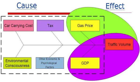
1.3 RESEARCH SCOPE

There are certain critical variables which constantly change traffic volume in the real

world. However, this study attempts to focus on detecting the short-run Granger causality

and the co-integration of long-terms causal relationship between “gas price and freeway

traffic” and between “GDP and freeway traffic” only. For a clear picture of the research

scope, please find Figure 1.1, 1.2 and 1.3.

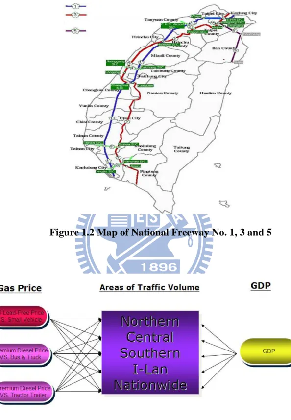
Figure 1.2 Map of National Freeway No. 1, 3 and 5

Figure 1.3 The Study of Relationship between Variables in this

Research

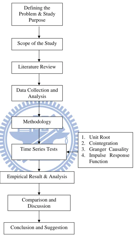
1.4 RESEARCH PROCEDURE

Within throughout this paper, the following steps and research procedures are taken. The

steps of the process are illustrated in Figure 1.4.

1. Collect and describe the data of monthly average fuel prices of 95 unleaded gas price

and premium diesel price based on the data provided by CPC Corporation, Taiwan.

2. Convert the nominal quarterly GDP data into a monthly basis deflating it into real

terms while taking into account the Consumer Price Index (CPI) (2006 = 100) of the

given period of time.

3. Compare and analyze the freeway toll traffic volume on National Freeway No. 1, 3

and 5 in a timeframe from 2004:01 to 2009:06 reported by Taiwan Area National

Freeway Bureau, MOTC.

4. Cluster the said collected traffic data into five separate categories by geography:

northern, central, southern Taiwan, I-Land area and nationwide to identify the

regional characteristics of toll traffic volume variance in different areas in reflecting

Figure 1.4 Research Flow

Literature Review

Data Collection and Analysis

Empirical Result & Analysis

Comparison and Discussion

Conclusion and Suggestion Defining the

Problem & Study Purpose

Scope of the Study

Time Series Tests Methodology 1. Unit Root 2. Cointegration 3. Granger Causality 4. Impulse Response Function

CHAPTER 2 LITERATURE REVIEW

Does X really cause Y? This time-honored issue has puzzled the great minds of

philosophers of ancient Greek, China and India for over 3000 years. “This seemingly

simple question has challenged some of the greatest thinkers in history, including

Heraclitus, Plato, Aristotle, Galileo, Hobbes, Hume, Kant, and countless other

philosophers and scientists.” (Dowd and Town 2002) But the old issue is now unfolded

again with new ideas to help unveil the mystery of causality from a different point of

view by Clive W.J Granger.

Granger, Nobel Prize laureate of Economics in 2003, established a set of techniques

named Granger Causality test to uncover the mystery and enhance our understanding of

causality to a certain degree. For example, if a variable X Granger-causes Y if Y can be

better predicted using the histories of both X and Y than it can using the history of Y

alone. To put it simply, it does not imply true causality but a statistical way for

determining whether one time series is useful in forecasting another. (Granger 1969).

As the real world is much more complicated than a set model, this thesis sets the

philosophical questions aside while focusing on the causality examination by adopting

Granger’s statistical theory. With regard to more detailed Granger causality technique,

there are more in depth discussions in the later part of the chapter - 5.3. In the current

chapter, we will present certain published on the factors affecting driving choice behavior,

traffic caused by gas price or GDP.

2.1 FACTORS AFFECTING DRIVING CHOICE BEHAVIOR

Jou and Sun (2008) apply logistics regression model to analyze how commuters and

non-commuters response to the rising oil price in Taipei. Their results indicate that when

personal income and travel cost increase, the frequency of driving car decreases. They

also discover the factors behind the auto commuter’s choice of car, which include the oil

consumption efficiency of car, the frequency of car usage and a willingness to switch to

public transportation.

Boarnet and Sarmiento (1998) adopt travel daily data for southern California residents to

study the link between road-use patterns at the neighborhood level and non-work trip

generation from a sample of 769 individuals. Their results show that the land-use

variables are statistically insignificant, thus a link between road land use and travel

behavior is inconclusive.

Cullinane (2002) cites Hong Kong as an example of how a good public transport system

can discourage car ownership. That is, the better the quality of public transportation is,

the lesser, the people want to own a car. His results, based on a survey of 389 university

students in Hong Kong, show that good public transport can deter car ownership, with

Based on the concept that users’ response to toll charges is instrumental to government

policy- making, Odeck and Brathen (2008) study elasticity of travel demand and users’

attitudes towards tolls in 19 Norwegian road projects. They discover a mean short-run

elasticity at -0.45 while -0.82 for the long-term. Furthermore, the study reveals that the

road type and project location can vary the elasticity.

Kitamura (1989) uses a sample obtained from the Dutch National Mobility Panel survey

to examine the causal structure underlying household mobility. His findings suggest that

car ownership is strongly associated with mode of transportation while it has no influence

on weekly personal trip generation by household members. He studies the characteristics

of mode through a causal analysis of changes in car ownership, number of drivers,

number of car trips and number of transit trips. His results show that observed changes in

mode use is unable to be explained by assuming that a change in transit use influences car

use. It suggests that the increase in car use, which is the result of increasing car

ownership, may not be suppressed by improving public transit.

2.2 IMPACT OF GAS PRICE SHOCKS ON TRAFFIC

Unarguably, one of the world’s most important economic energy sources, gasoline is

critical to global economic growth. The cost of gasoline constitutes a major component of

the total cost of driving. Under such assumption, rises in automobile gasoline prices

According to a survey of over 500 residents in Austin Texas focusing the aftermath of

a severe spike in gas prices that took place in September of 2005, Bomberg and

Kockelman (2007) examines how respondents’ travel behavior changed during and

following the spike. The authors use basic descriptive statistics and employ ordered

probit and binary logit models to determine which factors are responsible for behavioral

changes in response to gas price spikes. Based on the feedback from respondents, it is

indicated a strong tendency to reduce overall driving and/or a car- pool like activities in

more efficient tours as a way of coping with high oil prices.

Lu et al (2008) utilizes Grey relation analysis (GRA) to evaluate the relative influence of

the fuel price, the gross domestic product, the number of motor vehicles and the vehicle

kilometers of travel (VKT) per energy increase in Taiwan. Their finding shows that the

relationship between energy requirement and the number of passenger cars declined

steadily. The authors conclude that the steady growth of economic development is

strongly correlated with vehicular fuel consumption. The relation grade of 0.967 implies

that the increase in the number of passenger cars is another important factor for energy

increase.

Liddle (2009) embraces US data from 1946 to 2006 to examine whether a systemic,

mutually causal and cointegrated relationship exists among mobility demands, gasoline

price, income and vehicle ownership. He finds that those variables co-evolve in a

transport systems and thus, they can not be easily disentangled in the short-run. On the

because of the efficacy of the Corporate Average Fuel Economy standards (CAFE) of

influence fleet fuel economy. His analysis shows that the fuel standard program was

effective in improving the fuel economy of the US vehicle fleet and in temporarily

lessening the impact on fuel use of increased mobility demand.

2.3 IMPACT OF GDP PRICE INNOVATION ON TRAFFIC

Stern (1993) examines the causal relationship between GDP and energy use for the

period 1947-90 in the United States. He carries out a VAR of GDP, energy use, capital

stock and employment to test for Granger causal relationships between the variables. It’s

pointed out there is no evidence that energy use Granger causes GDP.

Ramanathan (2001) uses the concepts of cointegration and error correction to study the

long-run relationships between variables representing transport performance and other

macro-economic variables in India. The results demonstrate that passenger-kilometres

(PKM) in India are likely to increase faster than gross domestic product (GDP), and still

much faster than urbanisation. By the same token, tonne-kilometres (TKM) is probably

to increase faster than the index of industrial production. Besides, there are strong

correlations between TKM and industrial growth. Both the passenger and freight

performances are relatively lack of elasticity in price changes. The error correction model

(ECM) interprets that both passenger and tonne-kilometres adjust to their respective

long-run equilibrium at a moderate rate, with about 35% of adjustment in PKM and 40% of

Coondoo and Dinda (2002) present a study of income – CO2 emission causality based

on a Granger causality test, using a cross-nation panel data on per capita income and the

corresponding per capita CO2 emission data. It is indicated that three different types of

causality relationship holding for different country groups. For the developed country

groups of North America, Western and Eastern Europe, the causality is found to run from

emission to income. For the country groups of Central and South America, Oceania and

Japan causality from income to emission is obtained. As to the country groups of Asia

and Africa the causality is found to be bi-directional.

Wu (2006) indicates the ownership of vehicles and growth of its usage are related to the

increasing of GDP. She applies Granger causality and forecast error variance

decomposition techniques to examine the cointegration and causality between GDP and

the number of registered cars in Taiwan and Japan. Her results show that the causality

between GDP and car is from GDP of the number to registered car in Taiwan while in

Japan the 2 variables are independent.

Xu, Li et al (2007) based on time series data study the relationship between the freeway

transportation and the economic development through cointegration theory and Granger

causality test method. They put different periods into account and obtain there is no

relationship between the tested variables from 1978 to 1991 while there was harmonious

Getzner (2009) studies the environmental impacts of passenger transport, especially CO2

emissions from private car use in Austria. The results of the empirical estimations are

interpreted as a driving force of income with respect to car use is very strong while

technological developments fall significantly short of reducing car use. Oil price shock

brings a significantly negative but temporary effect. He even points out given the current

trends of income, and assuming the empirically indicated functional form of the

mobility/emission-income relationship, the scenarios show that even in the case of a

complete stop to any further road construction and an increasing fuel price despite an

annual increase in fuel taxes, passenger transport and private car use will still increase by

CHPATER 3 METHODOLOGY

This chapter is divided into six sections to present the methodologies adopted in this

study. The methodology of unit root, choosing the lag length for unit root test,

cointegration, vector autoregression model, Granger causality, and impulse response

function are discussed as followings.

3.1 UNIT ROOT

In time series models in econometrics, often ordinary least squares (OLS) is used to

estimate the slope coefficients of the autoregressive model. The use of OLS relies on the

stochastic process being stationary. It means the error term must be time-invariant, that is,

white noise. In other words, the necessary and sufficient condition for time series stability

is the entire characteristic roots lie within the unit circle while the condition for

nonstationarity is the entire characteristic roots lie in or outside the unit root.

When the data-generating process (DGP) is non-stationary, the use of OLS can produce

invalid estimates. Granger and Newbold (1974) called such error estimates - spurious

regression results: high R2 values and high t-ratios yielding results with no economic meaning. If the process has a unit root, one can apply the difference operator to the series.

OLS can then be applied to the resulting (stationary) series to estimate the remaining

slope coefficients. For example, if a series Yt is I(1), the series ∆Yt = Yt − Yt − 1 is I(0)

3.1.1 The Test of Unit Root

In statistics and econometrics, there are several ways to test whether time series is with a

unit root, such as the Dickey-Full, augmented Dickey-Fuller (Dickey and Fuller 1979;

Said and Dickey 1984) or the Phillips-Perron (Phillips 1987; Phillips and Perron 1988)

among others.

3.1.1.1 Dickey-Fuller unit root test (DF)

Dickey-Fuller unit root test uses the OLS to run the regression on the following three

forms and check whether δ=0 is statistically significant.

1. no drift and trend:

∆Yt =

γ

Yt-1 + et (1)

2. with drift:

∆Yt = α +

γ

_µYt-1 + et (2)

3. with drift and deterministic time trend:

∆Yt = α + βT + γτYt-1 + et (3)

Where α is intercept,

γ

/

γ

_µ/ γ_τ is auto-regression term, βT is time trend term and et

In each case, the hypotheses is:

H0: γ =0,

γ

_µ=0 or γ_τ=0 (unit root, stationary)

H1: γ ≠0,

γ

µ≠0 or γτ≠0 (without unit root, non-stationary)

If the null hypothesis - H0 is rejected, it’s concluded that the rejection of the tested

variable existing unit root. The Dickey Fuller test is only valid for AR (1) (first order

autoregressive) processes. If the time series is correlated at higher lags, the augmented

Dickey Fuller test constructs a parameter correction for higher order correlation, by

adding lag difference of the time series. More details are presented in chapter 3.1.1.2.

3.1.1.2 Augmented Dickey and Fuller Unit Root Test (ADF)

If the et has an autocorrelation for more than one period, the unit root test can be

modified as

∑

= − −

+

∆

+

+

+

=

∆

k i t i t j t t

T

Y

Y

e

Y

1 1

λ

ρ

β

α

(4) where α is a constant, β the coefficient on a time trend,

ρ

the auto-regression term and k

the lag order of the autoregressive process. Impose the constant α = 0 and β = 0 corresponding to modeling a random walk and use the constraint β = 0 corresponds to modeling a random walk with a drift. Consequently, there are three main versions of the

By including lags of the order i the ADF formulation allows for higher-order

autoregressive processes. This means that the lag length i has to be determined when

applying the test. One possible approach is to test down from high orders and examine

the t-values on coefficients. An alternative approach is to examine information criteria

such as the Akaike information criterion, Bayesian information criterion or the

Hannan-Quinn information criterion.

The null hypothesis is functioned as the DF test (i.e., H0: γ =0 for example). It is so

called Augmented Dicky-Fuller (ADF) test.

The test procedure is firstly run the unrestricted model and obtains RSSUR.

∑

= − −

+

∆

+

+

+

=

∆

k i t i t j t t

T

Y

Y

e

Y

1 1

λ

ρ

β

α

(5) Secondly, run the restricted model and obtains RSSR

∑

= −

+

∆

+

+

=

∆

k i t i t j t

T

Y

e

Y

1

λ

β

α

(6) Then compute the F-statistic as:

) /( 2 / ) ( * k n RSS RSS RSS F UR UR R − − =

Compare F to the critical values Φ that are tabulated by Dicky-Fuller (1981). The null hypothesis:

H0: ρ=0 (unit root, non-stationary)

3.1.1.3 Phillips–Perron Unit Root test (PP)

Although, ADF test is the most common way for unit root test, it does not allow having

autoregressive residuals with heteroscedasticity in the disturbance process of the test

equation. To overcome such restrictions, the Phillips-Perron (PP) test offers an alternative

method for correcting for serial correlation in unit root testing. In general, it makes a

non-parametric correction to the t-test statistic to capture the effect of autocorrelation present

when the underlying autocorrelation process is not AR(1) and the error terms are not

homoscedastic.

There are also three types of Phillips-Perron unit root tests as follows:

(1) type with zero mean

t t

t Y

Y =

α

₋₁ +

µ

(7)

(2) type with single mean

t t

t Y

Y =

µ

+

α

₋₁ +

µ

(8)

(3) type with constant and time trend term

t t

t Y t

Y =

µ

+

α

₋₁+

δ

+

µ

(9)

where µt is the innovations process.

The above three types are computed based on autoregressive model. Same as ADF test, if

the null hypothesis is rejected, it means the tested variable is stationary series without

In some conditions, the PP test tends to be more powerful than ADF test but, on the other

hand, similar to ADF, it also suffers potentially severe finite sample power (DeJong John,

David et al. 1992; Chen 2009) and suffers from severe size distortions(Schwert 1989;

Chen 2009). Size problem: actual size is larger than the nominal one when

autocorrelations of

µ

_t are negative, and therefore, are more sensitive to model misspecification (the order of autoregressive and moving average components). We can

plot ACF to help us detect the potential size.

Even though a variety of alternative procedures have been proposed that try to resolve

these problems, particularly - the power problem, there are new drawbacks in them as

well. (Maddala and Kim 1998) That’s the reason the ADF and PP tests continue to be the

most widely used unit root tests.

3.2 CHOOSING THE LAG LENGTH FOR THE UNIT ROOT TEST

An important practical issue for the implementation of the unit root test and vector

autoregressive (VAR) model is the specification of the lag length p. Sun and Ma (2004)

point out there are some commonly used procedures to chose the lag length of a VAR

system. One of them is called the ‘general-to-specific’ approach, which starts from a

maximum lag length and then testes down the significance of the longest lags. Ng and

Perron (1995) finds out there is some empirical evidence that this approach has a high

probability of over-fitting the true model. On the contrary, the approach of ‘specific to

significant extra lagged variables added in. “Both approaches involve testing the causal

variables implicitly, which may created a pre-test bias.” Sun and Ma (2004)

Different from above mentioned two approaches, explicit statistical criteria as if Akaike’s

information criterion (AIC), Schwarz’s Bayesian information criterion (SBC) are as well

frequently used for lag length selection. As AIC and SBC are well-known, the definition

of each is presented without further discussions:

AIC = ln

Σ

~

+ T

2

(number of freely estimated parameters), (10)

and SBC = ln

Σ

~ + T T ln

(number of freely estimated parameters) (11)

where Σ~ = estimated covariance matrix and T= number of observations.

If p is too small then the remaining serial correlation in the errors will bias the test while if p is too large then the power of the test will suffer. Monte Carlo experiments suggest it is better to error on the side of including too many lags. Hall (1994) and Ng and Perron (1995) also improved under some restriction, SBC tends to select a more optimal lag length. (Reimers 1992; Phylaktis 1999; Yau and Nieh 2003; Xu Hai-cheng 2007)

3.3 COINTEGRATION

This section briefly introduces the concepts of cointegration. The biggest problem with differencing is that lose valuable long term information in the data. One possible

alternative solution to this is cointegration methods which get long run solutions from non stationary variables. The definitions of cointegration given by Engle and Granger are listed as follows.

Definition 1.

Engle and Granger (1987): If a series yt with no deterministic components, can be

represented by a stationary and invertible ARMA process after differencing d times, the

series is integrated of order d, that is, y_t～I(d).

Definition 2.

Engle and Granger (1987): If all elements of the vector yt are I(d) and there exists a

cointegrating vector β≠0 such that β ' y_t～I(d-b) for any b > 0, the vector process is

said to be cointegrated CI (d,b).

The reduction in the order of integration implies a special kind of relationship with interpretable and testable consequences. Cointegration is an econometric property of time series. If two or more series are themselves non-stationary, and a linear combination of them is stationary, then the series are said to be cointegrated.

As indicated cointegration is alinear combination of 2 variables - X and Y or more series

which are non-stationary, then the series are said to be cointegrated. In other words, if they are I(k) series and may be co-integrated becoming stable process of I (k-b, b>=1), it is called the I(k) series are cointegrated. (Engle and Granger 1987; Yang 2009)

It is often said that cointegration is a mean of correctly testing hypotheses concerning the relationship between two variables having unit roots (i.e. integrated of at least order one). It means a series is said to be "integrated of order d" if one can obtain a stationary series by "differencing" the series d times.

In practice, co-integration is used for such series in typical econometric tests, but it is more generally applicable and can be used for variables integrated of higher order. However, these tests for co-integration assume that the co-integrating vector is constant during the period of study. In reality, it is possible that the long-run relationship between the underlying variables change (shifts in the co-integrating vector can occur). The reason for this might be technological progress, economic crises, changes in the people’s preferences and behavior accordingly, policy or regime alteration, and organizational or institutional developments. This is especially likely to be the case if the sample period is long.

3.3.1 The test of Cointegration

3.3.1.1 The Engle and Granger two-step procedure

The Engle and Granger two-step procedure is a residual based test. Given two variables of interest, the first step of the Engle-Granger procedure involves the estimation of the following statistic cointegrating regression:

t t t t

Y = +d βX +ε for t=1, 2, …, T (12)

intercept plus linear trend (α + βt). In the second stage, possible cointegration between

the series is examined via analysis of the order of integration of the residuals ｛ε)_t｝

from (12) using a Dickey-Fuller test as below.

2 2 1 ( 1) t t t b ρ b₋ v ∆ = − + (13)

The null of no cointegration (H0: ρ − 1 = 0) is tested via the t-ratio of (ρ− 1).

3.3.1.2 Johansen Maximum Likelihood Method

Another approach named maximum likelihood (ML) method proposed by Johansen (Johansen 1988; Johansen 1991) can be also used to analyze long-run equilibrium relationship or cointegrating vectors. There are two statistics to take into account - the trace and maximum eigenvalue. Johansen’s methodology takes its starting point in the vector autoregression (VAR) of order n given by

1 1 2 2 ....

t t t n t n t

Y =A Y₋ +A Y₋ + +A Y₋ +ε (14)

where Y is lag length n (_t p×1) vector endogenous variable. The VAR model of the first

difference can be re-written as follows:

1 1 n t j t j t n t j Y

π

Y

π

Y

ε

− − − = ∆ =

_∑

∆ + + (15)

where π_j is a short term adjusting coefficient to describe short-term relationship,

π

is

long term innovation vector that includes long term information hint in the regression to test those variables’ whether existence long term equilibrium relationship or not.

Meanwhile rank of

π

decides the number of cointegrated vector.

π

has three kinds of style:

a. rank( )π =n, then

π

is full rank. It means all of variables are stationary series in

the regression (Y ) _t

b. rank( )π =0, then

π

is null rank. It means variables do not exist cointegred

relationship.

c. 0<rank( )π = <r n, then some of variables exist r cointegrated vector.

Johansen approach has used rank of

π

to distinguish the number of cointegrated vector.

In other words, to examine rank of vector means to test how many of non-zero of characteristic roots existence in the vector. Two different likelihood ratio tests listed in equtations (16) and (17) respectively.

a. Trace test:

0 1

: ( ) (at most r integrated vector) : ( ) (at least r+1 integrated vector)

H rank r H rank r π π ≤ > 1 ˆ ( ) ln(1 ) n trace i i r r T λ λ = + = −

_∑

− (16)

T is sample size,

λ

ˆ_i is estimated of characteristic root. If test rejects H₀ that means

variables exist at least r+1 long term cointegrated relationship.

b. Maximum eigenvalue test

:

0 1

: ( ) (at most r integrated vector)

: ( ) (at least r+1 integrated vector)

H rank r H rank r π π ≤ >

max( ,r r 1) Tln(1 ˆr 1)

λ

+ = − −

λ

+ (17)

If the null hypothesis is accepted, it means variables have r cointegrated vector. The method is starting to test from variables do not have any cointegrative relationship which

is r=0. Then it adds the number of cointegrative item until H₀ can’t be rejected, which

means variables have r cointegrated vector.

3.4 VECTOR AUTOREGRESSION MODEL (VAR)

Vector autoregression (VAR) is an econometric used to capture the interrelation of time series and the dynamic impacts of random disturbances (or innovations) on the system of variables. All the variables in a VAR are treated symmetrically by including for each variable an equation explaining its evolution based on its own lags and the lags of all the other variables in the model. The main uses of the VAR model are the impulse response analysis, variance decomposition, and Granger causality tests.

A VAR model describes the evolution of a set of k variables (called endogenous variables) over the same sample period (t = 1, ..., T) as a linear function of only their past evolution.

The variables are collected in a k × 1 vector yt, which has as the ith element yi,t the time t

observation of variable yi. The mathematical representation of a VAR is:

where yt is a k x 1 vector of endogenous variables, c is a k × 1 vector of constants

(intercept), A1…, AP are matrices of coefficients to be estimated and et is a k × 1 vector

of error terms that may be contemporaneously correlated but are uncorreclated with their own lagged values as well as uncorrelated with all of the right-hand side variables.

In the VAR model, all the variables used have to be of the same order of integration. As a result, we have the following cases:

• All the variables are I(0) (stationary): one is in the standard case, ie. a VAR in

level.

• All the variables are I(d) (non-stationary) with d>0:

o The variables are cointegrated: the error correction term has to be included

in the VAR. The model becomes a Vector Error Correction Model (VECM) which can be seen as a restricted VAR.

o The variables are not cointegrated: the variables have first to be

differenced d times and one has a VAR in difference.

The information criteria can be used to choose the optimal lag length in a VAR(p) by allowing a different lag length for each equation at each time and choosing the model with the lowest AIC, SBC or other information criteria value.

3.5 GRANGER CAUSALITY

In Granger’s point of view, a universally acceptable definition of causation to this subtle and difficult concept may well not be possible, but a definition that seems reasonable to

many is : “Let Ωn represent all the information available in the universe at time n.

Suppose that at time n optimum forecasts are made of Xn+1 using all of the information

in Ωn, and also using all of this information apart from the past and present values Yn-j,

j≥0, of the series Yt,. If the first forecast, using all the information, is superior to the

second, than the series Yt, has some special information about Xt, not available elsewhere, and Yt, is said to cause Xt.” (Ashley, Granger et al. 1980)

According to Freeman (1983), for the most simple bivariate case, Granger causality can

be operationalized in the following way: Consider the process〔Xt, Yt〕, which we will

assume to be jointly covariance stationary. Denote by X_t and Y_t all past values of X and

Y, respectively. Let all past and present values of these two variables be represented as

t

X and Y_t . Define σ2( X_t│ Z ) as the minimum predictive error variance of X_t given Z,

where Z is composed of the sets 〔Xt, Yt,Xt,Yt〕. Then there are four possibilities:

1. : Y causes X: σ2 ( X_t│Y_t, X_t) < σ2 ( X_t│ X_t). 2. : Y causes X instantaneously: σ2( X_t│Y_t, X_t ) < σ2( X_t│Y_t,X_t). 3. : Feedback: σ2( Xt│Xt , Yt) < σ 2 ( Xt│ Xt), and σ2 ( Y_t│Y_t, X_t) < σ2( Y_t│Y_t).

4. : Independence: X and Y are not causally related:

σ2 ( Xt│Yt, Yt) =σ 2 ( Xt│Xt, Yt) =σ 2 ( Xt│Xt), and σ2 ( Y_t│Y_t, X_t) =σ2( Y_t│Y_t, X_t) =σ2( Y_t│Y_t).

For instance, in case I the minimum predictive error variance for Xt is smaller when the

past values of Y, Y_t, are included than when the minimum predictive error variance is

calculated solely on the basis of X_t. When the preceding result obtains and, at the same

time, X Granger causes Y, we have feedback or case III. However, it must be certain that implicit in this formulation is the presumption that there are no omitted variables that are responsible for the variations in X and Y.

3.5.1 Approaches to test Granger Causality

Here we present two approaches of Granger causality test. The discussions of them for determining Granger causality applied in this research are reported in 3.5.1.1 and 3.5.1.2.

3.5.1.1 The “Direct Granger Method”

The reason to name this method as direct is that it assesses Granger causality in a direct way: by regressing each variable on lagged values of itself and others. When both series are deemed I(0), a VAR model in levels is used. When one of the series is found I(0) and the other one I(1), VAR is specified in the level of the I(0) variable and in the first difference of the I(1) variable. When both series are determined I(1) but not cointegrated, the proper model is VAR in terms of the first difference. Finally, when the series are cointegrated, we can use a vector error correction model (VECM) or, for a bivariate system, a VAR model in levels.

The direct approach is based on the following VAR system: Yt=β0 +

∑

= J j 1 β jYt− j+

∑

= k k 1 γk Xt− k+ut, (19)

Where Yt are stationary (or can be made stationary by differencing), β0 is a constant

term, β j and γk are coefficients of exogenous variables, and ut are white noise error

terms.

We can then simply use an Ftest (Wald test) or the like to examine the null hypothesis

-γk = 0 by regressing each variable on lagged values of itself and the other. This method

produces results sensitive to the choice of lags J and K; insufficient lags yield auto-correlated errors (and incorrect test statistics), while too many lags reduce the power of the test. This approach also allows for a determination of the causal direction of the relationships, since we can also estimate the “reverse” model:

Xt=β0 +

∑

= J j 1 β jXt− j+

∑

= k k 1 γk Yt−k +ut (20)

Also, it is important to remember that Granger causality testing should take place in the context of a fully-specified model. If the model isn’t well specified, “spurious” relationships (Granger and Newbold 1974) may be found, despite the fact of no actual (conditional) relationship between the variables.

3.5.1.2 The Toda and Yamamoto Granger Causality Test

As the direct Granger causality test mentioned in 3.5.1.1 relies heavily on the results of pre-testing of unit root and cointegration. There are chances incorrect conclusions drawn from preliminary analyses or pretest biases might be carried over onto the causality test.

As a result, in order to avoid the pre-test bias, we present the Toda and Yamamoto approach as followings. Like the name suggests, it is proposed by Toda and Yamamoto (1995). In fact, it’s a modified Wald (MWald) test for linear restrictions on some parameters of an augmented VAR (mlag + d) in levels, where d is the maximum order of

integration that we suspect might occur in the process. In the bivariate case, this model

without deterministic terms can be written as follows, (Konya 2004)

y

_t =

α

₁+

∑

= mlag i 1

β

1i

y

_t−i+

∑

+ + = d mlag mlag i 1

β

1i

y

_t−i+

∑

= mlag i 1

γ

1i

x

i t− +

∑

+ + = d mlag mlag i 1

γ

1i

x

i t− +

ε

1t (21)

x

t =

α

2+

∑

= mlag i 1

β

2i

y

_t−i+

∑

+ + = d mlag mlag i 1

β

2i

y

_t−i+

∑

= mlag i 1

γ

2i

x

i t− +

∑

+ + = d mlag mlag i 1

γ

2i

x

i t− +

ε

2t (22)

where the most important is that VAR model can be cointegrated or non-cointegrated. The variables in the VAR may be either stationary or non-stationary. The testing procedure explained by Sun and Ma (2004) is given as follows.

“Suppose the lag length is chosen as q by the SIC and the maximum order of the integrated time series is one. We estimate a VAR with q+1 order and then only apply the Wald test on the coefficients of the variables with lags up to q to conduct the Grager causality test”. (Lutkepohl and Burda 1997)

Except the advantage of being free from the pre-test bias, there is one more advantage of this MWald method based on the study of Zapata and Rambaldi (1997). They perform Monte Carlo experiments on bivariate and trivariate models, and get the results showing that the surplus lag test has excellent finite sample properties for both cointegrated and non-cointegrate VAR models.

3.6 IMPULSE REPONSE FUNCTION

Impulse Response Function (IRF) traces the effect of an innovation in one variable on the

others. For example, let Y_t be a k-dimensional vector series generated by

1 1 ... t t p t p t Y =A Y₋ + +A Y₋ +U (23) 1 ( ) t t i t i i Y B U U ∞ − = = Φ =

∑

Φ (24) 2 1 2 ( ... _p p) ( ) I = −I A B−A B − −A B Φ B (25)

where cov(Ut) =Σ, Φi is the MA coefficients measuring the impulse response. In a

detailed and exact way, Φjk,i represents the response of variable j to a unit impulse in

variable k occurring ith period ago. As Σ is usually non-diagonal, it is impossible to

shock one variable with other variables fixed. Some kind of transformation is needed. Cholesky decomposition is the most popular one which we shall turn to now. Let P be a

lower triangular matrix such that Σ= PP', then Eq. (24) can be rewritten as

0 t i t i i Y θ ω ∞ − = =

_∑

(26)

where θi = Φiωt = P-1Ut and E(ωtωt’)=I. Let D be a diagonal matrix with same diagonals

with P and W = PD-1, Λ =DD'. After some manipulations, we obtain

Yt = B0Yt + B1Y t-1 + · · · + BpY t-p + V t (27)

where B0= Ik −W-1, W = PD-1, Bi = W-1Ai. Obviously, B0 is a lower triangular matrix with

0 diagonals. In other words, Cholesky decomposition imposes a recursive causal structure from the top variables to the bottom variables but not the other way around.

For a K-dimensional stationary VAR(p) process, φjk,i = 0, for j ≠ k, i=1,2,… is equivalent

to φjk,i=0, for i=1,…, p(K-1). That is to say if the first pK−p responses of variable j to an

impulse in variable k is zero, then all the following responses are all zero. (Lutkepohl

CHPATER 4 DATA COLLECTION AND ANALYSIS

4.1 THE DATA

This section discusses and analyzes the time series variables to be utilized in the later chapter. In this study, the monthly historical gas price data is obtained from the prices offered by CPC, Corporation, as it enjoys a 78% & 77% market share respectively (EpochTimes Taiwan 2008) in the supply of 95 lead-free gasoline and premium diesel gasoline.

A country’s GDP, which generally reflects the development of national economy, is chosen as the second index of a factor affecting traffic volume. We collect the quarterly real GDP data published by Directorate General of Budget, Accounting and Statistics,

Executive Yuan, R.O.C. The data has been adjusted by Consumer Price Index (CPI) of

2006 and converted to monthly basis using it as a measurement of ability to support a car’s carrying cost.

One might expect the impact of gas price and GDP on traffic volume to be more significant when they are calculated in real terms. Therefore the gas price time series data are computed by dividing the nominal price by the ratio of 2006 CPI announced by Directorate General of Budget, Accounting and Statistics, Executive Yuan, R.O.C. to real terms (100 in 2006) in order to eliminate the influence of the inflations.

The original data of National Freeway No. 1, 3, and 5 monthly toll station traffic volumes are taken from Taiwan Area National Freeway Bureau, MOTC. Based on the preliminary data the traffic of each station is categorized into 5 clusters according to geographical locations. We obtained traffic volumes in four areas – northern, central, southern, and I-Lan area plus the one throughout the island.

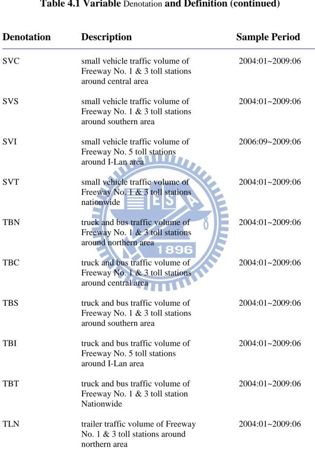
The period of each variable computed in this study falls between 2004:01 to 2009:06, yielding a total of 66 monthly observations for each vehicle type. The toll traffic volume in I-Lan area, on the other hand, is taken from the period between 2006:09 to 2009:06 as it opened its service in 2006. Table 4.1 contains a list of the variables analyzed in this study.

Table 4.1 Variable Denotation and Definition

Denotation Description Sample Period

R95P real 95 lead-free gas price 2004:01~2009:06

(NT$ per liter, price adjusted based on 2006 Taiwan Consumer Price Index)

RDSP real premium diesel price 2004:01~2009:06

(NT$ per liter, price adjusted based on 2006 Taiwan Consumer Price Index)

RGDP real gross domestic product 2004:01~2009:06

(million NT$, seasonally adjusted at 2006 price)

SVN small vehicle traffic volume of 2004:01~2009:06

Freeway No. 1 & 3 toll stations around northern area

Table 4.1 Variable

Denotation

and Definition (continued)

Denotation Description Sample Period

SVC small vehicle traffic volume of 2004:01~2009:06

Freeway No. 1 & 3 toll stations around central area

SVS small vehicle traffic volume of 2004:01~2009:06

Freeway No. 1 & 3 toll stations around southern area

SVI small vehicle traffic volume of 2006:09~2009:06

Freeway No. 5 toll stations around I-Lan area

SVT small vehicle traffic volume of 2004:01~2009:06

Freeway No. 1 & 3 toll stations nationwide

TBN truck and bus traffic volume of 2004:01~2009:06

Freeway No. 1 & 3 toll stations around northern area

TBC truck and bus traffic volume of 2004:01~2009:06

Freeway No. 1 & 3 toll stations around central area

TBS truck and bus traffic volume of 2004:01~2009:06

Freeway No. 1 & 3 toll stations around southern area

TBI truck and bus traffic volume of 2004:01~2009:06

Freeway No. 5 toll stations around I-Lan area

TBT truck and bus traffic volume of 2004:01~2009:06

Freeway No. 1 & 3 toll station Nationwide

TLN trailer traffic volume of Freeway 2004:01~2009:06

No. 1 & 3 toll stations around northern area

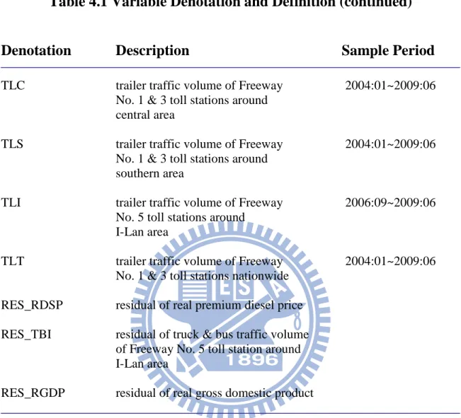
Table 4.1 Variable Denotation and Definition (continued)

Denotation Description Sample Period

TLC trailer traffic volume of Freeway 2004:01~2009:06

No. 1 & 3 toll stations around central area

TLS trailer traffic volume of Freeway 2004:01~2009:06

No. 1 & 3 toll stations around southern area

TLI trailer traffic volume of Freeway 2006:09~2009:06

No. 5 toll stations around I-Lan area

TLT trailer traffic volume of Freeway 2004:01~2009:06

No. 1 & 3 toll stations nationwide

RES_RDSP residual of real premium diesel price

RES_TBI residual of truck & bus traffic volume

of Freeway No. 5 toll station around I-Lan area