國
立
交
通
大
學
資訊科學與工程研究所
碩
士
論
文
程序層級上耗電參數與公式的校正
Calibrating Parameters and Formula for Process-level Energy
Consumption Profiling
研 究 生:尤云千
指導教授:林盈達 教授
程序層級上耗電預估參數與公式的校正
Calibrating Parameters and Formula for Process-level Energy
Consumption Profiling
研 究 生:尤云千 Student:Yun-Chien Yo
指導教授:林盈達 Advisor:Dr. Ying-Dar Lin
國 立 交 通 大 學
資 訊 科 學 與 工 程 研 究 所
碩 士 論 文
A Thesis
Submitted to Institute of Computer Science and Engineering College of Computer Science
National Chiao Tung University in partial Fulfillment of the Requirements
for the Degree of Master in Computer Science June 2010 Hsinchu, Taiwan
中華民國九十九年六月
I
程序層級上耗電預估參數與公式的校正
學生: 尤云千 指導教授: 林盈達
國立交通大學資訊科學與工程研究所
摘要
搭載電池的移動式裝置經常受到能源上嚴格的限制。程序階級上的耗能分析 工具可以找出系統中最耗能源的程序,並且可以仔細地分析出個別硬體元件的耗 能情形。利用這樣的工具,軟體開發工程師可以分析與微調各程序的電能消耗, 藉此來提高電池的使用時間。不過這種耗能分析工具經常綁定特定的硬體,所以 需要為各個硬體平台來做耗能分析工具的校正。此外,對於新加入的硬體元件也 需為其創造新的耗能預估公式。這篇論文提出一個兩階段式的方法來校正產品上 的耗能分析工具。第一階段利用數位電表來重新建立屬於新產品的耗能功率表。 第二階段則是使用線性回歸分析來創造新的耗能預估公式。在五種情境下驗證的 結果顯示,經過我們校正之後耗能分析工具的預測錯誤率都低於 10%。此外,我 們發現 FTP 上傳與下載的程序雖然消耗的電能不同,但是花在 CPU 計算與網路傳 輸的耗能比例卻是一樣的。 關鍵字: 耗能分析,耗能預估校正,AndroidII
Calibrating Parameters and Formula for Process-level Energy
Consumption Profiling
Student: Yun-Chien Yo Advisor: Dr. Ying-Dar Lin
Department of Computer and Information Science
National Chiao Tung University
Abstract
The battery-powered mobile devices get tight constrains on energy resources. The process-level energy profiling tools can identify the most energy-consuming process and detail the energy usages of each hardware component. With the help of energy profiling tools, programmers can fine-tune the energy consumption of processes to improve the battery lifetime. However, the profiling tools are highly hardware dependent and therefore require to be calibrated for each hardware platform. Besides, new energy estimation formulas need to be created for new hardware components. In this thesis, a two-phase calibrating approach is proposed to handle the two issues on off-the-shelf product devices. The first phase reconstructs the power table with a power meter, and the second phase creates new energy estimation formulas with the linear regression analysis. The accuracy of the calibrated tool is evaluated under five scenarios with the error ratios proven below 10%. Moreover, the energy consumption of FTP upload and download processes is different but the ratio of CPU computing energy to networking energy is the same.
III
Contents
CHAPTER 1. INTRODUCTION ... 1
CHAPTER 2. BACKGROUND ... 4
2.1 Spectrum of Energy Consumption Studies ... 4
2.2 Energy Consumption of Wireless Network Interface ... 7
2.3 Battery Use in Android Systems ... 8
CHAPTER 3. PROBLEM STATEMENT ... 11
3.1 Terminologies ... 11
3.2 Problem Description ... 11
CHAPTER 4.TWO-PHASE CALIBRATION APPROACH ... 14
4.1 Calibration Approach Overview ... 14
4.2 Power Table Reconstruction ... 16
4.3 New Formula Creation ... 17
4.4 Example Run of Two-phase Calibration ... 21
CHAPTER 5. IMPLEMENTATION ON ANDROID DEV 1 ... 23
5.1 Power Table Reconstruction on Dev 1 ... 23
5.2 Wi-Fi Formulas Creation on Dev 1 ... 25
5.3 Wi-Fi Power Daemon Implementation on Dev 1 ... 27
CHAPTER 6. EVALUATION STUDIES ... 29
6.1 Evaluation Framework ... 29
6.2 Evaluation Scenarios without Networking ... 31
6.3 Evaluation Scenarios with Networking ... 33
IV
List of Figures
Fig. 1. Energy estimation overview. ... 2
Fig. 3. Architecture of Android system. ... 9
Fig. 4. Backlight energy consumption behaviors of smartphones. ... 14
Fig. 5. Tow-phase calibrating flowchart. ... 16
Fig. 6. Example run of two-phase calibration. ... 21
Fig. 7. Power consuming behavior of Wi-Fi interface. ... 25
Fig. 8. Linear regression of Wi-Fi module in operation modes. ... 26
Fig. 9. Wi-Fi power daemon implementation. ... 28
Fig. 10. Power consumption evaluation framework. ... 29
Fig. 11. Energy consumption under system idle scenario. ... 31
Fig. 12. Energy consumption under CPU intensity scenario. ... 32
Fig. 13. Energy consumption under web browsing scenario. ... 33
V
List of Tables
Table 1. Comparison of software energy profiling tools. ... 7
Table 2. Default energy estimation formulas in Battery Use. ... 10
Table 3. Terminology definitions. ... 11
Table 4. Power table values comparison. ... 24
Table 5. Linear regression results summarization. ... 27
1
Chapter 1. Introduction
The processing speed of microchips doubles every two years, i.e., Moore’s law [1], while the battery capacity only doubled in the last ten years [2]. Battery-powered mobile devices, such as smartphones, with plenty of computing-intensive applications, e.g. music play program and GPS navigation, and energy-hungry peripherals, e.g., screen and Wi-Fi module, especially suffer from the shortage of energy budgets. Because of the lack of accurate energy profiling tools on product devices, application programmers are usually good at performance optimization but relatively lack sense of energy fine-tuning. As the result, the energy profiling tools are demanded and studied over the past several years.
Related works studying energy consumption of a system can be classified into three approaches: measurement approach, simulation approach, and estimation approach. Measurement approach measures energy consumption with digital power meters directly. One can either sample total power under different configuration factors, e.g. processor frequency, to identify the influence of such the factors on system power consumption [3], or probe all hardware components simultaneously to get energy consumption of each component in detail [4-6]. Furthermore, mapping the measured energy consumption onto running processes helps programmers detect energy-hungry code regions [7-10]. Simulation approach creates virtual hardware platforms to simulate energy consumption behavior for energy profiling [11-12]. Based on system resource utilization gathered from the hardware emulator, the energy consumption of the simulated platform can be calculated. Estimation approach is similar to simulation one except it collects the resource utilization information from kernel and log daemons at profiling time. Some researches based on this approach achieve software energy profiling [13-14] and online power-saving adaptation [15-16] without the need of power meters.
2
Measurement approach is intuitive and accurate. However, a product device for costing down and size reduction usually removes the reserved pins required for power meters. Developing an energy-aware simulator for every new hardware platform is also impractical. As a result, the estimation approach becomes a complementary solution for software energy profiling on product devices.
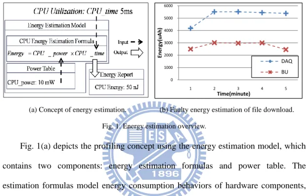
(a) Concept of energy estimation. (b) Faulty energy estimation of file download. Fig. 1. Energy estimation overview.
Fig. 1(a) depicts the profiling concept using the energy estimation model, which contains two components: energy estimation formulas and power table. The estimation formulas model energy consumption behaviors of hardware components, and the power table contains the power weight coefficients of the formulas. While the profiling time, each record of resource utilization is logged for calculating the energy consumption of each process on hardware components. For example, in Fig. 1(a), the CPU utilization, CPU_time, logged for the profiled process is 5 ms. According to the CPU energy estimation formula and the power weight coefficient, CPU_power, the CPU energy consumed by profiled process is 50 nJ.
Although the estimation approach looks into process level on product devices without power meter support, the energy estimation formulas and the power table are heavily hardware dependent. Therefore, default power table in primitive source code of an energy estimation program, e.g. Android Battery Use (BU), has to be customized for a device under test (DUT) first. Besides, in a porting procedure, faulty
0 1000 2000 3000 4000 5000 6000 1 2 3 4 5 Ene rg y(uA h ) Time(minute) DAQ BU
3
energy estimation formulas harming the estimating accuracy seriously also have to be addressed. Fig. 1(b) shows a dramatic discrepancy between the energy estimation of BU and the energy measurement of Data Acquisition (DAQ) [17], where X axis denotes the n-th minute and Y axis denotes aggregate energy consumed in the minute. The inaccurate estimation results from the faulty energy estimation formula for the Wi-Fi module in the primitive source code.
In this work, on product devices, a two-phase calibration approach is proposed to calibrate the default power table parameters and the faulty energy estimation formulas. The first phase focuses on reconstructing the power table and the second phase details creating estimation functions for target hardware components. Our approach evaluates on Android smartphones, i.e. gphone, because of the open source characteristics of Linux kernel and Android application framework.
The rest of this thesis is organized as follows. Chapter 2 reviews the ways to investigate energy consumption on variant devices and introduces the Android framework together with the built-in energy estimation program, Battery Use. Beside, the energy consumption studies about WLAN interface is included for the background of system implementation. Chapter 3 states terminologies and problem statements. Chapter 4 describes the concept of our approach, two- phase calibration, along with an example run. Chapter 5 shows the detail operation procedures and the system implementation on an Android product device. Chapter 6 presents the evaluation results, and finally, chapter 7 concludes the thesis.
4
Chapter 2. Background
This chapter investigates the spectrum of energy consumption studies, introduces the energy consumption behaviors of WLAN interface, overviews the experiment Android platform together with our evaluation target, Battery Use.
2.1 Spectrum of Energy Consumption Studies
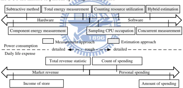
Seven methods of the measurement and estimation approaches are introduced. For distinction, hardware and software energy consumption are discussed separately. The relationship between software and hardware energy consumption is analogous to the commerce in a market, as shown in Fig. 2. DUT and hardware components on it are analogous to a market and stores in the market separately. Processes running on the DUT are likened to persons spending in the market.
Total energy measurement
Hardware Software
Market revenue Personal spending
Power consumption Daily life expense
Component energy measurement
Subtractive method Counting resource utilization Hybrid estimation
Sampling CPU occupation Concurrent measurement
Total revenue statistic
Income of store Amount of spending
Count of spending rough
detailed detailed
Measurement approach Estimation approach
Fig. 2. Spectrum of energy consumption studies.
Hardware Energy Consumption
Based on the resolution of energy breakdown, the three methods, total energy measurement, subtractive method, and component energy measurement, are generalized.
Total energy measurement, which observes the energy consuming behaviors from the total energy consumption, is like examining the business status from the total
5
revenue of the market. On handheld computers, Assim [3] measured the total energy consumption in different system configurations, and showed that energy consumption of display, processor, and Wi-Fi module plays important roles in determining battery lifetime.
Subtractive method roughly identifies the component-wide energy consumption by comparing energy consumption differences in variant hardware status. Component energy measurement simultaneously probes on each hardware component to sample the energy consumed by the components and can be illustrated with setting up invoice machines to keep track of incomes for each store. On portable computers, Bai and Lin [5] presented the energy measurement method for hardware components with the small resisters. Mahesri and Vardhan [6] measured energy consumption of main hardware components on IBM laptop. Mahesri and Vardhan’s study concluded that the power consumed by CPU and display, again, dominates the power consumption of laptop; and the hardware components, i.e. disk drivers, consume large energy only in the working state.
Software Energy Consumption
According to the accuracy of energy attribution, the methods for examining software power consumption are classified into four methods, i.e. sampling CPU occupation, counting resource utilization, hybrid estimation, and concurrent measurement.
In practice, sampling CPU occupation samples total energy with an external power meter. In order to map the measured energy onto the processes running on the DUT, the meter also triggers the logs of a program counter (PC) and a process identifier (PID) for each energy record. In the analysis time, the energy record can be attributed to the exactly one process according to the PC and the PID. Because the energy-to-process mapping only depends on CPU occupation, the inaccurate energy
6
attribution is raised by concurrent energy consumption of hardware components. With this manner, PowerScope [7] is the most famous tool for discovering the energy-hungry code regions. Chang et al. [8] replaced the time-driven sampling approach of PowerScope with an energy-driven sampling approach to improve accuracy of energy attribution. ePRO [9] integrates energy and performance profiling into a convenient tool with well-defined user interface.
In order to trace software energy consumption on each hardware component, counting resource utilization method counts resource requests for each process. The counts of resource requests can be translated into energy consumption using the energy estimation model mentioned in the chapter 1. For daily life analogy, the method works like counting each kind of receipts for personal spending estimation. In [15], pTop estimates component-wide energy consumption for each process on laptop and provides programming interface for designing energy-aware applications. ECOSystem [16] counts resource utilization and allocates energy budgets among competing tasks carefully to extend battery lifetime.
Hybrid estimation method is a derivation of counting resource utilization and sampling CPU occupation. In practice, some of the resource utilization can be counted easily, e.g. disk I/O, while the other resource utilization is hard to be counted on the DUT, e.g. memory access. The energy consumed by the countable resources is easy to be estimated, while the residual energy escaped from estimation shall be shared proportionally according to the CPU occupation. Using the hybrid estimation method, PowerSpy [14] roughly distinguishes the battery energy consumed by threads and some hardware components.
Concurrent measurement embeds energy sensors on hardware components to trace energy utilization simultaneously. For accurate energy attribution, it introduces a sophisticated manner for synchronizing the multisource energy samples and the
7
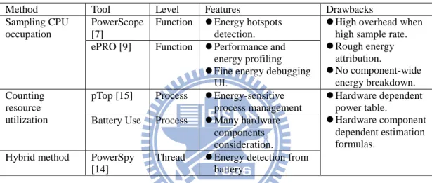
system events. For analogy, it is like keeping track of each spending for persons in the stores. The amount spending of a person can be calculated by summing up the price of his or her bills. Xian et al. [10] proposed an accurate energy attribution which raises the accuracy by up to 90% over sampling CPU occupation. Table 1 summarized the comparisons of tools for software energy profiling. This thesis focuses on calibrating the energy estimation tools of counting resource utilization method by handling the two hardware dependent drawbacks.
Table 1. Comparison of software energy profiling tools.
Method Tool Level Features Drawbacks
Sampling CPU occupation
PowerScope [7]
Function Energy hotspots detection.
High overhead when high sample rate. Rough energy
attribution.
No component-wide energy breakdown. ePRO [9] Function Performance and
energy profiling Fine energy debugging
UI. Counting
resource utilization
pTop [15] Process Energy-sensitive process management Hardware dependent power table. Hardware component dependent estimation formulas.
Battery Use Process Many hardware components consideration. Hybrid method PowerSpy
[14]
Thread Energy detection from battery.
2.2 Energy Consumption of Wireless Network Interface
The energy efficiency of WLAN interface is a significant issue especially for battery-powered mobile devices. Therefore, for a clean image of power consumption behaviors, M. Stemm and R. Katz [18] measured the power consumption on four distinct interfaces. They concluded that power consumption of receiving packets almost equals the power consumption of idle network interface, and sending packets cost more power consumption than receiving packets. Ebert et al. [19] further studied on the influence of packet size, transmission rate, and RF power level on power consumption of 802.11 standard network interfaces. In an identical RF channel, Ebert et al. showed that higher RF power level results in more power consumption on the interface. On the other hand, the packet size and the transmission rate play minor roles
8
in power consumption. For mathematical analysis, L. M. Feeney and M. Nilsson [20] characterize the energy consumption of an IEEE 802.11 wireless network interface operating in an ad hoc mode as simple linear formulas. However, the work did not include the discussion of power saving mechanism, which contains two distinct operation modes, power saving mode (PS) and active mode (AM). In PS, the interface awakes from the sleep state only for beacon packets periodically and consumes a little energy. On the contrary, in AM, the interface keeps active in the idle state for handling instantaneous packet transmission, so it consumes an additional power inherently. In [21], C. Rohl et al. simulate the power saving mechanism of an IEEE 802.11 ad hoc wireless network. From the simulation, they also identified the figures for optimum beacon intervals an ATIM window sizes.
2.3 Battery Use in Android Systems
At the end of 2008, Android, a new software platform for smartphones, was released by Google. The market share of Android is expected to keep growth in the next few years [22].
Android Framework
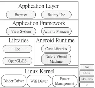
Android takes Linux kernel as hardware abstraction because it provides lots of proven hardware drivers and sophisticated core operating system infrastructures especially in the networking layers. Upon the OS, lightweight libraries, e.g., Bionic libc, optimized for embedded system are exposed for native programming. Dalvik virtual machine and core libraries, which provide most of the functionality for Java programming, construct the runtime environment for Android applications. Application framework contains several services to serve the user applications. Take the advantage of Dalvik virtual machine and unified application framework, applications can migrate between platforms seamlessly. According to the functionality and performance consideration, each portion of Android is created in different
9 languages, as shown in Fig. 3.
Browser Battery Use Application Layer
Application Framework View System Activity Manager Libraries Aneroid Runtime
Core Libraries libc OpenGL/ES Dalvik Virtual Machine Binder Driver Linux Kernel
Wifi Dirver Power Management
Java C/C++ C/C++/Java
C
Fig. 3. Architecture of Android system.
Battery Use
Battery Use is an energy consumption estimation program which belongs to counting resource utilization method and is embedded in Android system since version 1.6. During system booting, the application framework starts a special service, battery info, to take responsibility for the counting resource utilization. For the energy consumption calculating, Battery Use raises the inter process communication (IPC) to pull the data from the battery info service.
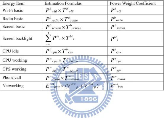
Table 2 summarizes the default energy estimation formulas and power weight coefficients in Battery Use. In the table, each kind of the basic energy is energy consumption used for keeping hardware component active and each kind of the working energy results from that a hardware component works for one or many processes. In the basic energy estimation formulas, PbR is basic power consumption
of hardware component R, and TbR is the time duration wherein the component is
active. Because there are many brightness levels, backlight energy estimation is formulated in a summation form of multiple energy consumption instances. In the estimation formulas of working energy, PwR is working power and TwR,p is the
10
duration wherein hardware component R is working for process p . The networking energy estimation of process p is defined as a product of per byte transmission energyEnetbyte and total traffic volume including receiving packets
p rcv
V and sending packets Vsndp.
Table 2. Default energy estimation formulas in Battery Use.
Energy Item Estimation Formulas Power Weight Coefficient Wi-Fi basic Pbwifi Tbwifi Pbwifi
Radio basic PbradioTbradio bradio
P Screen basic PbscreenTbscreen bscreen
P Screen backlight
I i i i bt i bt T P bti PCPU idle
P
bcpu
T
bcpu PbcpuCPU working PwcpuTwcpu,p Pwcpu
GPS working PwgpsTwgps,p Pwgps
Phone call PwradioTwradio Pwradio Networking Enetbyte(Vrcvp Vsndp) Enetbyte
11
Chapter 3. Problem Statement
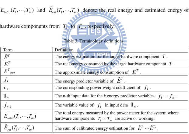
3.1 TerminologiesTable 3 defines the common terminologies used in this thesis. Real energy consumption of target hardware component T is E and is estimated by T EˆT. EˆT is formulated by energy predictor variable fk together with its power weight coefficient ck. For linear regression analysis, I is the n-th input data set which n
contains k values fn,1 to fn,k for the predictor variable f1 to fk. Because E T
is hard to be measured directly on product devices, ETapx, the approximate value, is
taken in the regression analysis for creating a new estimation formula. )
, ,
( 1 m
total T T
E and Eˆest(T1,,Tm) denote the real energy and estimated energy of
hardware components from T1 to T , respectively. m
Table 3. Terminology definitions.
Term Definition
T
Eˆ The energy estimation for the target hardware component T.
T
E The real energy consumed by the target hardware component T.
apx T
E The approximate energy consumption of ET.
k
f The energy predictor variable of T Eˆ .
k
c The corresponding power weight coefficient of fk.
n
I The n-th input data for the k energy predictor variables f 1 fk. k
n
f , The variable value of fk in input data In. )
, , ( 1 m
total T T
E The total energy measured by the power meter for the system where hardware components
m
T
T 1 are active or working. ) , , ( ˆ 1 m est T T
E The sum of calibrated energy estimation for EˆT1EˆTm.
3.2 Problem Description
On produce devices, direct energy measurement on hardware component is not possible because there are not reserved pins for probing. Moreover, there is no reason to expect achievement of component-wide energy measurement which can only be completed with evaluation boards. Therefore, in this work, energy consumption
12
measurement is only performed for the system total energy at the battery, and the criterion for the evaluation procedures is based on the total energy instate of per component energy bias. With this constrain, the following describes the calibration problem statements.
Let the consumed energy E for a component T T be modeled as a linear equation EˆT c.0c1f1ckfk containing k energy predictor variables and k+1 power weight coefficients. c is the constant parameter and 0 c is the corresponding k
coefficient of energy predictor variable f . The thesis calibrates the faulty energy k
estimation by solving two problems: default power table parameters and faulty energy estimation formulas.
Problem statement 1: Default Power Table Parameters
The default power table parameters problem is to update the power weight coefficients stored in the default power table, such that the estimation error
new c T T err E E E ˆ _
between estimated energy consumption
k k new c T f c f c c Eˆ _ .0 1 1 and real energy is minimized.
Problem statement 2: Faulty Energy Estimation Formulas
The faulty energy estimation formulas problem is to model the energy consumption for component T by creating a linear equation with
k k new f T f c f c c Eˆ _ '.0 1 1 , such that the estimation error
new f T T err E E E ˆ _
13
14
Chapter 4. Two-phase Calibration Approach
This chapter details the two-phase calibration methodology on product devices. The first phase reconstructs a power table for DUT and the second phase creates an energy estimation formula for hardware components with regression analysis.
4.1 Calibration Approach Overview
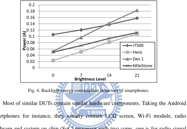
Fig. 4. Backlight energy consumption behaviors of smartphones.
Most of similar DUTs contain similar hardware components. Taking the Android smartphones for instance, they usually contain LCD screen, Wi-Fi module, radio hardware and system on chip (SoC) processor with two cores, one is for radio signal processing and another is for user applications. Because energy consumption heavily depends on hardware components, equipping the similar hardware components usually makes the DUTs follow resemble energy consumption behaviors. For example, as shown in Fig. 4, the backlight power of the four smartphones keeps the similar linearity between brightness levels and consumes stable energy within the brightness levels. The main difference of the four lines is the slope which is related to the power weight coefficient, 𝑃𝑏𝑡𝑖, in the screen energy estimation formula mentioned in chapter 2. The observation above suggests that most of energy estimation models can adapt to similar DUTs by updating power weight coefficients for each estimation formula. 0 0.02 0.04 0.06 0.08 0.1 0.12 0.14 0.16 0.18 0.2 0 7 14 21 Pow e r (A) Brightness Level i7500 Hero Dev 1 MileStone
15
In practice of power table reconstructions, two categories of power consumption are generalized: system-basic power and process-related power. The system-basic power is used to activate hardware components. The process-related power is consumed by hardware components which are working for processes. In our definition, the energy consumption from the system-basic power belongs to the entire system, while the energy consumption from the process-related power shall be charged from the corresponding processes.
Even if hardware components of DUTs are similar, some of the energy estimation formulas still cannot be successfully applied to the new DUT because of the variant specification of hardware component T. In order to create new energy estimation formulas to replace the faulty one, a linear regression analysis is introduced to help modeling power consumption behaviors of T. However, on the product DUT, real energy E consumed by T T is unable to be directly measured for
the regression analysis because there are no longer reserved pins for measurement. Alternatively, approximate energy consumption ETapx is presented for the
substitution of E in the regression analysis. Finally, for the programmers’ convince, T
the energy estimated by new formulas is mapped onto running processes for process-level energy profiling.
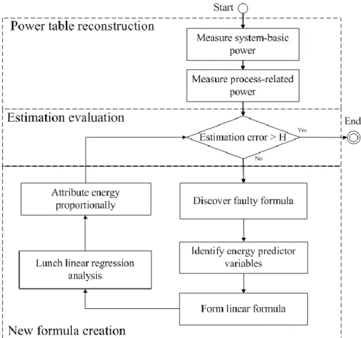
Fig. 5 depicts the main flowchart of the two-phase calibration which contains the estimation evaluation and the two calibrating phases, i.e. power table reconstruction and new formula creation. The first phase, power table reconstruction, is divided into two function blocks measuring the system-basic power and the process-related power separately. Between the two phases, the estimation evaluation is used to feeding back calibrated results. There are predefined test scenarios and a threshold (H ) for evaluation procedure. The calibrated tools will be tested by estimating energy
16
consumption of each test scenario. If one of the estimation errors is larger than the threshold H, the procedure of second phase will be performed for further calibration. In the thesis, the error ratio, defined in chapter 6, is chosen as the criteria. The second phase, new formula creation, includes the creating of new estimation formulas and a proportional manner used to distribute the estimated energy fairly.
Fig. 5. Tow-phase calibrating flowchart.
4.2 Power Table Reconstruction
System-basic power coefficient measurement
It is easy to obtain the system-basic power weight coefficient, e.g. 𝑃𝑏𝑤𝑖𝑓𝑖, by measuring the difference of total power consumption while the hardware component operates in different states. The most common case is to measure the power difference between on and off states of hardware components. In other cases, multiple power measurement is performed when the target component can be configured into several
17
operating states. For example, screen backlight can work in multiple brightness levels and results different power consumption in the each level, as shown in Fig. 4.
Process-related power coefficient measurement
Because the process-related power, e.g. Twcpu,p, depends on the hardware
resource utilization, a dedicated process is used to stress the hardware component. In practice, the dedicated process should be chosen or designed carefully for stressing only one hardware component at a time. For instance, the infinite for-loop can be used to stress CPU hardware component with minimized memory accesses. The process-related power can be refined by subtracting the total system-basic power from the measured total power consumption. It is the reason why the process-related power measurement shall follow the system-basic power measurement.
4.3 New Formula Creation Discovering faulty formula
From the feedback of estimation evaluation, there may be a faulty estimation formula which brings out the incorrect energy estimation results because of containing wrong energy predictor variables or omitting significant predictor variables, which characterize the unequal energy consumption behaviors for the new DUT. Therefore, the faulty estimation formula always makes the faulty results on T, no matter how the power weight coefficients are modified. The following presents a simple manner to discover the only one faulty formula on the DUT. Let there are m estimation formulas each for a hardware component and there is only one faulty formula among the estimation formulas. Under such situation, there can be C test km scenarios each involving k hardware components, where k is arbitrary variable and smaller than m. During the evaluation under test scenarios, two false evaluations scenarios can be found and both of them involve the faulty estimation formula. With
18
the cross-matching manner, the m joint formulas of both false evaluation scenarios can be extracted. Based on the m formulas, the next loop is continued with Ckm
test scenarios until the only one joint formula is discovered. At the end of the discovering procedure, the only one joint formula is the faulty estimation formula.
Identifying energy predictor variables
For determining the energy predictor variables for T, a series of experiments shall be held to observe the significant effect of each candidate energy predictor variable fk on energy consumption. In each experiment, only one energy predictor variable can be examined with different variable values. Another possible way for finding out the energy predictor variables is to take the advantage of proven results from the papers which studied deeply on the power consumption behavior of T on
the similar hardware platform. However, this step is tough and requires the domain knowledge of T for the energy predictor variable choice.
Forming linear formulas
As the assumption in [15, 23], it assumes that the linear property between hardware resource utilization and energy consumption of T is held. Therefore, the estimation
equation is formulated in a summation form,
k k T f c f c c Eˆ .0 1 1 , where fk is the new energy predictor variable and ck is its corresponding power weight coefficients.
In order to train the unknown k+1 coefficients, the observation input data I is n
collected together with the instance of real energy consumption ETn consumed by
T. For the convenience of regression analysis, the relationship of input data set F, the real energy consumption set ET
ET1 ET2 ETn
T , and power weight19
coefficient set C
c0 c1 ck
T are compiled in a vector formFC
ET
where the matrix of input data set F is shown as
k n n k k n f f f f f f , 1 , , 2 1 , 2 , 1 1 , 1 2 1 1 1 1 I I I F .
In practice, the influence of energy predictor variables on energy consumption shall not always be first-order. However, the leaner regression also can handle formulas containing higher than first-order predictor variables, such like
2 2 2 1 1 0 . ˆ c c f c f ET .
The vector form for regression analysis can be denoted as
2 1 0 2 2 , 1 , 2 2 , 2 1 , 2 2 2 , 1 1 , 1 2 1 1 1 1 c c c f f f f f f E E E n n n T T T .
Launching linear regression analysis
Unfortunately, because the reserved pins for component-wide energy measurement have been removed, the real energy T
E cannot be measured directly from hardware component T with power meter. The alternative is applying the
approximate energy consumption ETapx for ET. Assume there are totally m+1
active or working components during measuring the total energy and energy estimation of m components performs well after the first phase calibrating. Therefore, the ETapx is calculated by a subtracting operation,
) ,... ( ˆ ) , ,... ( 1 m est 1 m total apx T T T E T T T E E ,
20 ) , , , (T1 T T
Etotal m is measured total energy of m+1 hardware components.
In practice, the trick is that the calibrating procedure of T only can be
performed after the energy consumption of other involved hardware components can be estimated. For instance, before calibrating energy consumption of the networking module, the CPU energy consumption shall be estimated well because the networking packages always consume the energy on CPU for network protocol processing. Therefore, instate of T E ,
T n apx T apx T apx T apx T E E E ,1 ,2 , Eis taken as the energy consumed by T for the regression analysis, where ETapx,n is
approximate value for ETn. The solution of C is calculated as
FTF FTETapxC 1 with the least square method [24].
Attributing energy proportionally
The final work is to map the energy consumption onto the related processes causing it. Based on per-process information logging, each resource request on hardware component T is counted in the profiling time. In the analysis time, the estimated energy of the new created formula can be proportionally shared among the corresponding processes fairly according to the request counts.
21
4.4 Example Run of Two-phase Calibration
Evaluation Result Fail Scenario 1 T1 T T2 T T1 T2 Scenario 2 Scenario 3 Fail Pass Hardware component ) , , (T1 T2 T Etotal ) , ( ˆ 2 1T T Eest apx
E
T(a) Evaluation results under three scenarios. (b) Approximate energy consumption of T Fig. 6. Example run of two-phase calibration.
Assume there are three hardware components, T , T1, T2, on a DUT which is a product device without reserved pins for component-wide energy measurement, and an energy estimation application is being calibrated for correct energy estimation on the DUT. The application contains three estimation formulas, EˆTfault, EˆT1, EˆT2, and
a default power table with null values. EˆT1 estimates the system-basic energy of
1 T ,
while EˆTfault and EˆT2 predict the process-related energy of T and T2
respectively. In the first phase of the calibration procedure, the system-basic power weight coefficient of EˆT1 is retrieved with the manner of switching on and off
1 T .
For the case of EˆTfault and EˆT2 , the desired process-related power weight
coefficients are measured with two dedicated programs stressing on T and T2 individually.
After the first phase, the calibrated tool is evaluated under three (C23) scenarios. Each scenario involves different hardware components and the evaluation results are shown in Fig. 6(a). With the cross-matching manner, because T appears on both of the two failure scenarios, the EˆTfault is identified as a faulty energy estimation
22
experiments and form a new formula EˆTnew. In order to regression analysis, the
energy consumption of T is on demand and approximated by ETapx. In Fig. 6(b),
the energy consumption of T1 and T2 are correctly estimated by Eˆest(T1,T2) after
the first phase calibration, and the total energy Etotal(T1,T2,T3) can also be measured directly at the battery or the power supply. Finally, for the example of mapping
estimated energy onto processes, if in a time interval the energy estimated by EˆTnew is eT and the usage count of hardware component T is 3 and 4 time units for the processes P1 and P2 respectively. Then, the energy consumed by P1 on T is
23
Chapter 5. Implementation on Android Dev 1
In this work, the Android Dev Phone 1 (Dev 1) [25] is taken as the DUT. The goal of this chapter is to go through the two-phase calibration procedures for the correct energy estimation of Battery Use on Dev 1.
5.1 Power Table Reconstruction on Dev 1
Power consumption of eight hardware components is measured in the thesis and classified into the two categories, system-basic and process-related. The measurement procedures for each hardware component are summarized as follows.
System-basic
Wi-Fi basic: The Wi-Fi basic power is easy to be obtained by switching on and off the Wi-Fi module with Android Setting application.
Radio basic: The Airplane mode, which closes every wireless interface including the phone radio, is utilized to switch the radio between on and off state.
Screen backlight: In the Android Linux, the sysfs file system [26], which is able to set values into the kernel variables, is used to configure the screen brightness. Because of the linearity of backlight power, as shown in Fig. 4, the power difference between the maximum and minimum screen brightness is measured and denoted as Pbtmax. Power consumption of other
brightness levels is calculated with the linear interpolation.
Screen basic: The power consumed by LCD panel is obtained by measuring the power difference between the screen on and off state. In practice, there are two tricks of the screen basic power measurement. First, the screen backlight shall be turned off with the manner mentioned above for distinguishing the screen basic power from the backlight power. Second, in order to avoid the system coming into suspend mode when screen is closed,
24
the partial wakelock [27], which is a power management feature of Android system, should be acquired. The wakelock acquirement also can be done through the sysfs file system.
CPU idle: In the Battery Use, it is defined as the power consumed while screen is closed. With power button on the Dev 1, it is easy to turn off the screen.
Phone call: The power of making a call can be measured by the average power during the call and excluding the other basic power.
Process-related
GPS working: For the purpose of getting the GPS working power, the Android application, GPSTest, is created to activate the GPS hardware resource.
CPU working: CPU_busy which contains the infinite for-loop is used to stress the CPU hardware resource separately.
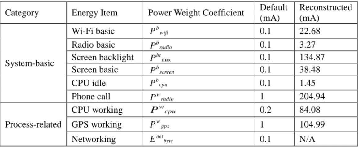
Table 4 compares the power tables from three sources. The default power table is the raw data from Android source code and the reconstructed table is rebuilt with our manner. The most energy consuming hardware is the radio component during the phone calls. Moreover, the screen backlight under maximum brightness level and the working GPS consume more power than the busy CPU..
Table 4. Power table values comparison.
Category Energy Item Power Weight Coefficient Default (mA)
Reconstructed (mA)
System-basic
Wi-Fi basic Pbwifi 0.1 22.68
Radio basic Pbradio 0.1 3.27
Screen backlight Pbtmax 0.1 134.87
Screen basic Pbscreen 0.1 38.48
CPU idle Pbcpu 0.1 1.45
Phone call Pwradio 1 204.94
Process-related
CPU working Pwcpu 0.2 84.08
GPS working Pwgps 1 104.99
25
5.2 Wi-Fi Formulas Creation on Dev 1
Form the evaluation results, the estimation errors of test scenarios involving Wi-Fi networking always exceed predefined error ratio threshold (10%). As the result, the original Wi-Fi estimation formula is recognized as the faulty formula. Therefore, the goal is to create the new estimation formula for the Wi-Fi module on Dev 1.
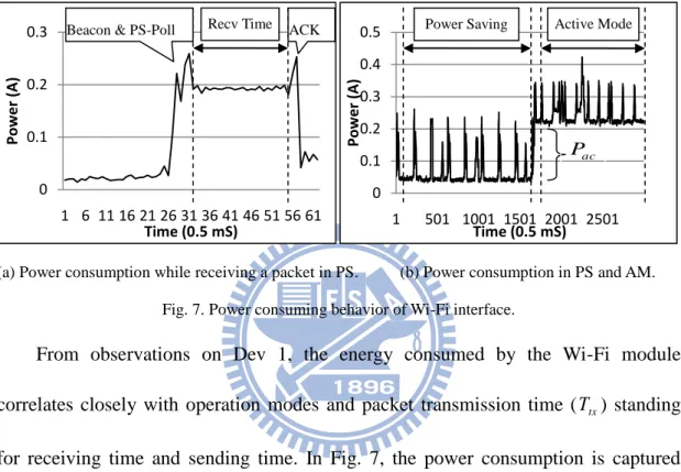
(a) Power consumption while receiving a packet in PS. (b) Power consumption in PS and AM. Fig. 7. Power consuming behavior of Wi-Fi interface.
From observations on Dev 1, the energy consumed by the Wi-Fi module correlates closely with operation modes and packet transmission time (T ) standing tx
for receiving time and sending time. In Fig. 7, the power consumption is captured from the power line of battery while receiving packets. The length of power pulse, in Fig. 7(a), closely depends on the time receiving a packet. Fig. 7(b) depicts dramatic difference in power consumption between power saving mode (PS) and active mode (AM) under the same data rate. The obviously difference is that, in AM, the Wi-Fi module consumes an active energy from active power (P ) inherently. ac
In the experiment, T is taken as the energy predictor for the Wi-Fi module. tx
The general regression equation of the module is formulated as
tx wifi T c c Eˆ 0 1 .
In order to produce different lengths of packet transmission time, user datagram 0 0.1 0.2 0.3 1 6 11 16 21 26 31 36 41 46 51 56 61 Pow e r (A) Time (0.5 mS) 0 0.1 0.2 0.3 0.4 0.5 1 501 1001 1501 2001 2501 Pow e r (A) Time (0.5 mS) Power Saving
Recv Time Active Mode
ac
P
26
protocol (UDP) packets in different sizes are transmitted with several data rates, e.g. 54 Mbps and 11 Mbps. The linear regression analysis is launched for sending and receiving packets in the two operation modes individually. The results are shown in Fig. 8 and summarized in Table 5. In Fig. 8, the high correlation coefficient (r) of
each line proves the liner property between transmission time and energy consumption of the Wi-Fi module.
(a) Regression of receiving and sending in PS. (b) Regression of sending packet in AM. Fig. 8. Linear regression of Wi-Fi module in operation modes.
In AM, because the receiving power approximately equals P , receiving the ac
packet consumes no additional energy on the Wi-Fi module excluding active energy. Therefore the receiving energy of AM is omitted from the regression analysis and estimated simply with Wi-Fi active energy Eˆwifiac shown in Table 5. The value of
ac
P is retrieved as 165.81 mA by measuring the power difference between the two
modes.
In Fig 8(a), because the sending slope is two times steeper than the receiving slope, it implies that sending one byte consumes more energy than receiving two bytes in PS. Moreover, additional energy for listening to the beacons and sending the polling control packet [19] (PS-Poll) makes the constant coefficient of the receiving line bigger than the sending line. Finally, the comparison between the sending line in
27
Fig. 8(a) and (b) suggests that sending packets consumes less energy in AM than in PS.
Table 5. Linear regression results summarization.
Mode Energy Estimation Function (uAh)
PS recv Eˆwifips_recv70.22337Trecv0.155057
send Eˆwifips_send 169.25099Tsend 0.021450
AM recv ac ac ac wifi T P Eˆ send ac ac ac wifi T P Eˆ 058923 . 0 761373 . 54 ˆ _ send send ac wifi T E recv ps wifi send ps wifi E
Eˆ _ / ˆ _ : The sending/receiving energy estimation in PS.
send recv T
T / : The sending/receiving time of a packet.
ac wifi
Eˆ : The estimated energy consumed by Pac.
ac
T : The time duration while Wi-Fi module works in AM send
ac wifi
Eˆ _ : The sending energy estimation in AM
With per-process traffic logging, the estimated transmission energy, e.g.
send ps wifi
Eˆ _ , easily relates to the corresponding processes transmitting the packets.
Because the policy of switching into AM is related to packet count, the estimated active energy Eˆwifiac is shared propositionally according to the sending and receiving
packet counts of processes.
5.3 Wi-Fi Power Daemon Implementation on Dev 1
For logging networking traffic, the socket layer of Android Linux kernel is modified slightly. In the layer, a list of recorders, which count traffic volume for each process, is created. In fact that some of the networking traffic does not consume the resource of the Wi-Fi module in the case of inter process communication (IPC). Thus, for excluding the IPC traffic from statistic, the packets with the local address, e.g. 127.0.0.1, are filtered out by a blacklist. The translation between the traffic volume and desired transmission time is achieved through the data rate information retrieved
28 directly from the Wi-Fi driver.
App App Socket TCP/UDP IP Data Link Wi-Fi Driver Wi-Fi Power Daemon proc Traffic Info Pkt Count Info Data Rate Info Log Info Network Traffic Kernel Space User Space Log File
Fig. 9. Wi-Fi power daemon implementation.
In the Wi-Fi driver, the policy of switching the operation modes is the count of the packets transmitting through the Wi-Fi module. If the packet count is more than fifteen in a second, the Wi-Fi module automatically switches into AM. If the packet count is less than eight in a second, the module will return to PS from AM. Therefore, in order to predict the operation modes for Wi-Fi module, the packet count information is captured from the data link layer.
In our implementation, as shown in Fig. 9, Wi-Fi power daemon is created in C language to reduce the performance overhead of Java virtual machine; the proc [28] files are created for shipping the information from kernel space to user space. The Wi-Fi power daemon calculates the energy consumption of the Wi-Fi module for each process and logs the results into a file once per second. In order to integrate the logs of Battery Use and Wi-Fi power daemon, a log parser is created to combine the two logs with the timestamps labeled on each energy record.
29
Chapter 6. Evaluation Studies
In this chapter, an evaluation framework is designed to verify the correctness of the energy estimation result. Moreover, the energy consumption of five evaluation scenarios is profiled in process level for case studies. In all the scenarios, the processes or hardware components dominate the energy consumption will be found out. Moreover, the ratios of networking energy to computing energy are examined in networking related scenarios.
6.1 Evaluation Framework DAQ Energy Measurement Result Energy Estimation Result B at te ry Energy Sampler Log Parser Battery Use H ar d w ar e S o ft w ar e
Device Under Test Measurement Host Machine
Machine
USB data line Current
Probe Power line
USB data line
Wi-Fi power daemon Log #1 Log #2 Dev l AP (802.11 b,g) Web/File Server
Fig. 10. Power consumption evaluation framework.
In order to evaluate the energy estimation result, the energy measurement shall be performed for reference. In this work, DAQ, NI cDAQ-9172 [29], with a current probe, LEM PR30 [30], is chosen for measuring the energy consumption from the power line extended by us between the battery and Dev 1, as shown in Fig. 10. In our experiments, Dev 1 is configured in the minimum brightness level and the SIM card is omitted. For a clean networking environment, the Wi-Fi access point (AP) and the server with FTP, ProFTPD, and web, Apache, service forms a local network. Dev 1 is configured to transmit networking traffic only through the Wi-Fi module.
30
DAQ into the energy measurement result every second. On the other hand, the energy estimation result is produced from the energy estimation daemons, i.e. Battery Use and Wi-Fi power daemon, running on Dev 1. While the profiling time, the energy sampler and the energy estimation daemons generate the measurement and the estimation logs concurrently. In the analysis time, the log parser processes the energy estimation logs migrated from Dev 1 for the energy estimation result. The accuracy of the energy estimation result is judged with the error ratio (err), which is defined as
% 100
/
est mea mea
err ,
where est is the energy estimation result, and mea is the energy measurement result. The smaller err is, the more accurate est will be.
For accuracy comparison, the full-system modeling solution presented in [23] is also implemented and the total system energy is estimated by
net disk mem cpu dev E u E u E u E u P 10.067(8.67 4) (1.28 7) (2.15 5) (3.56 4) ,
where ucpu is CPU utilization in percentage, umem is sum of data and instruction
cache miss count in kilo-time per second, udisk is number of read and write sectors,
and unet is sum of send and receive traffic volume in kilo-byte per second. However, the full-system modeling solution does not provide the energy consumption information of processes and hardware components.
Table 6 summarizes the average error ratios and the standard deviations over five experiment iterations. In the table, full-system results are energy consumption estimated by the full-system modeling solution and the two-phase results are the energy estimation created by Battery Use and Wi-Fi power daemon. Because of different estimation errors of hardware energy estimation formulas, the error ratios of the two-phase result don’t keep consistent among the five scenarios. However, the
31
estimation accuracy of two-phase results is guaranteed because all the error ratios are below 10%. On the contrary, the full-system modeling solution only performances well in CPU intensive and FTP download scenarios. It may result from that the four predictor variables of full-system estimation formula can not exactly model the energy consumption behaviors of the embedded devices including plenty of hardware components.
Table 6. Error ratio comparison under five scenarios. Without Networking With Networking System Idle CPU Intensive Web Browsing FTP Download FTP Upload Full-system Mean 24.60% 9.04% 25.80% 6.52% 34.78% Standard Deviation 2.31 2.28 1.78 1.49 0.46 Two-phase Mean 4.79% 7.39% 9.16% 2.82% 4.74% Standard Deviation 2.47 1.10 1.84 1.07 0.72
6.2 Evaluation Scenarios without Networking System Idle Scenario
(a) Estimation evaluation in system idle scenario. (b) Energy profiling in system idle scenario. Fig. 11. Energy consumption under system idle scenario.
In this scenario, the idle system of Dev 1 is measured for four minutes. Fig. 11(a) shows that the energy estimation accuracy of the two-phase result is guaranteed by a small average error ratio of 4.79%. Fig. 11(b), the pie chart depicts the energy decomposition in process level under the scenario. From the figure, the energy consumption of Dev 1 is dominated by display energy (97%) which includes the
0 200 400 600 800 1000 1200 1 2 3 4 En e rgy (u Ah ) Time(minute)
DAQ two-phase Display
97% BU 2% system 1% others 0%
32
energy consumed by the screen backlight and the LCD panel. According to the power table, Table 4, the backlight in minimum brightness is expected to consume 28% of display energy, while the screen panel consumes 72 % of the energy. However, the overhead of profiling tool is minute, because Battery Use denoted as BU only consumes 2% of total energy in Fig. 11(b).
CPU Intensive Scenario
(a) Estimation evaluation in CPU intensity scenario. (b) Energy profiling in CPU intensity scenario. Fig. 12. Energy consumption under CPU intensity scenario.
BenchmarkPi, which calculates the approximate value of Pi, is a CPU intensive application installed from the Android market. In the experiment, the BenchmarkPi is executed once and twice separately in the first and the second minute. The accuracy of energy estimation is held with average error ratio of 7.39%. Fig. 12(b) shows that BencharmkPi consumes considerable energy (41%) on CPU and the display energy (54%) still dominates energy consumption of Dev 1 in the case.
0 500 1000 1500 2000 2500 1 2 En e rg y(u A h ) Time(minute) DAQ two-phase Display 54% BU 1% Benchm arkPi 41% system 4% others 0%
33
6.3 Evaluation Scenarios with Networking Web Browsing Scenario
(a) Estimation evaluation in web browsing scenario. (b) Energy profiling in web browsing scenario.
(c) CPU and Wi-Fi module energy consumption of browser and FTP client. Fig. 13. Energy consumption under web browsing scenario.
In the following and in the pie charts, the Wi-Fi power daemon is showed as WPD for short. The test web pages located in our web server are copied from the Yahoo Taiwan website. During five minute experiment, the web page is bowered by Android default browser every forty seconds. In the Fig. 13(a), the estimation result closely matches to the measurement result with an average error ratio of 9.16%. In Fig. 13(b), again, the energy profiling tools consume negligible energy because BU together with WPD takes a small portion of energy consumption. The energy consumed by the browser is identical to the display energy. Besides, keeping the Wi-Fi module active also consumes 17% of total energy. Because the test web pages
0 1000 2000 3000 4000 1 2 3 4 5 En e rg y(u A h ) Time(minute) DAQ two-phase Display 40% Wi-Fi baisc 17% browser 39% BU 0% system 2% WPD 0% others 2% 58% 26.5% 26.5% 42% 73.5% 73.5% 0 3000 6000 9000 12000 15000 18000 21000
Web Browse FTP upload FTP download
En e rg y(u A h )
34
contain JavaScript which busies the CPU, the browser consumes more energy on the CPU (58%) than on the Wi-Fi module (42%) in the scenarios, as shown in Fig. 13(c)
File Transmission Scenarios
(a) Estimation evaluation in FTP download scenario. (b) Energy profiling in FTP download scenario.
(c) Estimation evaluation in FTP upload scenario. (d) Energy profiling in FTP upload scenario. Fig. 14. Energy consumption under file transmission scenarios.
In this experiments, a 90 MB file is transmitted between Dev 1 and the file server by a FTP client, AndFTP, Fig. 14(a) and (c) soundly shows the high accuracy of the two-phase results with average error ratios below 5%. Because sending packets consumes more energy than receiving packets, file upload application is more energy consuming than file download. From Fig. 14(b) and (d) the FTP client, andftp, is consumes about 70% energy of Dev 1 under the two scenarios. Counter to the web browser, the FTP client consumes more energy on Wi-Fi networking than on CPU computing, as shown in Fig. 13(c).
0 2000 4000 6000 1 2 3 4 5 En e rg y(u A h ) Time(minute) DAQ two-phase Display 18% Wi-Fi basic 8% BU 0% andftp 67% system 1% tiwlan_ wifi_wq 5% WPD 0% others1% 0 1000 2000 3000 4000 5000 6000 1 2 3 4 5 En e rg y(u A h ) Time(minute) DAQ two-phase Display 16% Wi-Fi basic 7% BU 0% andftp 72% system 1% tiwlan_ wifi_wq 3% WPD 0% others1%
35
Chapter 7. Conclusion and Future Works
This thesis proposes the two-phase calibration approach to adjust the faulty energy estimation results in process level on off-the-shelf product. The first phase reconstructs the power table for the DUT, and the second phase further creates the formula to replace faulty one with linear regression analysis.
In all case studies, the accuracy of energy estimation is evaluated with the error average ratios proven below 10%. Even better, the average error ratios of our calibrated results exhibit less than 5% under the file transmission scenarios. Moreover, we further show that two-phase results are more accurate than full-system results from 1.2 to 7.3 times
From the case studies, we observed that the energy consumption of display energy takes a lot portion of total energy consumption especially when the system is idle; keeping the Wi-Fi module active also consumes a considerable energy. Besides, on Wi-Fi module, sending 1 byte consumes more energy than receiving 2 bytes in power saving mode.
Finally, the overhead of our implementation, Wi-Fi power daemon and Battery Use, is proven with minor overhead below 3% upon the total energy consumption.
Because of the lack of estimation formulas for video hardware decoder, the energy profiling of video applications are not included in the evaluation scenarios. Therefore, the future extension of this work includes taking energy hungry video hardware decoder into account and profiling the energy consumption of the video applications, e.g. YouTube. Besides, the problem for discovering multiple faulty formulas also has to be addressed because there are usually multiple faulty formulas on the DUT simultaneously.