remote sensing
ArticleSediment-Mass Accumulation Rate and Variability in
the East China Sea Detected by GRACE
Ya-Chi Liu1, Cheinway Hwang1,*, Jiancheng Han1, Ricky Kao1, Chau-Ron Wu2, Hsuan-Chang Shih3and Natthachet Tangdamrongsub4
1 Department of Civil Engineering, National Chiao Tung University, 1001 Ta Hsueh Rd., Hsinchu 300, Taiwan; [email protected] (Y.-C.L.); [email protected] (J.H.); [email protected] (R.K.)
2 Department of Earth Sciences, National Taiwan Normal University, 88, Sec. 4, Tingzhou Rd., Taipei City 116, Taiwan; [email protected]
3 Department of Real Estate and Built Environment, National Taipei University, 151, Daxue Rd., Taipei City 237, Taiwan; [email protected]
4 School of Engineering, Faculty of Engineering and Built Environment, University of Newcastle, Callaghan 2308, Australia; [email protected]
* Correspondence: [email protected] or [email protected]; Tel.: +886-3-572-4739; Fax: +886-3-571-6257
Academic Editors: Xiaofeng Li and Prasad S. Thenkabail
Received: 17 June 2016; Accepted: 9 September 2016; Published: 20 September 2016
Abstract:The East China Sea (ECS) is a region with shallow continental shelves and a mixed oceanic circulation system allowing sediments to deposit on its inner shelf, particularly near the estuary of the Yangtze River. The seasonal northward-flowing Taiwan Warm Current and southward-flowing China Coastal Current trap sediments from the Yangtze River, which are accumulated over time at rates of up to a few mm/year in equivalent water height. Here, we use the Gravity Recovery and Climate Experiment (GRACE) gravity products from three data centres to determine sediment mass accumulation rates (MARs) and variability on the ECS inner shelf. We restore the atmospheric and oceanic effects to avoid model contaminations on gravity signals associated with sediment masses. We apply destriping and spatial filters to improve the gravity signals from GRACE and use the Global Land Data Assimilation System to reduce land leakage. The GRACE-derived MARs over April 2002–March 2015 on the ECS inner shelf are about 6 mm/year and have magnitudes and spatial patterns consistent with those from sediment-core measurements. The GRACE-derived monthly sediment depositions show variations at time scales ranging from six months to more than two years. Typically, a positive mass balance of sediment deposition occurs in late fall to early winter when the southward coastal currents prevail. A negative mass balance happens in summer when the coastal currents are northward. We identify quasi-biennial sediment variations, which are likely to be caused by quasi-biennial variations in rain and erosion in the Yangtze River basin. We briefly explain the mechanisms of such frequency-dependent variations in the GRACE-derived ECS sediment deposition. There is no clear perturbation on sediment deposition over the ECS inner shelf induced by the Three Gorges Dam. The limitations of GRACE in resolving sediment deposition are its low spatial resolution (about 250 km) and possible contaminations by land hydrological and oceanic signals. Potential GRACE-derived sediment depositions in six major estuaries are presented.
Keywords:East China Sea; GRACE; mass accumulation rate; sediment deposition; Yangtze River
1. Background
The East China Sea (ECS) is a marginal sea with a gently sloping continental shelf. It is surrounded by mainland China to the west, the Yellow Sea to the north and the Ryukyu Islands and Okinawa
Remote Sens. 2016, 8, 777 2 of 19
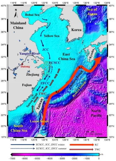
Trough to the east (Figure1). The Yangtze River, namely Changjiang or Long River, originates in the Qinghai-Tibet Plateau and flows for 6300 km eastwards to the ECS [1]. In this paper, the term Yangtze refers to the entire Yangtze River spanning from the source region in the Qinghai-Tibet Plateau to its estuary. Yangtze is the longest river in Asia and the third longest in the world; it is also the world’s leading river in sediment yield [2–4]. Yangtze’s watershed is the Yangtze basin, which is populated with a half billion people. Erosions in the Yangtze basin result in sediments that are transported to and partially deposited on the ECS shelf. The ECS also receives sediments from the Huanghe, Qiantang and Minjiang Rivers in mainland China, as well as sediments from Taiwan and elsewhere transported by the Taiwan Warm Current (TWC) and the Kuroshio Current (KC) (Figure1). As Yangtze is a major contributor of sediment deposition to the ECS [5,6], a change of sediment deposition in the ECS can be an approximate indicator for changes in rain and erosion in the Yangtze basin. A large-scale dam like the Three Gorge Dam (TGD) has been shown to reduce sediment loads in the upstream Yangtze [7]. It is likely that the TGD can also modulate the spatial and temporal patterns of sediment deposition in the ECS, but there has been no report on such potential modulations.
Remote Sens. 2016, 8, 777 2 of 19
and Okinawa Trough to the east (Figure 1). The Yangtze River, namely Changjiang or Long River, originates in the Qinghai-Tibet Plateau and flows for 6300 km eastwards to the ECS [1]. In this paper, the term Yangtze refers to the entire Yangtze River spanning from the source region in the Qinghai-Tibet Plateau to its estuary. Yangtze is the longest river in Asia and the third longest in the world; it is also the world’s leading river in sediment yield [2–4]. Yangtze’s watershed is the Yangtze basin, which is populated with a half billion people. Erosions in the Yangtze basin result in sediments that are transported to and partially deposited on the ECS shelf. The ECS also receives sediments from the Huanghe, Qiantang and Minjiang Rivers in mainland China, as well as sediments from Taiwan and elsewhere transported by the Taiwan Warm Current (TWC) and the Kuroshio Current (KC) (Figure 1). As Yangtze is a major contributor of sediment deposition to the ECS [5,6], a change of sediment deposition in the ECS can be an approximate indicator for changes in rain and erosion in the Yangtze basin. A large-scale dam like the Three Gorge Dam (TGD) has been shown to reduce sediment loads in the upstream Yangtze [7]. It is likely that the TGD can also modulate the spatial and temporal patterns of sediment deposition in the ECS, but there has been no report on such potential modulations.
Figure 1. Regional ocean circulation pattern and ETOPO1 (1 arc-minute global relief model of Earth’s surface) bathymetry around the East China Sea (ECS). The red dot shows the Datong hydrographic station; the area scattered with brown dots is the targeted area of sediment deposition near the Yangtze estuary. Abbreviations: TWC, Taiwan Warm Current; KC, Kuroshio Current; JCC, Jiangsu Coastal Current; ZFCC, Zhejiang Fujian Coastal Current; ECSCC, East China Sea Coastal Current (based on Deng et al. [5] and Liu et al. [8]).
There are two factors leading to sediment deposition on the ECS inner shelf. The first is the ECS’s wide and shallow continental shelf (500–600 km wide) that is ideal for sediments to deposit.
Figure 1.Regional ocean circulation pattern and ETOPO1 (1 arc-minute global relief model of Earth’s surface) bathymetry around the East China Sea (ECS). The red dot shows the Datong hydrographic station; the area scattered with brown dots is the targeted area of sediment deposition near the Yangtze estuary. Abbreviations: TWC, Taiwan Warm Current; KC, Kuroshio Current; JCC, Jiangsu Coastal Current; ZFCC, Zhejiang Fujian Coastal Current; ECSCC, East China Sea Coastal Current (based on Deng et al. [5] and Liu et al. [8]).
There are two factors leading to sediment deposition on the ECS inner shelf. The first is the ECS’s wide and shallow continental shelf (500–600 km wide) that is ideal for sediments to deposit.
The second is the interplay between the East China Sea Coastal Current (ECSCC) and the TWC that induces an along-shore sediment dispersal path [5]. Typically, the sediment thickness in the ECS is determined from high-resolution seismic chirp sonar profiles [8]. Previous studies on the ECS’s sediment accumulation rates and dynamics are based on a few profiles of the sediment core and inventories of radionuclide [9,10]. In general, measuring the distribution, thickness, transport, deposition and accumulation process of sediments in a given region is costly and time consuming. In coastal regions, sediment deposition can vary rapidly over space and time, making it difficult to obtain reliable sediment accumulation rates from limited sediment core samples.
The Gravity Recovery and Climate Experiment (GRACE) is a satellite mission for determining the Earth’s gravity field and its time variations [11]. GRACE has provided monthly gravity products from April 2002 to the present, which may be used to determine surface mass changes due to sources, such as sediment deposition in the ECS. Sample studies are GRACE determinations of annual hydrological variations in the Amazon basin [11], ice mass changes in Greenland and Antarctica [12,13] and groundwater depletion in India and the North China Plain [14,15]. It is commonly recognized that GRACE recovery of mass change adjacent to a land-ocean boundary can be difficult, but is possible [16]. However, the following successful GRACE studies of offshore mass changes in relatively small areas are encouraging. First, Tregoning et al. detected annual mass variations associated with sea level changes of up to ~40 cm in the Gulf of Carpentaria (~2.60×10⁵km2) [17]. Second, Wouters and Chambers detected seasonal sea level variations of up to 20 cm linked to ocean bottom pressure changes in the Gulf of Thailand (~3.15×10⁵km2) [18]. Finally, Feng et al. reported an ~18-cm mass change-induced annual variations of sea level in the Red Sea covering an area of ~4.38×10⁵km2[19]. These three examples used GRACE data and were conducted in regions with domains larger than the area corresponding to GRACE’s shortest resolving wavelength (about 250 km), but smaller than the ECS inner shelf (7.70×10⁶km2) [5]. Furthermore, the largest sediment mass accumulation rate (MAR) from sediment core measurements in the ECS corresponds to 3 cm/year in equivalent water height (EWH) changes [5]. This rate is close to the groundwater depletion rates in India and the North China Plain [14,15], thus it could be detectable by GRACE.
With the above background of the ECS sediment deposition and the GRACE capability, the objective of this study is to present a numerical algorithm for processing GRACE data to recover mass changes due to sediment deposition in the ECS. In contrast to the sparse spatial and temporal samples collected in ship campaigns [5,6], GRACE is capable of providing continuous measurements of sediment deposition at a monthly interval or even shorter. Such an improved sampling rate will allow determinations of sediment-induced mass variations at varying time scales. We will assess the GRACE-derived MARs (in terms of EWH) by data from sediment core measurements in the ECS and discuss GRACE’s limitations in resolving mass changes associated with sediment deposition.
2. Data and Method 2.1. GRACE Data
We obtained monthly gravity fields in the form of fully-normalized spherical harmonic coefficients (SHCs) generated by three official GRACE Science Data System (SDS) centres: Center for Space Research at University of Texas (CSR), the Jet Propulsion Laboratory (JPL) and GeoForschungsZentrum Potsdam (GFZ). In this paper, we used the latest version, the GRACE Release-05 (RL05), covering the period from April 2002–March 2015. RL05 has been evaluated for oceanic applications and significantly reduced noises in SHCs compared with previous releases of GRACE [16].
Since the aim of this study is detecting sediment deposition over oceans, we used both GRACE GSM (GRACE Satellite only Model) and GRACE GAD coefficients. GSM represents geopotential coefficients derived from GRACE and contain the Earth’s static gravity field and gravity variations other than the effects (background models) modelled by the three centres [20]. Table1summarizes the background models of GSM. In Table1, IERS, GOT, FES, SCEQ and EOT respectively stand for
Remote Sens. 2016, 8, 777 4 of 19
International Earth Rotation and Reference Systems Service, global ocean tide, finite element solutions, self-consistent equilibrium model and empirical ocean tide model. If the models in Table1are perfect, GSM will be free from the gravity changes caused by the underlying processes, such as ocean and solid Earth tides. Note that non-tidal oceanic and atmospheric loadings are also removed from GSM. However, our targeted area of sediment (the area around the brown dots in Figure1) is near the land-ocean boundary, where models for on-tidal oceanic and atmospheric loadings can contaminate our result. Therefore, to properly recover GRACE signals due to sediment-induced mass change in the ECS, the subtracted Atmosphere and Ocean De-aliasing Level-1B product (AOD1B)-implied signals were restored in the monthly GSM fields. AOD1B models atmospheric mass variabilities based on the Integrated Forecast System of the European Centre for Medium-Range Weather Forecasts (ECMWF) and the oceanic mass variabilities based on the ocean model for circulation and tides (OMCT). GAD is one of the AOD1B products, and it represents the ocean bottom pressure variability from the improved OMCT; it is also free from continental leakage [21].
Table 1. The modelled effects used in the GSM products from three GRACE Science Data System (SDS) centres. CSR, Center for Space Research at University of Texas; GFZ, GeoForschungsZentrum Potsdam; IERS, International Earth Rotation and Reference Systems Service; GOT, global ocean tide; FES, finite element solutions; SCEQ, finite element solutions; EOT, empirical ocean tide model; OMCT, ocean model for circulation and tides.
Effect CSR JPL GFZ
Solid Earth tide IERS-2010 IERS-2003 IERS-2010
Ocean tide GOT4.8, FES2004 GOT4.7, SCEQ EOT11a
Pole tide IERS-2010 (cubic) IERS-2003 (linear) IERS-2010 (cubic) Ocean pole tide Self-consistent equilibrium model No No
Indirect J2 effect Sun, Moon Moon Moon
Non-tidal oceanic loading OMCT (for all centres) Non-tidal atmospheric loading ECMWF (for all centres) 2.2. GRACE Determination of Mass Changes Associated with Sediment Deposition
To determine sediment-induced mass changes, we computed surface mass changes using GRACE’s monthly SHCs from the updated GSM and GAD products. Since the high-degree SHCs are corrupted by noises [22], we truncated both GSM and GAD SHCs at degree and order 60 in our computations. Several monthly SHCs from GRACE are not provided by GRACE SDS centres, and these missing values were interpolated linearly from the nearest SHCs. Figure2shows the flowchart of GRACE data processing for detecting the sediment mass change.
Remote Sens. 2016, 8, 777 4 of 19
the background models of GSM. In Table 1, IERS, GOT, FES, SCEQ and EOT respectively stand for International Earth Rotation and Reference Systems Service, global ocean tide, finite element solutions, self-consistent equilibrium model and empirical ocean tide model. If the models in Table 1 are perfect, GSM will be free from the gravity changes caused by the underlying processes, such as ocean and solid Earth tides. Note that non-tidal oceanic and atmospheric loadings are also removed from GSM. However, our targeted area of sediment (the area around the brown dots in Figure 1) is near the land-ocean boundary, where models for on-tidal oceanic and atmospheric loadings can contaminate our result. Therefore, to properly recover GRACE signals due to sediment-induced mass change in the ECS, the subtracted Atmosphere and Ocean De-aliasing Level-1B product (AOD1B)-implied signals were restored in the monthly GSM fields. AOD1B models atmospheric mass variabilities based on the Integrated Forecast System of the European Centre for Medium-Range Weather Forecasts (ECMWF) and the oceanic mass variabilities based on the ocean model for circulation and tides (OMCT). GAD is one of the AOD1B products, and it represents the ocean bottom pressure variability from the improved OMCT; it is also free from continental leakage [21].
Table 1. The modelled effects used in the GSM products from three GRACE Science Data System
(SDS) centres. CSR, Center for Space Research at University of Texas; GFZ, GeoForschungsZentrum Potsdam; IERS, International Earth Rotation and Reference Systems Service; GOT, global ocean tide; FES, finite element solutions; SCEQ, finite element solutions; EOT, empirical ocean tide model; OMCT, ocean model for circulation and tides.
Effect CSR JPL GFZ
Solid Earth tide IERS-2010 IERS-2003 IERS-2010 Ocean tide GOT4.8, FES2004 GOT4.7, SCEQ EOT11a
Pole tide IERS-2010 (cubic) IERS-2003 (linear) IERS-2010 (cubic) Ocean pole tide Self-consistent equilibrium model No No
Indirect J2 effect Sun, Moon Moon Moon
Non-tidal oceanic loading OMCT (for all centres) Non-tidal atmospheric loading ECMWF (for all centres) 2.2. GRACE Determination of Mass Changes Associated with Sediment Deposition
To determine sediment-induced mass changes, we computed surface mass changes using GRACE’s monthly SHCs from the updated GSM and GAD products. Since the high-degree SHCs are corrupted by noises [22], we truncated both GSM and GAD SHCs at degree and order 60 in our computations. Several monthly SHCs from GRACE are not provided by GRACE SDS centres, and these missing values were interpolated linearly from the nearest SHCs. Figure 2 shows the flowchart of GRACE data processing for detecting the sediment mass change.
Figure 2. A flowchart of GRACE data processing for determining sediment deposition. SHC,
spherical harmonic coefficient; GLDAS, Global Land Data Assimilation System; EWH, equivalent water height.
Figure 2.A flowchart of GRACE data processing for determining sediment deposition. SHC, spherical harmonic coefficient; GLDAS, Global Land Data Assimilation System; EWH, equivalent water height.
For the GSM product, the degree-one terms were replaced by the corresponding terms determined from geocenter variations [23], and the degree-two terms were replaced by those from satellite laser ranging (SLR) data [24]. Since north-south stripes were present in the original GRACE gravity fields due to high correlations in SHCs, the P5M8 destriping (decorrelation) filter was used to remove such correlated errors in SHCs [25,26]. In fact, we also experimented with other decorrelation filters, such as P6M10. The resulting GRACE signals are similar to those from P5M8, to the extent that the MAR signal in the targeted area is clear (brown dots in Figure1). The GSM SHCs with the new degree-one and -two terms and corrected for stripes are denoted as CGSMnm and SnmGSM. For the GAD product, we set the degree-zero and degree-one terms to zero, and the resulting GAD SHCs are denoted as CnmGADand SGADnm . The SHCs used for detecting sediment deposition are computed as:
Cnm(t) =C GSM nm (t) +C GAD nm (t) −C GLDAS nm (t) (1) Snm(t) =SGSMnm (t) +S GAD nm (t) −S GLDAS nm (t) (2)
where CGLDASnm and S GLDAS
nm are SHCs derived from the model of the Global Land Data Assimilation System (GLDAS) and are used to remove the leakage effect (see Section2.3) and t is time. The changes of SHCs, δCnm and δSnm are simply computed as δCnm = Cnm−Cmean and δSnm = Snm−Smean, where Cmeanand Smeanare the averages of Cnmand Snmover April 2002–March 2015. EWH changes are computed as [27]:
δhGRACE(θ, λ, t) = aρave
3ρw 60
∑
n=0 Wn2n +1 1+kn n∑
m=0[δCnm(t)cosmλ+δSnm(t)sinmλ]Pnm(cosθ) (3)
where θ is co-latitude, λ is longitude, a is the Earth’s mean radius, ρw is the density of water (1000 kg/m3), ρaveis the average density of the Earth (5517 kg/m3), knis the loading Love number of degree n, Pnmis the fully-normalized Legendre function of degree n and order m, Wnis the 250-km Gaussian smoothing function of degree n and δhGRACEis the EWH change.
2.3. Modelling Continental Hydrology Leakage Effect Using GLDAS
Equation (3) shows that we have applied a Gaussian smoothing filter when converting SHCs to EWHs. Conceptually, a smoothed EWH is a weighted average of the neighbouring unsmoothed values. As such, unsmoothed values over land and ocean were actually used to compute smoothed values in coastal regions [28]. Thus, the Gaussian filter leads to the so-called leakage effect that causes land gravity signals to leak into the signals in coastal regions. At the seasonal and inter-annual time scales, the amplitudes of mass changes on land are much larger than those in oceans, so that the Gaussian filter will mix oceanic gravity signals with gravity signals on land. In our case, the hydrological signal on the east coast of mainland China will be aliased into the ECS inner shelf.
The leakage effect can be reduced with the help of a global land hydrology model, as shown in many studies [12,29,30]. In this paper, we reduced land-to-ocean leakages using the GLDAS hydrology model [31]. GLDAS provides global fields of land surface states and fluxes in near-real time using satellite- and ground-based observations collected by the National Aeronautics and Space Administration (NASA) Goddard Space Flight Center (GSFC), the National Oceanic and Atmospheric Administration (NOAA) and National Centers for Environmental Prediction (NCEP) [31]. In this study, we obtained monthly GLDAS-1 products (Noah V2.7) from NASA Goddard Earth Sciences Data and Information Services Center (GESDISC). GLDAS-1 has a nominal spatial resolution of 0.25◦and is available at http://ldas.gsfc.nasa.gov/.
The GLDAS-derived SHCs are computed in the following steps. First, we calculated the summation of the average soil moisture at the four depth layers (depth from 0–10 cm, 10–40 cm, 40–100 cm and 100–200 cm) and the gridded snow EWH. Then, we obtained the global hydrological
Remote Sens. 2016, 8, 777 6 of 19
EWHs by dividing the summed soil moistures by the density of water (1000 kg/m3). Next, we converted the GLDAS-derived global hydrological EWHs to SHCs using the following equation [27]: CGLDASnm SGLDASnm = 3ρw(1+kn) 4πaρave(2n+1) w hw(θ, λ) ·Pnm(cosθ) ( cosmλ sinmλ ) sinθdθdλ (4)
where θ, λ, ρave, kn, ρwand Pnmare defined in Equation (3), hwis the GLDAS-derived hydrological EWH and CGLDASnm and S
GLDAS
nm are the GLDAS-derived SHCs. Since the hydrological EWHs are given on a regular grid, the integral is implemented by the fast Fourier transform (FFT) algorithm of Hwang and Kao [32].
The GLDAS-derived SHCs (CGLDASnm and SnmGLDAS) can also be converted to changes in EWH in coastal regions to examine the contamination of hydrological gravity signals over oceans by:
δhGLDAS(θ, λ, t) = aρave
3ρw 60
∑
n=0 Wn2n +1 1+kn n∑
m=0[δCGLDASnm (t)cosmλ+δSnmGLDAS(t)sinmλ]Pnm(cosθ) (5)
where δhGLDAS represents the GLDAS-derived leakage over ocean in terms of EWH,
δCGLDASnm =C GLDAS
nm −Cmeanand δSGLDASnm =S GLDAS
nm −Smean, where Cmeanand Smeanare the average of CGLDASnm and S
GLDAS
nm , and a, ρave, ρw, Wn, n, kn, θ, λ, t, Pnmand knare defined in Equations (3) and (4). Note that, there are alternative methods for leakage reduction, e.g., the method by Yi et al. [33]. Another issue is the scaling factor for restoring lost GRACE signals due to filtering. A widely-used technique is comparing a reference signal with the filtered signal from GRACE to determine a scale factor. The only available reference signal in the targeted area of the ECS is from Deng et al. [5]. It turns out that the magnitudes of the GRACE-derived MARs (without scaling) are close to the magnitudes from sediment-core measurements (see Section3.1). Therefore, in this paper, we decided not to apply scaling factors to the GRACE results from the three centres.
2.4. Mass Changes from GRACE and Due to Sea Level Change and Sediment Accumulation
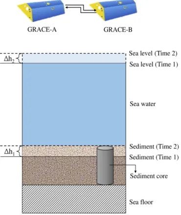
The GRACE-derived mass changes reflect the mixed effect of sediment deposition, ocean bottom pressure change (caused by sea level rise and other factors) and the replacement of sea water by deposited sediments (Figure3). In Figure3,∆h1and∆h2represent the height changes of sediment and sea level from Time 1–Time 2 (Time 2 > Time 1). The height change∆h1will not modify the sea level around the sediment, because the targeted area is very small compared to the global ocean. However, the space holding∆h1will expel existing sea water, so that here, the mass change is the sum of the positive mass of sediment and the negative mass of sea water (that is, the latter occupied the original space now filled by the sediment). The height change∆h2represents only the sea level change due to oceanic mass change, rather than the change due to oceanic thermal variations. However, not all mass-varying factors are shown in Figure3. For example, oceanic salinity change and non-tidal atmospheric change will also introduce mass changes. These effects in theory can be observed by GRACE, but separating them from the GRACE products is difficult.
The densities of the contemporarily-accumulated sediments in Figure3are hard to estimate. This is because a newly-deposited sediment takes time to consolidate, and the density will vary with time. The time-varying density of sediment is similar to that of snow. Typically, a sediment core (Figure3) taken from a research vessel is analysed in a laboratory equipped with devices to remove sea water at different sections of the core. Depending on the percentage of the removed water relative to the solid material, the density of a core section is determined. Other parameters from dating are needed to determine the rates of mass accumulation from a core. A detailed method for estimating MARs using sediment core measurements is documented in Su and Huh [9], among other works. In the literature, an MAR is the rate of mass change per unit area, and a typical unit of MAR
Remote Sens. 2016, 8, 777 7 of 19
is g/cm2/year. If we use cm/year as the unit for EWH rate and g/cm2/year as the unit for MAR, then an EWH rate (from GRACE) is numerically equal to an MAR (from sediment core). This numerical equivalence allows a fast evaluation of a GRACE result using in situ measurements of MARs like the ones presented in Deng et al. [5]. Because of the complexity in the GRACE-derived mass changes over the ECS, we interpret our result in Section3under the assumptions that (1) the mass changes due to sea level and non-tidal oceanic and atmospheric mass changes are zeroes and (2) the GRACE-derived mass change is purely due to the sediment mass without the effect of sea water replacement by the solid material of the sediment (Figure3).
core (Figure 3) taken from a research vessel is analysed in a laboratory equipped with devices to remove sea water at different sections of the core. Depending on the percentage of the removed water relative to the solid material, the density of a core section is determined. Other parameters from dating are needed to determine the rates of mass accumulation from a core. A detailed method for estimating MARs using sediment core measurements is documented in Su and Huh [9], among other works. In the literature, an MAR is the rate of mass change per unit area, and a typical unit of MAR is g/cm2/year. If we use cm/year as the unit for EWH rate and g/cm2/year as the unit
for MAR, then an EWH rate (from GRACE) is numerically equal to an MAR (from sediment core). This numerical equivalence allows a fast evaluation of a GRACE result using in situ measurements of MARs like the ones presented in Deng et al. [5]. Because of the complexity in the GRACE-derived mass changes over the ECS, we interpret our result in Section 3 under the assumptions that (1) the mass changes due to sea level and non-tidal oceanic and atmospheric mass changes are zeroes and (2) the GRACE-derived mass change is purely due to the sediment mass without the effect of sea water replacement by the solid material of the sediment (Figure 3).
Figure 3. GRACE-derived mass changes over the ECS in connection with sediment deposition, sea
level change and depletion of seawater. A sample sediment core is drilled to analyse the cumulative mass of the core.
3. Result
3.1. Sediment-Mass Accumulation: Rates from GRACE and Sediment-Core Measurements and the General Pattern
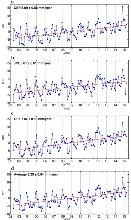
From the GRACE products, we determined monthly EWHs on a 1° × 1° grid on the ECS inner shelf. Figure 4a–c shows the three time series of monthly GRACE-derived EWHs associated with the sediment deposition from April 2002–March 2015 (156 months). The differences between the three time series are partially caused by the different background models (Table 1) in GRACE Level-2 data from CSR, JPL and GFZ. A more representative time series with less noise can be one based on the mean of the three products [34], which is shown in Figure 4d. Each of the EWH values in Figure 4 is the mean of the gridded values over 27–32°N, 122–126°E. Each of the three time series
Figure 3.GRACE-derived mass changes over the ECS in connection with sediment deposition, sea level change and depletion of seawater. A sample sediment core is drilled to analyse the cumulative mass of the core.
3. Result
3.1. Sediment-Mass Accumulation: Rates from GRACE and Sediment-Core Measurements and the General Pattern
From the GRACE products, we determined monthly EWHs on a 1◦×1◦grid on the ECS inner shelf. Figure4a–c shows the three time series of monthly GRACE-derived EWHs associated with the sediment deposition from April 2002–March 2015 (156 months). The differences between the three time series are partially caused by the different background models (Table1) in GRACE Level-2 data from CSR, JPL and GFZ. A more representative time series with less noise can be one based on the mean of the three products [34], which is shown in Figure4d. Each of the EWH values in Figure4 is the mean of the gridded values over 27–32◦N, 122–126◦E. Each of the three time series in Figure4 shows a clear rate and time-variability (oscillation). In this section, we focus on the rates inferred from the time series and discuss their variabilities in Section3.2. We least-squares fitted the monthly EWHs at each of the 1◦×1◦grids on the ECS inner shelf by a function containing a constant, the rate, annual and semi-annual cycles. The rates range from 5.61–7.04 mm/year, depending on the GRACE
Remote Sens. 2016, 8, 777 8 of 19
products (CSR, JPL and GFZ). Based on the mean of the three products (Figure4d), the rate of monthly sediment mass changes is 6.25±0.54 mm/year from April 2002–March 2015.
Remote Sens. 2016, 8, 777 8 of 19
in Figure 4 shows a clear rate and time-variability (oscillation). In this section, we focus on the rates inferred from the time series and discuss their variabilities in Section 3.2. We least-squares fitted the monthly EWHs at each of the 1° × 1° grids on the ECS inner shelf by a function containing a constant, the rate, annual and semi-annual cycles. The rates range from 5.61–7.04 mm/year, depending on the GRACE products (CSR, JPL and GFZ). Based on the mean of the three products (Figure 4d), the rate of monthly sediment mass changes is 6.25 ± 0.54 mm/year from April 2002– March 2015.
Figure 4. Monthly GRACE-derived EWHs (blue squares) over April 2002–March 2015 and rates (red
line) from (a) CSR; (b) JPL; (c) GFZ and (d) the mean of the three. An EWH is the mean of the EWHs at the grids over 122–126°E, 27–32°N (the thick black dots in the dashed boxes in Figure 5a–c).
Figure 5a–f shows the spatial distributions of rates and their standard deviations from the three GRACE products. Figure 5 shows that, for each GRACE product, the spatial pattern of the EWH rate is entirely different from that of its standard deviation, suggesting that the former is not the result of the latter. Furthermore, EWH rates peak immediately in the offshore areas of Zhejiang
Figure 4. Monthly GRACE-derived EWHs (blue squares) over April 2002–March 2015 and rates (red line) from (a) CSR; (b) JPL; (c) GFZ and (d) the mean of the three. An EWH is the mean of the EWHs at the grids over 122–126◦E, 27–32◦N (the thick black dots in the dashed boxes in Figure5a–c).
Figure5a–f shows the spatial distributions of rates and their standard deviations from the three GRACE products. Figure5shows that, for each GRACE product, the spatial pattern of the EWH rate is entirely different from that of its standard deviation, suggesting that the former is not the result of the latter. Furthermore, EWH rates peak immediately in the offshore areas of Zhejiang Province with a maximum of about 7 mm/year. In general, the spatial patterns in Figure5conform to the pattern from ground observations, which show that the sediment accumulation rate decreases with the
distance from shores and decreases with the distance from the estuary of the Yangtze [5,9]. The EWH rates on land in Figure5result from the oceanic sediment mass, hydrological signals and other sources, as well as the limited spatial resolution of GRACE.
Electronics 2016, 5, x FOR PEER REVIEW 3 of 4
Figure 5. GRACE-derived sediment mass accumulation rates (MARs) (EWH rates) from (a) CSR; (b) JPL and (c) GFZ over April 2002–March 2015; and (d–f) are the standard deviations of the rates. The dashed boxes contain the area (27–32◦N, 122–126◦E) where the area-averaged EWHs in Figure4 are determined.
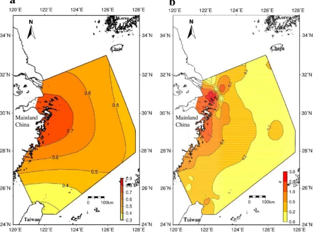
Figure6compares the GRACE-derived EWH rates (without land values) with the MARs from the sediment core measurements of Deng et al. [5]; see Section2.4for the numerical equivalence of MARs from GRACE and from sediment core measurements. Figure6shows that the EWH rates from GRACE are generally consistent with the sediment core-derived MARs in magnitude and spatial
Remote Sens. 2016, 8, 777 10 of 19
pattern, suggesting that GRACE is able to detect mass changes caused by the sediment deposition on the ECS inner shelf.
Remote Sens. 2016, 8, 777 10 of 19
spatial pattern, suggesting that GRACE is able to detect mass changes caused by the sediment deposition on the ECS inner shelf.
Figure 6. Sediment MARs (in cm/year) over April 2002–March 2015 from (a) GRACE and (b)
sediment core measurements [4]. The EWH rate is equivalent to MAR (see Section 3.1).
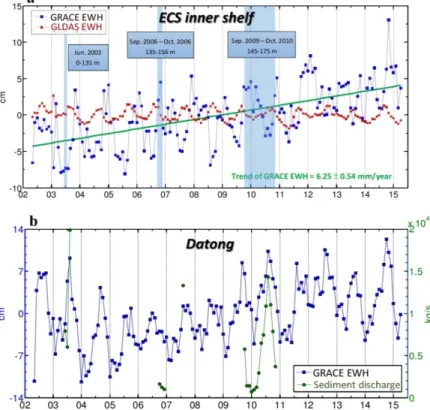
In order to show that the MAR signals in Figure 5 do not originate from errors in the GLDAS model, in Figure 7a, we compare the EWHs from GRACE (the mean of CSR, JPL and GFZ) and the EWHs from GLDAS (Section 2.3) on the ECS inner shelf. The GLDAS-derived EWHs (Section 2.3) are far smaller than the GRACE-derived EWHs, implying that the latter is not dominated by the former. Furthermore, Figure 7b compares the in situ sediment discharge of the Yangtze River at the Datong hydrographic station (see Figure 1) located at 30.10°N, 117.12°E and the GRACE-derived EWHs around this station (for convenience and because of GRACE’s limited spatial resolution, we use the EWHs at a grid point located at 30°N, 117°E). Note that the sediment discharge data at Datong are only partially available in 2003, 2006, 2007, 2009 and 2010, not the entire period of GRACE (April 2002–March 2015). The phase of the sediment discharge at Datong is the same as the phase of EWHs around Datong. In Figure 7b, both time series of GRACE-derived EWHs and in situ sediment discharge have peaks in the summer of 2010. A summer EWH peak on land is typical in the Northern Hemisphere because soil moistures and groundwater levels are usually high in summer [35]. In summary, the GRACE-derived EWH variations on the ECS inner shelf (Figure 4) are different from those on land (Figure 7b), particularly in the phase of annual oscillation, and are the result of sediment deposition on the ECS inner shelf. Dai and Lu showed that the TGD has reduced Yangtze’s sediment loads [7]. We postulate that the reduction in loads will lead to a reduced sediment deposition in the Yangtze estuary and consequently on the ECS inner shelf. Here, we examine whether GRACE can detect such reductions. In Figure 7a, we mark the time periods of the three impoundments of the TGD in 2003, 2006 and 2009–2010. From Figure 7a, it appears that the sediment deposition pattern from GRACE was not altered by the impoundments. In particular, the EWH was still rising after the last impoundment in late October 2010. From Figure 7b, again,
Figure 6.Sediment MARs (in cm/year) over April 2002–March 2015 from (a) GRACE and (b) sediment core measurements [4]. The EWH rate is equivalent to MAR (see Section3.1).
In order to show that the MAR signals in Figure5do not originate from errors in the GLDAS model, in Figure7a, we compare the EWHs from GRACE (the mean of CSR, JPL and GFZ) and the EWHs from GLDAS (Section2.3) on the ECS inner shelf. The GLDAS-derived EWHs (Section2.3) are far smaller than the GRACE-derived EWHs, implying that the latter is not dominated by the former. Furthermore, Figure7b compares the in situ sediment discharge of the Yangtze River at the Datong hydrographic station (see Figure1) located at 30.10◦N, 117.12◦E and the GRACE-derived EWHs around this station (for convenience and because of GRACE’s limited spatial resolution, we use the EWHs at a grid point located at 30◦N, 117◦E). Note that the sediment discharge data at Datong are only partially available in 2003, 2006, 2007, 2009 and 2010, not the entire period of GRACE (April 2002–March 2015). The phase of the sediment discharge at Datong is the same as the phase of EWHs around Datong. In Figure7b, both time series of GRACE-derived EWHs and in situ sediment discharge have peaks in the summer of 2010. A summer EWH peak on land is typical in the Northern Hemisphere because soil moistures and groundwater levels are usually high in summer [35]. In summary, the GRACE-derived EWH variations on the ECS inner shelf (Figure4) are different from those on land (Figure7b), particularly in the phase of annual oscillation, and are the result of sediment deposition on the ECS inner shelf. Dai and Lu showed that the TGD has reduced Yangtze’s sediment loads [7]. We postulate that the reduction in loads will lead to a reduced sediment deposition in the Yangtze estuary and consequently on the ECS inner shelf. Here, we examine whether GRACE can detect such reductions. In Figure7a, we mark the time periods of the three impoundments of the TGD in 2003, 2006 and 2009–2010. From Figure7a, it appears that the sediment deposition pattern from GRACE was not altered by the impoundments. In particular, the EWH was still rising after the last impoundment in late October 2010. From Figure7b,
again, there is no clear modulation of the EWH oscillations. A further investigation of the relationship between the TGD and EWH change is carried out in Section3.2using wavelet analysis.
Remote Sens. 2016, 8, 777 11 of 19
there is no clear modulation of the EWH oscillations. A further investigation of the relationship between the TGD and EWH change is carried out in Section 3.2 using wavelet analysis.
Figure 7. EWHs from GRACE and comparison with the sediment discharge of Yangtze. (a) EWHs
on the ECS inner shelf from mean GRACE products and GLDAS; (b) Comparison between measured sediment discharges of the Yangtze River at the Datong hydrographic station and GRACE-derived EWHs around this station. The shaded periods mark the time periods of impoundments of the Three Gorge Dam (TGD). In June 2003, the TGD water level was raised to 135 m above sea level, followed by the rise to 156 m in late October 2006 and, finally, to 175 m in late October 2010.
Using the mean EWHs over the dashed box in Figure 5, we determined the rate of mass change over April 2002–March 2015. The area of the dashed box is approximate 2.15 × 10⁵ km2. Table 2
shows the rates of mass change from three GRACE products and their mean value. The GRACE-derived rates of mass change range from 1.21–1.51 × 10⁹ ton/year, which are compatible in
magnitude with the value of 0.9–1.0 × 10⁹ ton/year given in Table 2 of Deng et al. [5]. There are at
least two factors contributing to the larger GRACE-derived MARs (this study) than the in situ measurements. First, the GRACE-derived MARs contain non-sediment signals, which were not completely removed by the models in Table 1. Second, we estimate MARs only over the dashed box in Figure 5 covering just a part of the ECS inner shelf, but Deng et al. estimated MARs over the entire ECS using higher mass accumulations in east China’s offshore areas and lower mass accumulations in the deeper waters of the ECS [5].
Table 2. GRACE-derived rate of EWH and the inferred rate of mass change over
April 2002–March 2015 (156 months) in the dashed box defined in Figure 5 (note: one m3 of water
corresponds to one ton).
CSR JPL GFZ Mean
Rate of EWH (mm/year) 6.09 7.04 5.61 6.25
Rate of mass change (×109 ton/year) 1.31 1.51 1.21 1.34
Figure 7.EWHs from GRACE and comparison with the sediment discharge of Yangtze. (a) EWHs on the ECS inner shelf from mean GRACE products and GLDAS; (b) Comparison between measured sediment discharges of the Yangtze River at the Datong hydrographic station and GRACE-derived EWHs around this station. The shaded periods mark the time periods of impoundments of the Three Gorge Dam (TGD). In June 2003, the TGD water level was raised to 135 m above sea level, followed by the rise to 156 m in late October 2006 and, finally, to 175 m in late October 2010.
Using the mean EWHs over the dashed box in Figure5, we determined the rate of mass change over April 2002–March 2015. The area of the dashed box is approximate 2.15×10⁵km2. Table2shows the rates of mass change from three GRACE products and their mean value. The GRACE-derived rates of mass change range from 1.21–1.51×10⁹ton/year, which are compatible in magnitude with the value of 0.9–1.0×10⁹ton/year given in Table2of Deng et al. [5]. There are at least two factors contributing to the larger GRACE-derived MARs (this study) than the in situ measurements. First, the GRACE-derived MARs contain non-sediment signals, which were not completely removed by the models in Table1. Second, we estimate MARs only over the dashed box in Figure5covering just a part of the ECS inner shelf, but Deng et al. estimated MARs over the entire ECS using higher mass accumulations in east China’s offshore areas and lower mass accumulations in the deeper waters of the ECS [5].
Table 2.GRACE-derived rate of EWH and the inferred rate of mass change over April 2002–March 2015 (156 months) in the dashed box defined in Figure5(note: one m3of water corresponds to one ton).
CSR JPL GFZ Mean
Rate of EWH (mm/year) 6.09 7.04 5.61 6.25
Remote Sens. 2016, 8, 777 12 of 19
3.2. Variability of Sediment Mass in the ECS: From Semi-Annual to Inter-Annual Oscillations
Unlike time-lapse sediment core measurements that can only yield rates of mass accumulation, GRACE can deliver continuous records at a regular time interval, such as those given in Figure7a. As such, GRACE is able to show the variability of sediment mass accumulation at varying time scales. To identify the components of the variability, we carried out a wavelet analysis of the GRACE-derived EWHs. Figure8a,b show the detrended time series of EWHs (based on that in Figure7a) and its wavelet spectrum. In practice, we used the MATLAB continuous wavelet tool “CWT” to compute the wavelet coefficients with the Morlet function as the basis function. A wavelet coefficient is similar to a wavelet power spectrum. Because of the normalization, the wavelet coefficients in Figure8are unitless. Coefficients of 10 and−10 indicate maximum positive and negative correlations between a signal component (oscillation) and a wavelet basis function at a specific time scale. A coefficient of zero indicates the least similarity between a signal component and a basis function. In addition, to link the oscillations of EWHs to El Niño-Southern Oscillation (ENSO), we obtained the time series of the Multivariate ENSO Index (MEI; Figure8c) from NOAA [36] and computed its wavelet spectrum (Figure8d). The following interpretation of the time variation of amplitude and occurrence frequency of a given oscillation is based on Torrence and Compo (1998) [37], with the possible cause of the oscillation presented.
Remote Sens. 2016, 8, 777 12 of 19
3.2. Variability of Sediment Mass in the ECS: From Semi-Annual to Inter-Annual Oscillations
Unlike time-lapse sediment core measurements that can only yield rates of mass accumulation, GRACE can deliver continuous records at a regular time interval, such as those given in Figure 7a. As such, GRACE is able to show the variability of sediment mass accumulation at varying time scales. To identify the components of the variability, we carried out a wavelet analysis of the GRACE-derived EWHs. Figure 8a,b show the detrended time series of EWHs (based on that in Figure 7a) and its wavelet spectrum. In practice, we used the MATLAB continuous wavelet tool “CWT” to compute the wavelet coefficients with the Morlet function as the basis function. A wavelet coefficient is similar to a wavelet power spectrum. Because of the normalization, the wavelet coefficients in Figure 8 are unitless. Coefficients of 10 and −10 indicate maximum positive and negative correlations between a signal component (oscillation) and a wavelet basis function at a specific time scale. A coefficient of zero indicates the least similarity between a signal component and a basis function. In addition, to link the oscillations of EWHs to El Niño-Southern Oscillation (ENSO), we obtained the time series of the Multivariate ENSO Index (MEI; Figure 8c) from NOAA [36] and computed its wavelet spectrum (Figure 8d). The following interpretation of the time variation of amplitude and occurrence frequency of a given oscillation is based on Torrence and Compo (1998) [37], with the possible cause of the oscillation presented.
Figure 8. (a) Time series of detrended GRACE-derived EWHs and (b) their wavelet spectrum; (c)
Time series of the Multivariate ENSO Index (MEI) obtained from NOAA [36] and (d) its wavelet spectrum.
Figure 8.(a) Time series of detrended GRACE-derived EWHs and (b) their wavelet spectrum; (c) Time series of the Multivariate ENSO Index (MEI) obtained from NOAA [36] and (d) its wavelet spectrum.
3.3. Semi-Annual Oscillation (the Period Is Six Months)
This oscillation corresponds to local highs in spring and fall and local lows in summer and winter, especially in 2003, and from 2006–2011. These highs and lows are largely due to the seasonal reversals of East Asian monsoon winds: the summer monsoon carries moist airs from the tropical oceans to East Asia [38], while the winter monsoon carries dry airs from Siberia to East Asia [39]. Such varying air moisture contents modify rains and erosion in the Yangtze basin, thereby modulating the pattern of sediment deposition on the ECS inner shelf at the semi-annual time scale. Figure8b shows that the semi-annual oscillations are particularly strong during 2006–2008 and from 2014 onward.
3.4. Annual Oscillation (the Period Is 12 Months)
This oscillation is evident throughout the entire GRACE records from April 2002–March 2015. On the ECS inner shelf, the GRACE-derived sediment deposition is high in winter and low in summer. This annual high-low pattern is consistent with those from in situ measurements [6,40] and from model predictions [41]. The annual oscillation can be qualitatively explained by the ocean circulation pattern associated with the sediment dispersal path in the ECS. As shown in Figure1, the ECSCC includes the Jiangsu Coastal Current (JCC) in the north and the Zhejiang Fujian Coastal Current (ZFCC) in the south [8], and it flows southward in fall and winter while flowing northward in summer [42,43]. The TWC and the KC are in the west and east of the ECS, respectively, and both are strong in summer and weak in winter. In fall and winter, the southward-flowing ECSCC is gradually intensified by the northeast monsoon and interacts with the weaker northward-flowing TWC. As such, most of the sediments are trapped on the ECS inner shelf [40]. In summer, the northward-flowing ECSCC and TWC combine to cause less sediment deposition on the ECS inner shelf. Such an interaction between the ECSCC and the TWC results in the seasonal cycle of sediment deposition consistent with the MAR signals detected by GRACE, as seen in Figure8a (time series) and Figure8b (the concentrated wavelet power spectrum at the one-year period).
Here, we present two more factors that can affect the annual oscillation of the ECS sediment deposition. First, as the East Asian winter monsoon intensifies, higher waves in the Yangtze estuary are generated and induce more energetic flows in the Yangtze estuary in winter [44]. Under the physical deposition effect, more energetic hydrodynamics results in coarser sediments. This implies that relatively coarser sediments tend to deposit in winter, while finer ones prevail in depositing in summer [42]. In contrast to the coarser sediments in winter, the finer sediments in summer may be easily transported by coastal currents and thus have a short residence time. Second, in winter, the Changjiang plume is constrained by an enhanced ECSCC to flow southward in a narrow band to deposit sediments along the coast of China. In summer, the Changjiang plume is dispersed toward the north and the east [45], resulting in less sediment deposition in Yangtze’ offshore regions.
3.5. Quasi-Biennial Oscillation (the Period Is about Two Years)
This oscillation has a period of about two years and is named the quasi-biennial oscillation. This oscillation is evident in the wavelet spectrum of EWH (Figure8b), but its magnitude is smaller than the magnitudes of the semi-annual and annual oscillations. In addition, the wavelet spectrum of MEI (Figure8d) also contains the quasi-biennial oscillation, despite its lower magnitude compared to other oscillations. Lindzen et al. showed a quasi-biennial oscillation in atmospheric circulation that causes a precipitation oscillation of the same period [46]. Such a quasi-biennial precipitation oscillation in the Yangtze basin introduces variations in soil erosion, subsequently affecting the variations of sediment deposition at a nearly two-year interval in the ECS. The quasi-biennial oscillation in soil erosion also leads to vertical surface deformations at a similar period that are detected by continuous GPS records in the Yangtze basin [47]. The quasi-biennial high in 2009–2010 is exceptionally large, and the quasi-biennial lows in 2008–2009 and 2010–2011 have anomalous magnitudes (Figure8b). These extreme values coincide with the oscillations of ENSO during 2008–2011 (Figure8d).
Remote Sens. 2016, 8, 777 14 of 19
3.6. Interannual Oscillation
In addition to the quasi-biennial oscillation, Figure8b also shows evident oscillations at periods of three and five years. The three-year oscillation is also clear in the wavelet spectrum of ENSO, with a less obvious five-year oscillation. However, during the strong three-year ENSO oscillation between 2008 and 2011, the magnitude of the three-year oscillation of EWH decreases, but the magnitude of the quasi-biennial oscillation increases. Such modulations of the amplitudes of the two- and three-year oscillations may be the result of the interaction between the oscillations of various periods. In Figure8c, the interannual highs from late 2009–early 2010 may be associated with an El Niño that has caused a record-breaking warm sea surface temperature anomaly in the central Pacific Ocean. This 2009–2010 El Niño later underwent a fast phase transition to La Niña [48], which caused a 5-mm drop in global mean sea level [49]. In addition, with a phase lag, the large quasi-biennial low of EWH in 2008–2009 (Figure8b) seems to be correlated with the 2007–2008 La Niña, which caused a severe drought in the northern Yangtze valley [50] that substantially reduced Yangtze’ sediment yield and potentially reduced the sediment deposition on the ECS inner shelf. In the four sub-figures of Figure8, we highlight these connections by pointers and annotations.
Figure8b shows that the annual pattern is changed after 2010. Three notable changes are: (1) the intensified winter high in the 2011–2012 winter; (2) the weakened, prolonged winter high in the 2012–2013 winter; and (3) almost the disappearance of the winter high in the 2013–2014 winter. It is not clear that this pattern change is linked to the completion of the TGD in October 2010 or is the result of the interaction between the annual oscillation and the interannual oscillation in the ocean and atmosphere that lead to the pattern change in erosion and, subsequently, in sediment. Because the time period from October 2010 to the present (June 2016) is short, the result reported here about the impact of TGD on the ECS sediment deposition is inconclusive.
3.7. Decadal Oscillation
There is a potential decadal oscillation linked to the Pacific Decadal Oscillation (PDO) [51]. However, the current GRACE record is too short to adequately show the decadal oscillation. The GRACE Follow-on, a successor to the GRACE mission, which is scheduled for launch in 2017, may provide an extended time series to detect this oscillation.
4. Discussion: Can We Detect MARS by GRACE in the World’s Major Estuaries?
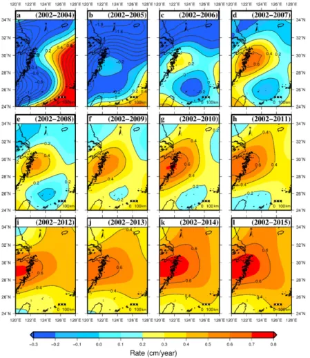
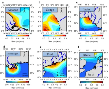
In Section3, we have shown clear MAR signals from GRACE on the ECS inner shelf. A question arises as to whether we can use GRACE to detect MAR signals in the estuaries of the world’s major rivers, such as the Amazon, Congo, Indus, Mississippi, Pear and Rhine River. The answer depends on at least two factors: (1) uncertainties in the GRACE-derived MARs; and (2) the interaction between ocean circulations and the oceanic environment around a river estuary. First, the uncertainty of GRACE-derived mass-related signals around river estuaries is governed by GRACE’s data quality, spatial resolution and the uncertainties of the models for removing the non-sediment-induced gravity effects. To illustrate the effect of the uncertainties, in Figure9, we show GRACE-derived EWH rates in the ECS spanning different time periods. The spatial patterns of EWH rates vary over different periods. In general, the patterns of EWH rates from short-term GRACE observations (less than four years; Figure9a–c) are not consistent with that from sediment-core measurements (Figure6b). A reliable spatial pattern of sediment deposition begins to form when using GRACE records over 2002–2007 (Figure9d). That is, GRACE records must be sufficiently long to generate a favourable signal to noise ratio. To address partially the second factor, Figure10shows the GRACE-derived EWH rates in six selected estuaries in the world where we attempted to find potential MAR signals. The spatial patterns of EWH over the six estuaries in Figure10are different. Whether the MAR signals in Figure10are true or artefacts requires verifications using ground-based data, such as those presented in Figure6b for the ECS.
Again, we emphasize the importance of the interaction between ocean currents and estuaries in the formation of sediment deposition. As stated in Sections1and3.2, the interaction of the ocean currents near the Yangtze estuary (Figure1) forms the right conditions for sediments to deposit on the ESC inner shelf. Here, we show two more examples to briefly explain how sediment depositions around a river estuary can be influenced by ocean tides, ocean currents and ocean bottom topography. First, the Pearl River estuary is predominated by ebb flows (about 2 m/s) that have strong speeds and long durations [52]. The ebb flows trap sediments transported by the Pearl River, allowing sediments to form around its estuary and resulting in the potential MAR signal seen in Figure10e. Second, around the Congo estuary, the Congo Canyon immediately off Congo’s west coast serves as a conduit for turbidity currents to carry away sediments from the Congo River to the oceans [53]. In addition, the branch of the northward flowing Benguela Current along the west coast of Africa can reduce sediment depositions on the northern side of the Congo River estuary [54], which may cause the potential MAR signal to emerge north of Congo’s estuary in Figure10b. Again, the GRACE data quality is another deciding factor: it is likely that GRACE data uncertainties in some of the estuaries in Figure10 are so overwhelming that they suppress potential MAR signals. If this is the case, then perhaps future GRACE releases could reduce such data uncertainties, allowing sediment MAR signals to emerge. Finally, filtering and leakage can also lead to losses of MAR signals. Interested readers are encouraged to improve their GRACE data processing techniques and to study the condition of estuary-ocean circulation for detecting sediment deposition around an estuary that is sufficiently large in MAR signal and in GRACE’s spatial resolution. A comprehensive guide for searching MAR signals around estuaries is the book by Millian and Farnsworth [55].
Electronics 2016, 5, x FOR PEER REVIEW 4 of 4
Today, the great calculus capability of the digital systems, allows developing instruments able to limit the effects of the deviations [17]. To evaluate the PQ [18], it is necessary to make measurements. Over the years, we realized and perfected a probe able to determine in real time the quality parameters with a high confidence level and we developed an ad hoc instrument to satisfy some characteristics that is usually difficult to find in one instrument available in the market.
Figure 9.(a–l) Different spatial patterns of EWH rates on the ECS inner shelf using GRACE records spanning different time periods.
Remote Sens. 2016, 8, 777 16 of 19
Remote Sens. 2016, 8, 777 16 of 19
Figure 10. GRACE-derived EWH rates near the estuaries of the (a) Amazon; (b) Congo; (c) Indus;
(d) Mississippi; (e) Pearl and (f) Rhine rivers over April 2002–March 2015. 5. Conclusions
In this paper, we show a new application of GRACE: detecting sediment deposition on the ECS inner shelf. The ECS has an ideal shallow-water ocean circulation system that allows depositing sufficiently large offshore sediments that can be detected by GRACE. A successful detection requires a proper data processing of the GRACE products and use of auxiliary data (such as GLDAS). The favourable result is based on the GSM SHCs restored with the SHCs of atmospheric and oceanic effects (GAD). Restoring GAD can avoid contaminations of sediment signals caused by the errors in the models for GAD. We also applied a decorrelation filter to reduce the stripes and a 250-km Gaussian filter to reduce high-frequency noises. The leakage effect near the coastal regions of the ECS inner shelf was reduced using the hydrological model GLDAS.
On the ECS inner shelf, the GRACE-derived EWHs reflect mass anomalies associated with sediment deposition. The mass changes due to changes in ocean bottom pressure and land hydrology are too small to be the dominating contributors to the GRACE-derived EWHs. The mean rates of GRACE-derived EWHs on the ECS inner shelf from the three GRACE products are quite consistent and are about 6 mm/year. The GRACE-derived sediment MARs are consistent with those from in situ measurements using sediment cores. The GRACE-derived EWHs also show oscillations of sediment deposition on the ECS inner shelf at semi-annual to inter-annual time scales, which reflect the varying erosions caused by varying rains associated with East Asia monsoons and ENSO events and by seasonal varying oceanic circulations around the ECS. Such oscillations can only be possibly measured by a mission like GRACE that can continuously deliver long-term monthly mass variations, which will be continued by its follow-on mission for possibly another decade. A monthly in situ survey of sediment cores over an area like the ECS will be too costly and time-consuming. However, sediment-core measurements are imperative to assess and constrain the rates of sediment deposition from GRACE. To encourage the use of GRACE in detecting offshore sediment deposition, we show the potential MAR signals in six selected estuaries. MAR signals in some of the estuaries are clear, while some are obscure. The current limitation of GRACE in detecting offshore sediment deposition is its low (about 250 km) spatial resolution and possible contaminations by land hydrological and oceanic signals. GRACE could detect potential MAR signals in estuaries other than the Yangtze estuary, but further studies are needed to substantiate the result.
Figure 10. GRACE-derived EWH rates near the estuaries of the (a) Amazon; (b) Congo; (c) Indus; (d) Mississippi; (e) Pearl and (f) Rhine rivers over April 2002–March 2015.
5. Conclusions
In this paper, we show a new application of GRACE: detecting sediment deposition on the ECS inner shelf. The ECS has an ideal shallow-water ocean circulation system that allows depositing sufficiently large offshore sediments that can be detected by GRACE. A successful detection requires a proper data processing of the GRACE products and use of auxiliary data (such as GLDAS). The favourable result is based on the GSM SHCs restored with the SHCs of atmospheric and oceanic effects (GAD). Restoring GAD can avoid contaminations of sediment signals caused by the errors in the models for GAD. We also applied a decorrelation filter to reduce the stripes and a 250-km Gaussian filter to reduce high-frequency noises. The leakage effect near the coastal regions of the ECS inner shelf was reduced using the hydrological model GLDAS.
On the ECS inner shelf, the GRACE-derived EWHs reflect mass anomalies associated with sediment deposition. The mass changes due to changes in ocean bottom pressure and land hydrology are too small to be the dominating contributors to the GRACE-derived EWHs. The mean rates of GRACE-derived EWHs on the ECS inner shelf from the three GRACE products are quite consistent and are about 6 mm/year. The GRACE-derived sediment MARs are consistent with those from in situ measurements using sediment cores. The GRACE-derived EWHs also show oscillations of sediment deposition on the ECS inner shelf at semi-annual to inter-annual time scales, which reflect the varying erosions caused by varying rains associated with East Asia monsoons and ENSO events and by seasonal varying oceanic circulations around the ECS. Such oscillations can only be possibly measured by a mission like GRACE that can continuously deliver long-term monthly mass variations, which will be continued by its follow-on mission for possibly another decade. A monthly in situ survey of sediment cores over an area like the ECS will be too costly and time-consuming. However, sediment-core measurements are imperative to assess and constrain the rates of sediment deposition from GRACE. To encourage the use of GRACE in detecting offshore sediment deposition, we show the potential MAR signals in six selected estuaries. MAR signals in some of the estuaries are clear, while some are obscure. The current limitation of GRACE in detecting offshore sediment deposition is its low (about 250 km) spatial resolution and possible contaminations by land hydrological and oceanic signals. GRACE could detect potential MAR signals in estuaries other than the Yangtze estuary, but further studies are needed to substantiate the result.
Acknowledgments: This study is supported by the Ministry of Science and Technology (MOST), Taiwan, under Grants 103-2221-E-009-114-MY3 and 104-2611-M-009-001. This paper is dedicated to the memory of Chih-An Huh (1952–2015), Institute of Earth Sciences, Academia Sinica, who assisted the authors in the early stage of this study. We thank Jinhai Zheng of Hohai University, China, for providing the sediment discharge measurements of the Yangtze River at Datong station (Figure1). We thank the reviewers for their constructive comments.
Author Contributions:C.H. initiated the idea in this study. Y.C.L. performed most of the data analysis. Y.C.L. and C.H. wrote the first draft. J.H., R.K., C.R.W., H.C.S. and N.T. assisted Y.C.L. and C.H. with data analysis and interpretation. All authors read and approved the final draft.
Conflicts of Interest:The authors declare that they have no competing interests. References
1. Chen, X.; Zong, Y.; Zhang, E.; Xu, J.; Li, S. Human impacts on the Changjiang (Yangtze) River Basin, China, with special reference to the impacts on the dry season water discharges into the sea. Geomorphology 2001, 41, 111–123. [CrossRef]
2. Holeman, J.N. The sediment yield of major rivers of the world. Water Resour. Res. 1968, 4, 737–747. [CrossRef] 3. Xian, Q.; Ramu, K.; Isobe, T.; Sudaryanto, A.; Liu, X.; Gao, Z.; Takahashi, S.; Yu, H.; Tanabe, S. Levels and body distribution of polybrominated diphenyl ethers (PBDEs) and hexabromocyclododecanes (HBCDs) in freshwater fishes from the Yangtze River, China. Chemosphere 2008, 71, 268–276. [CrossRef] [PubMed] 4. Milliman, J.D.; Meade, R.H. World-wide delivery of river sediment to the oceans. J. Geol. 1983, 91, 1–21.
[CrossRef]
5. Deng, B.; Zhang, J.; Wu, Y. Recent sediment accumulation and carbon burial in the East China Sea. Glob. Biogeochem. Cycles 2006. [CrossRef]
6. Xu, K.; Milliman, J.D.; Li, A.; Paul Liu, J.; Kao, S.J.; Wan, S. Yangtze- and Taiwan-derived sediments on the inner shelf of East China Sea. Cont. Shelf Res. 2009, 29, 2240–2256. [CrossRef]
7. Dai, S.B.; Lu, X.X. Sediment load change in the Yangtze River (Changjiang): A review. Geomorphology 2014, 215, 60–73. [CrossRef]
8. Liu, J.P.; Li, A.C.; Xu, K.H.; Velozzi, D.M.; Yang, Z.S.; Milliman, J.D.; DeMaster, D.J. Sedimentary features of the Yangtze River-derived along-shelf clinoform deposit in the East China Sea. Cont. Shelf Res. 2006, 26, 2141–2156. [CrossRef]
9. Su, C.C.; Huh, C.A.210Pb,137Cs and239, 240Pu in East China Sea sediments: Sources, pathways and budgets of sediments and radionuclides. Mar. Geol. 2002, 183, 163–178. [CrossRef]
10. Huh, C.A.; Su, C.C. Sedimentation dynamics in the East China Sea elucidated from210Pb,137Cs and239, 240Pu. Mar. Geol. 1999, 160, 183–196. [CrossRef]
11. Tapley, B.D.; Bettadpur, S.; Ries, J.C.; Thompson, P.F.; Watkins, M.M. GRACE measurements of mass variability in the Earth system. Science 2004, 305, 503–505. [CrossRef] [PubMed]
12. Velicogna, I.; Wahr, J. Greenland mass balance from GRACE. Geophys. Res. Lett. 2005, 32, L18505. [CrossRef] 13. Velicogna, I.; Wahr, J. Measurements of time-variable gravity show mass loss in Antarctica. Science 2006, 311,
1754–1756. [CrossRef] [PubMed]
14. Rodell, M.; Velicogna, I.; Famiglietti, J.S. Satellite-based estimates of groundwater depletion in India. Nature
2009, 460, 999–1002. [CrossRef] [PubMed]
15. Feng, W.; Zhong, M.; Lemoine, J.-M.; Biancale, R.; Hsu, H.T.; Xia, J. Evaluation of groundwater depletion in North China using the Gravity Recovery and Climate Experiment (GRACE) data and ground-based measurements. Water Resour. Res. 2013, 49, 2110–2118. [CrossRef]
16. Chambers, D.P.; Bonin, J.A. Evaluation of Release-05 GRACE time-variable gravity coefficients over the ocean. Ocean Sci. 2012, 8, 859–868. [CrossRef]
17. Tregoning, P.; Lambeck, K.; Ramillien, G. GRACE estimates of sea surface height anomalies in the Gulf of Carpentaria, Australia. Earth Planet. Sci. Lett. 2008, 271, 241–244. [CrossRef]
18. Wouters, B.; Chambers, D. Analysis of seasonal ocean bottom pressure variability in the Gulf of Thailand from GRACE. Glob. Planet. Chang. 2010, 74, 76–81. [CrossRef]
19. Feng, W.; Lemoine, J.M.; Zhong, M.; Hsu, H.T. Mass-induced sea level variations in the Red Sea from GRACE, steric-corrected altimetry, in situ bottom pressure records, and hydrographic observations. J. Geodyn. 2014, 78, 1–7. [CrossRef]
Remote Sens. 2016, 8, 777 18 of 19
20. Bettadpur, S. Level-2 Gravity Field Product User Handbook. Available online: ftp://podaac.jpl.nasa.gov/ allData/grace/docs/L2-UserHandbook_v3.0.pdf (accessed on 26 May 2016).
21. Flechtner, F.; Dobslaw, H.; Fagiolini, E. AOD1B Product Description Document for Product Release 05 (Rev. 4.4). Available online: ftp://podaac.jpl.nasa.gov/allData/grace/docs/AOD1B_PDD_v4.4.pdf (accessed on 24 March 2016).
22. Chen, J.L.; Rodell, M.; Wilson, C.R.; Famiglietti, J.S. Low degree spherical harmonic influences on Gravity Recovery and Climate Experiment (GRACE) water storage estimates. Geophys. Res. Lett. 2005. [CrossRef] 23. Swenson, S.; Chambers, D.; Wahr, J. Estimating geocenter variations from a combination of GRACE and
ocean model output. J. Geophys. Res. 2008. [CrossRef]
24. Cheng, M.; Ries, J.C.; Tapley, B.D. Variations of the Earth’s figure axis from satellite laser ranging and GRACE. J. Geophys. Res. 2011, 116, B01409. [CrossRef]
25. Swenson, S.; Wahr, J. Post-processing removal of correlated errors in GRACE data. Geophys. Res. Lett. 2006. [CrossRef]
26. Tangdamrongsub, N.; Hwang, C.; Shum, C.K.; Wang, L. Regional surface mass anomalies from GRACE KBR measurements: Application of L-curve regularization and a priori hydrological knowledge. J. Geophys. Res.
2012. [CrossRef]
27. Wahr, J.; Molenaar, M.; Bryan, F. Time variability of the Earth’s gravity field: Hydrological and oceanic effects and their possible detection using GRACE. J. Geophys. Res. 1998, 103, 30205–30229. [CrossRef]
28. Guo, J.Y.; Duan, X.J.; Shum, C.K. Non-isotropic Gaussian smoothing and leakage reduction for determining mass changes over land and ocean using GRACE data. Geophys. J. Int. 2010, 181, 290–302. [CrossRef] 29. Bonin, J.; Chambers, D. Uncertainty estimates of a GRACE inversion modelling technique over Greenland
using a simulation. Geophys. J. Int. 2013, 194, 212–229. [CrossRef]
30. Tangdamrongsub, N.; Hwang, C.; Kao, Y.C. Water storage loss in central and South Asia from GRACE satellite gravity: Correlations with climate data. Nat. Hazards 2011, 59, 749–769. [CrossRef]
31. Rodell, M.; Houser, P.R.; Jambor, U.; Gottschalck, J.; Mitchell, K.; Meng, C.J.; Arsenault, K.; Cosgrove, B.; Radakovich, J.; Bosilovich, M.; et al. The global land data assimilation system. Bull. Am. Meteorol. Soc. 2004, 85, 381–394. [CrossRef]
32. Hwang, C.; Kao, Y.C. Spherical harmonic analysis and synthesis using FFT: Application to temporal gravity variation. Comput. Geosci. 2006, 32, 442–451. [CrossRef]
33. Yi, S.; Wang, Q.; Sun, W. Basin mass dynamic changes in China from GRACE based on a multibasin inversion method. J. Geophys. Res. Solid Earth. 2016. [CrossRef]
34. Sakumura, C.; Bettadpur, S.; Bruinsma, S. Ensemble prediction and intercomparison analysis of GRACE time-variable gravity field models. Geophys. Res. Lett. 2014, 41, 1389–1397. [CrossRef]
35. Trenberth, K.E.; Smith, L.; Qian, T.; Dai, A.; Fasullo, J. Estimates of the global water budget and its annual cycle using observational and model data. J. Hydrometeorol. 2007, 8, 758–769. [CrossRef]
36. NOAA Earth System Research Laboratory. Available online: http://www.esrl.noaa.gov/psd/enso/mei/ table.html (accessed on 29 May 2016).
37. Torrence, C.; Compo, G.P. A Practical Guide to Wavelet Analysis. Bull. Am. Meteorol. Soc. 1998, 79, 61–78. [CrossRef]
38. Ding, Y.; Chan, J.C.L. The East Asian summer monsoon: An overview. Meteorol. Atmos. Phys. 2005, 89, 117–142.
39. Chang, C.P.; Wang, Z.; Hendon, H. The Asian winter monsoon. In The Asian Monsoon; Wang, B., Ed.; Praxis Publishing Ltd.: Chichester, UK, 2006; pp. 89–127.
40. Liu, J.P.; Xu, K.H.; Li, A.C.; Milliman, J.D.; Velozzi, D.M.; Xiao, S.B.; Yang, Z.S. Flux and fate of Yangtze River sediment delivered to the East China Sea. Geomorphology 2007, 85, 208–224. [CrossRef]
41. Zeng, X.; He, R.; Xue, Z.; Wang, H.; Wang, Y.; Yao, Z.; Guan, W.; Warrillow, J. River-derived sediment suspension and transport in the Bohai, Yellow, and East China Seas: A preliminary modeling study. Cont. Shelf Res. 2015, 111, 112–125. [CrossRef]
42. Xiao, S.; Li, A.; Liu, J.P.; Chen, M.; Xie, Q.; Jiang, F.; Li, T.; Xiang, R.; Chen, Z. Coherence between solar activity and the East Asian winter monsoon variability in the past 8000 years from Yangtze River-derived mud in the East China Sea. Palaeogeogr. Palaeoclimatol. Palaeoecol. 2006, 237, 293–304. [CrossRef]
43. Su, J.L. A review of circulation dynamics of the coastal oceans near China. Acta Oceanol. Sin. 2001, 23, 1–16. (In Chinese)