使用外匯隱含波動率建構利差交易策略-馬可夫轉換模型之應用 - 政大學術集成

全文

(1)國立政治大學金融學系碩士班碩士論文 Department of Money and Banking National Cheng-Chi University Master Thesis. 使用外匯隱含波動率建構利差交易策略-馬可夫轉換治. 立. 政. 模型之應用. 大. ‧ 國. 學. Carry trade strategies in FX market by use of FX. ‧. implied volatility as an indicator. Nat. er. io. sit. y. - Application of Markov switching model. al. n. iv n C h e n g c h i U博士指導教授：陳威光林靖庭博士研究生：張誠文. 中華民國 103 年 6 月 1.

(2) 感謝詞兩年光陰轉瞬而逝，想當年升碩一時還懵懂無知，但在修過威光老師的選擇權之後，對選擇權及衍生性商品的高度興趣，便決定找威光老師當指導教授，老師也很重視指導學生，在碩一時便要我們去旁聽碩二的學長姐報論文，提前了解碩二生活的輪廓。碩二的生活相當緊湊，除了學校課業外，也希望增進財務知識，故同時準備 FRM 及 CFA 的證照考試，為了兼顧課業、論文及證照考試，在去年 9 月就決定以利差交易為題，並督促自己每天就算在疲累，也至少寫兩小時的論文，以維持論. 政治大化，碩二下壓力大到腸胃不適，晚上也常常驚醒，能一覺到天亮已是奢侈。立. 文進度及讓思緒連貫，即使已提前規劃未來一年的行程表，但計畫總是趕不上變. ‧ 國. 學. 論文能順利完成，首先感謝父母在這段期間的鼓勵，並支持我做的每一件決定。也感謝老姊，每天和我聊天，陪我度過這段艱辛的過程。也感謝威光及靖庭. ‧. 老師，每兩個禮拜的 meeting，給予我論文上的建議，威光老師除了學術上的建. sit. y. Nat. 議，也不時會找業界的學長姐回來分享，讓我們能提前了解理論與實務上的差異，. n. al. er. io. 靖庭老師也在我準備 CFA 考試時，提供許多寶貴意見，能找到兩位老師當指導教. i Un. v. 授，真的很開心，也很榮幸。同時感謝口試委員婁天威教授、郭維裕教授及徐政. Ch. engchi. 義教授，給予論文上的改進，讓本篇論文能更嚴謹。. 也謝謝在銀行交易室的阿湯學長(Alex Tang)，分享利差交易的實務經驗，讓這篇論文能更貼近實務的運作。遇到程式問題時，感謝黃柏崴的幫忙，節省不少摸索時間。也謝謝盧雲幫忙順英文論文稿，讓論文讀起來更流暢。也感謝陳英翰，擔起 meeting 團隊隊長的角色，論文進度之快令我們產生危機意識，也讓我們的論文能如期完稿。. 2.

(3) 摘要本文的目的是希望建構利差交易策略，以極大化策略的夏普比率為目標，本文以外匯隱含波動率當作訊號指標建立，利差交易策略，以期望其績效表現能勝過績效指標。本篇論文主要發現如下。第一，本文使用 8 種貨幣來檢驗無拋補利率平價假說 uncovered interest rate parity (UIP)，發現無拋補利率平價假說在所有貨幣中均不成立。第二，本文發現利率差可有效預測利差交易的報酬率，且利率差的係數隨著時間的推移而有遞減的現象。第三，本文使用馬可夫轉換模型把外. 政治大期外匯變動率的關係，本文發現，低利率貨幣在高波動度狀態下傾向升值，且外立匯市場分為低波動度及高波動度兩種狀態，並探討利率差、外匯隱含波動率及即. ‧ 國. 學. 匯隱含波動率是個不錯的指標，能用來判斷何時該平倉利差交易部位。最後，本文建立三個利差交易策略，分別為「持有到到期策略」、「外匯隱含. ‧. 波動率策略」及「組合式策略」，並把三種策略應用在澳元、紐元、墨西哥披索. sit. y. Nat. 及巴西里爾四種貨幣上，以評估不同策略的績效表現。本文發現「外匯隱含波動. n. al. er. io. 率策略」在樣本內及樣本外期間，均能賺取穩定的報酬率，「組合式策略」的績. i Un. v. 效有時能擊敗「外匯隱含波動率策略」，但有時其績效大幅落後「外匯隱含波動. Ch. 率策略」及「持有到到期策略」。. engchi. 本文建議，若機構投資人的風險容忍度為一般水準，可以實施「外匯隱含波動率策略」以賺取穩定報酬；若機構投資人有較高的風險容忍度，則可使用「組合式策略」，以賺取較高的預期報酬率。. 3.

(4) ABSTRACT The purpose of this paper is to build carry trade strategies and maximize the Sharpe ratio. This paper uses FX implied volatility as an indicator to build carry trade strategies and tries to outperform performance benchmark. Main findings in our paper are as follows. First, this paper tests the uncovered interest rate parity (UIP) and finds that UIP doesn’t hold in eight currencies over different investment periods. Second, interest rate differentials can predict the return of carry trade and the coefficients of interest rate differentials tend to decrease over time (five out of eight currencies). Third, this paper uses two-stage Markov-switching. 治政 model and divides the FX markets into high-volatility 大 and low-volatility state to 立 analysis the relationship between interest rate differentials, FX implied volatility and ‧ 國. 學. FX change. this paper finds that low-interest-rate currencies tend to appreciate in. ‧. high-volatility state. This paper also finds that FX implied volatility is a useful. sit. y. Nat. indicator to predict FX change and can be used to determine the timing to close out. io. er. carry trade positions.. al. Finally, this paper creates three carry trade strategies (buy-and-hold strategy, FX. n. iv n C implied volatility strategy, and combination to examine their performances h e n g cstrategy) hi U in four currencies. This paper finds that FX implied volatility strategy generates stable returns in both in-sample and out-of-sample period. Combination strategy sometimes could outperform FX implied volatility strategy. It’s appropriate for institutions with average risk tolerance to implement carry trade using FX implied volatility strategy. For institutions with above-average risk tolerance could implement Combination strategy to earn potentially higher returns.. 4.

(5) Contents. 1. Introduction & Motivations ....................................................................................... 9 2. Literature Reviews ................................................................................................... 12 2.1 Uncovered interest rate parity (UIP) .......................................................... 12 2.1.1 Literatures against UIP theory .......................................................... 13 2.1.2 Literatures support UIP theory.......................................................... 14 2.2 Carry trade ................................................................................................. 16. 政治大. 2.3 Markov switching model ......................................................................... 20. 立. ‧ 國. 學. 3. Methodology ............................................................................................................ 20 3.1 The forward premium anomalies ............................................................... 20. ‧. 3.2 Interest rate differential predicts returns of carry trade ............................. 22. sit. y. Nat. 3.3 Using OLS to find influential factors ........................................................ 23. n. al. er. io. 3.4 Two-stage Markov switching model .......................................................... 24. i Un. v. 3.5 Constructing carry trade strategy ............................................................... 25. Ch. engchi. 3.5.1.1 Interview with FX trader in domestic bank ................................... 25 3.5.1.2 Short conclusion of the interview .................................................. 28 3.5.2.1 The timing to implement carry trade strategy ................................ 29 3.5.2.2 The timing to close out carry trade strategy................................... 30 3.5.2.3 Determine the future state of Markov-switching model ................ 33 3.5.2.4 Transaction costs ............................................................................ 34 3.5.2.5 Income tax and capital gain tax ..................................................... 35 4. Data description ....................................................................................................... 36. 5. Empirical Results ..................................................................................................... 41 5.

(6) 5.1 The forward premium puzzle ..................................................................... 41 5.2 Using carry interest to predict future performance .................................... 41 5.3 Using OLS to find influential factors ........................................................ 43 5.4 The results of two-stage Markov switching model .................................... 45 5.5 Performance evaluation ............................................................................. 51 5.6 Limitations of this paper ............................................................................ 54. 6. Conclusion ............................................................................................................... 55. References ................................................................................................................................57. 政治大 Appendix I .................................................................................................................... 59 立. ‧ 國. 學. Appendix II ................................................................................................................... 60 Appendix III ................................................................................................................ 61. ‧. Appendix IV .................................................................................................................. 62. sit. y. Nat. Appendix V ................................................................................................................... 63. io. er. Appendix VI ..............................................................................................................................64. al. iv n C Appendix VIII ................................................................................................................ 67 hengchi U n. Appendix VII .............................................................................................................................65. 6.

(7) Figures Figure 1 Framework of this paper ................................................................................ 11 Figure 2 the time series of FX spot rate and interest rate differential (against USD) ...... ...................................................................................................................................... 40 Figure 3 Smoothed probability of NZD against USD during investment period of six months ........................................................................................................................ 47 Figure 4 Smoothed probability of NZD against USD during investment period of twelve months ............................................................................................................ 47. 政治大. Figure 5 Smoothed probability of MXN against USD during investment period of six. 立. months ........................................................................................................................ 49. ‧ 國. 學. Figure 6 Smoothed probability of MXN against USD during investment period of tweive months ............................................................................................................ 49. ‧. n. er. io. sit. y. Nat. al. Ch. engchi. 7. i Un. v.

(8) Tables Table 1 Daily trading volume of FX spot rate of major currencies .............................. 26 Table 2 In-sample-period and out-of-sample period for four currencies ...................................................................................................................................... 33 Table 3 Transaction cost - bid-ask spread ratio ............................................................ 35 Table 4 Mean and standard deviation of FX spot rate among eight foreign currencies ...................................................................................................................................... 37 Table 5 Descriptive statistics of interest rate of eight foreign currencies .................... 37 Table 6 Descriptive statistics of FX implied volatility of eight foreign currencies ..... 38 Table 7 Applying Fama regressions to test UIP theory ................................................ 42 Table 8 Slope coefficient of Fama regressions ............................................................. 42 Table 9 Coefficients of interest rate differential among eight currencies ...................................................................................................................................... 43. 立. 政治大. ‧. ‧ 國. 學. Table 10 Coefficients of FX implied volatility among eight currencies ...................... 44 Table 11 Results of two-stage Markov switching model of NZDUSD ........................ 45 Table 12 Transition probabilities of NZDUSD ............................................................ 47 Table 13 Results of two-stage Markov switching model of MXNUSD....................... 48 Table 14 Transition probabilities of MXNUSD ......................................................... 50 Table 15 Performance evaluation of AUD and NZD ................................................... 51 Table 16 Performance evaluation of MXN and REAL ................................................ 53. n. er. io. sit. y. Nat. al. Ch. engchi. 8. i Un. v.

(9) 1. Introduction & Motivations The motivation of this paper is as follows. One of the famous international parity is uncovered interest rate parity (UIP) which describes the relationship between interest rate differential and FX spot rate changes. Although UIP has theoretical foundation, it tends not hold in practice. Previous literatures find that UIP equation fails to hold and low-rate currency tends to depreciate over time. This finding creates arbitrage opportunity for investors by implementing carry trade. They borrow lowrate currency and invest in high-rate currency. Investors could earn an excess returns on average. However, the returns of carry trade aren’t risk-free. The major risk of. 政治大. carry trade is significant appreciation of low-rate currency. Because carry trade by. 立. nature is a leverage position, appreciation of low-rate currency usually causes huge. ‧ 國. 學. losses. Due to this fact, this paper wants to find some useful indicators in FX market to control FX risk and tries to maximize the Sharpe ratio of the carry trade strategy.. ‧. Our paper is organized as follows. Section 1 provides the main structure of our. y. Nat. io. sit. paper and introduces the concept of carry trade. Section 2 provides literature reviews. n. al. er. related to uncovered interest rate parity, carry trade strategy, and Markov-switching. Ch. i Un. v. model. Section 3 is methodology. First, this paper uses Fama regression to examine. engchi. whether UIP equation holds in practice or not. Second, according previous literatures and based on the facts observes in FX markets, carry trade can earn excess returns on average. Then, this paper uses OLS regressions to examine the relationship between interest rate differential (the major income component of carry trade) and return of carry trade. Third, due to the fact that the major risk of carry trade is the appreciation of low-interest-rate currency. This paper use multiple regressions to find the influential factors that could explain FX change. Fourth, based on the facts observed in FX markets, carry trade tends to generate large negative returns during high volatility environment. Then, this paper uses 9.

(10) two-stage Markov-switching model that divides the whole sample into high-volatility regime and low-volatility regime. We plug in two influential factors (interest rate differential and FX implied volatility) to analyze the relationship between those factors and FX adverse changes. Section 4 provides descriptive statistics and graphs of the variables this paper uses in this paper. Section 5 shows the empirical results. The purpose in this paper is to establish carry trade strategies in order to enhance returns or control risks. Combining the results obtained in Markov-switching model and the practice of FX traders gained through an interview, this paper constructs carry trade strategy. Section 6 provides concludes.. 立. 政治大. ‧. ‧ 國. 學. n. er. io. sit. y. Nat. al. Ch. engchi. 10. i Un. v.

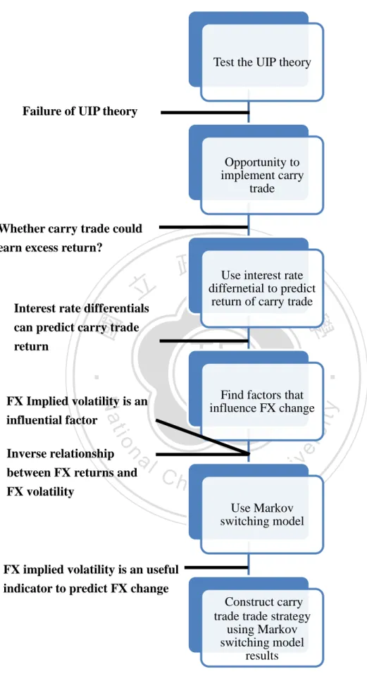
(11) Test the UIP theory. Failure of UIP theory. Opportunity to implement carry trade Whether carry trade could earn excess return?. 立. 治interest rate 政 Use 大 differnetial to predict return of carry trade. Find factors that influence FX change. n. er. io. al. Inverse relationship between FX returns and FX volatility. sit. Nat. FX Implied volatility is an influential factor. y. ‧. ‧ 國. 學. Interest rate differentials can predict carry trade return. Ch. engchi. i Un. v. Use Markov switching model. FX implied volatility is an useful indicator to predict FX change Construct carry trade trade strategy using Markov switching model results Figure 1 Framework of this paper. 11.

(12) 2. Literature Reviews 2.1 Uncovered interest rate parity (UIP). In the areas of international finance, there are three important international equations. That is, uncovered interest rate parity (UIP), purchasing power parity (PPP) and real interest rate parity. UIP theory is continuous debated in many literatures. The UIP theory explains the relationship between change in the spot exchange rate and the interest rate differentials. State differently, if UIP holds, high-interest-rate currencies tend to depreciate in the long run due to international capital movement.. 政治大. A similar concept related to UIP is covered interest rate parity (CIP). CIP holds. 立. due to the arbitrage. That is, an investment in foreign money market investment. ‧ 國. 學. instrument which is completely hedged against adverse movement of exchange rate should offer the same return as domestic money market investment instrument. If the. ‧. CIP equation doesn’t hold (assume under forward discount), arbitrage opportunity. y. Nat. sit. appears. Speculators will borrow foreign currency and convert the proceeds into home. n. al. er. io. country’s currency. They can earn a risk-free return if they deposit the proceeds into. Ch. money market instruments in home country.. engchi. i Un. v. Based on the theory, CIP always holds due of arbitrage. However, UIP doesn’t. If both UIP and CIP hold, this paper can state the uncovered interest rate parity as the relation between the change in foreign exchange spot rate and the forward rate discount (premium). Due to this relationship, previous literatures use two methods to test the UIP theory. Previous literatures have tested these two methods and find that UIP equation cannot hold over different investment period with different data frequencies. In most of the case, the slope coefficient of interest rate differential isn’t centered on one and usually shows negative sign. In this section, this paper provides the literatures both for 12.

(13) and against the UIP theory. The first part provides the journals that argue that UIP theory doesn’t hold. The second part provides the journals that propose UIP theory hold in practice.. 2.1.1 Literatures against UIP theory. Ichiue and Koyama (2011) use the Fama regression to test whether UIP equation holds in the major developed countries, include JPY, GBP, CHF and DEM. The empirical results suggest that the UIP theory fails in practice and the coefficient of the. 政治大 low-interest-rate currencies tend to depreciate and high-interest-rate currencies tend to 立. interest rate differentials in Fama regressions among all countries are negative. That is,. ‧ 國. 學. appreciate.. Lee (2013) uses the monthly currency data of both developed and developing. ‧. countries to test the UIP theory. Empirical results suggest that almost all the UIP slope. Nat. sit. y. coefficients are negative. The slope coefficients of developed countries are much. n. al. er. io. more negative than those of developing countries. The author also finds that the. i Un. v. rejection rates of UIP equation increase as the investment horizon increases.. Ch. engchi. Froot (1990) has summarized 75 journals related to UIP test. He concludes that the average slope coefficient of interest rate difference is -0.88. In theory, if UIP holds, average slope coefficient of interest rate difference equal to 1. Previous papers have different explanations of the negative beat coefficient. Some literatures comment that the negative beta coefficient may due to time-varying risk premium. Some explain this anomaly is due to expectational errors. Bansal and Dahlquist (2000) use 28 countries, with 16 developed and 14 developing countries, to test the forward premium puzzle (test of UIP). They find that forward premium puzzle tend to occur in developed countries. However, forward 13.

(14) premium puzzle isn’t significant in developing countries. They also find a state-dependence relationship between U.S interest rate and the interest rate of other countries. “Forward premium puzzle” is prone to occur when U.S interest rate is greater than other countries’ interest rate. Nevertheless, this state-dependence relationship isn’t obvious in developing countries.. 2.1.2 Literatures support UIP theory. Baillie and Bollerslev (2000) use the stylized UIP model which uses actual data. 政治大 data in this model to test UIP equation and finds that the slope coefficient of interest 立. to calibrate the model to obtain related parameter values. The author plugs in monthly. ‧ 國. 學. rate differential approximately equal to one. However, the slope coefficient is relative dispersed. So the author argues that the forward premium anomalies may due to. ‧. statistical artifact.. sit. y. Nat. Chaboud and Wright (2002) use high frequency 5 minute foreign exchange data. n. al. er. io. to test the UIP theory and find that the slope coefficient of UIP equation. i Un. v. approximately equal to one. The authors argue that the failure of UIP theory may be. Ch. engchi. due to the risk premium. When time period reduces, the risk premium also diminishes. So, high-interest rate currencies tend to appreciate and low-interest-rate currencies tend to depreciate. Lothian and Wu (2002) use two currency pairs, French franc against British pound and US dollar against sterling, for 200 years to test the UIP theory. The authors use ultra-long time period in order to prevent the results of forward-premium regressions distorting by particular sample period. The empirical results suggest that UIP holds well over long-time period. The regressions intercept of the two currency pairs is greater than zero and the slope coefficient of franc against sterling isn’t 14.

(15) significantly different from one. They conclude that UIP tends to hold in the long-run but is prone to fail in the short-run. They also find that the larger the interest rate differential between currencies pairs the greater the predictive ability for currency movement in the future. Baccetta and Wincoop (2009) make the assumptions that portfolio won’t continuously active manage their portfolio which is different from the previous literatures that they assume portfolio managers consider all relevant information immediately. Based on the “infrequent portfolio decisions” assumption, the authors propose some explanations why forward premium puzzle exists. First, as a result of. 治政 infrequent portfolio decisions, portfolio managers tend大 to follow momentum strategy 立 by buying currencies which are prone to appreciate. The authors call this phenomenon ‧ 國. 學. as “delayed overshooting”. Moreover, this “delayed overshooting” has some. ‧. predictive ability in the direction of exchange rate. Second, due to high transaction. sit. y. Nat. costs, it’s not benefit to exploit the forward premium puzzle. Furthermore, high risk. io. al. n. take risk.. er. accompanies by implementing carry trade strategy also limits investor’s willingness to. Burnside, Eichenbaum. iv n C and Rebelo use a microstructure h e n g(2007) chi U. approach to. explain the “forward premium puzzle”. They assume foreign currency market have two kinds of trader-informed trader and uninformed trader. Due to the fact that foreign exchange transaction usually takes place in OTC market, so those traders transact with market maker. Assuming that US dollar expects to appreciate against sterling, uninformed traders tend to follow the momentum trading rule and buy the US dollar forward. Informed traders possess some private information and sell the US dollar forward. Because market maker cannot distinguish between informed and uninformed traders, so he tend to charge different price for buy order and sell order based on his view on the foreign exchange. If the market maker expects the US dollar appreciate 15.

(16) against pound and receives buy order, he will charge higher quote price for the buy order. So the forward premium is high when the US dollar appreciates. This phenomenon also calls averse-selection. Averse-selection can give one explanation of the existence of forward premium puzzle. Clarida, Davis and Pedersen (2009) propose that the well-known results of negative slope coefficient in Fama regression may not hold under different volatility regime. The authors divide the sample periods into two volatility regime. One is high-volatility regime and the other is low-volatility regime. They use 9 currencies to test whether the slope coefficient of Fama regression is positive or negative. The. 治政 results show that the slope coefficient is negative in low-volatility regime. However, 大立 the slope coefficient is positive in high-volatility regime although the slope coefficient ‧ 國. 學. is negative for the entire sample period. Furthermore, the slope coefficient under. ‧. high-volatility regime is larger than 1. That is, the low-interest-rate currency is prone. sit. y. Nat. to appreciate more than implied by interest rate difference. So, the authors conclude. io. n. al. er. that the volatility-regime may give one explanation of the forward premium puzzle.. 2.2 Carry trade. Ch. engchi. i Un. v. Darrvas (2009) proposes that previous papers confirm that leverage will increase the exchange rate risk which is the major reason to drag down the return of carry trade. The author considers the leverage effect in the carry trade positions which is different from previous literatures that assume non-leverage carry trade positions. The author use not only common base currency such as us dollar and British pound and also another 9 major currencies to act as base currency. The empirical results suggest that the leverage negatively affects skewness and exhibits U-shaped relationship with the return. That is, when leverage increases to certain level, return continues to fall. The 16.

(17) major conclusion of this paper is that when carry trade position doesn’t consider leverage, excess returns tend to present. However, when positions consider leverage, the excess returns vanish. So the author argues that leverage may act as one explanation that UIP theory fails. Dunis and Miao (2007) compare three trading strategies (Benchmark MACD model, Carry model and Combined & MACD model) by using annual return, information ratio and maximum drawdown to determine which model performs best in both in-sample period and out-of-sample period. The empirical results show that carry model has the highest annual return and Sharpe ratio among three models. Then,. 治政 the authors add the volatility filters (“no trade” filter 大and reverse filter) to three 立 models. The results suggest that the combined carry/ MACD model has the lowest ‧ 國. 學. maximum drawdown among three models. They also find that strategy equipped with. ‧. volatility filter has lower maximum drawdown than strategy without volatility filter.. io. er. volatility of carry trade’s return significantly.. sit. y. Nat. So they conclude that adding volatility filter to carry trade strategy can reduce. al. Becker and Clifton (2007) extend previous literatures to find the relationship. n. iv n C between hedge fund activities and h carry trade strategy. e n g c h i U However, due to limited data of hedge fund returns and related activities, former papers usually use indirect data to draw statistical inference. The authors use the banking data from BIS to proxy for hedge fund data. They use Japanese yen and Swiss Franc to act as funding currency and use the 10-year government bond yields of Australia and New Zealand to calculate the profits hedge fund may earn. Due to large amounts of money to implement carry trade, capitals of hedge fund flow into high-yield currencies usually cause exchange rate to appreciate. However, when the exchange rate volatility increases, hedge funds tend to unwind their positions which may cause turmoil in foreign exchange markets. 17.

(18) Clarida, Davis and Pedersen (2009) use the G10 currencies to examine the relationship between return and risk of the carry trade positions. They calculate the realized volatility by using exponentially weighted moving averages (EWMA). They define the low-volatility regime if the realized volatility is less than 25th percentile for the entire sample period and the high-volatility regime if the realized volatility exceeds 75th percentile for the entire sample period. The results show that returns are higher under low-volatility regime than those under high-volatility regime. The authors also use the Kernel regressions, a non-parametric method, to do the robustness check. The findings are consistent.. 治政 Brunnermeier, Nagel and Pedersen (2009) argue that 大 high-interest rate currencies 立 are subject to currency crash. That is, high-interest rate currencies tend to appreciate ‧ 國. 學. in short notice. Although failure of uncovered interest rate parity let carry trade. ‧. strategy earn excess return on average, high-interest rate currencies depreciate. sit. y. Nat. abruptly could have negative impact on carry trade positions. The authors propose. io. er. that high-interest rate currencies such as AUD and NZD tend to have conditional. al. negative skewness. This paper knows that under the statistical properties, asset returns. n. iv n C with negative skewness are prone to negative returns. So high-interest hhave e nextremely gchi U tare currencies with negative skewness are consistent with our observation in FX. market. Then, the authors use the simple regressions to examine the relationship between quarterly carry trade return, interest rate difference mince change in log return on FX, and the interest rate differential. They find that the slope coefficient of regressions is positive. This implies that positive returns could be predicted by high interest rate differences. The authors also run the OLS regressions to test the relationship between futures positions held by speculators and interest rate differential. The result shows that speculators such as hedge funds tend to hold large long 18.

(19) positions in high-interest rate currencies. This observation also could act as another explanation that UIP theory doesn’t hold. Fong (2013) uses the data from Commodity Futures Trading Commissions (CFTC) to examine whether hedge funds have significant impact on FX markets or not. The preliminary analysis of this paper suggests that hedge funds have net positive positions in high-interest-rate currencies such as AUD and NZD and have net negative positions in low-interest-rate currencies such as EUR and USD. This observation is consistent with what this paper observed in the FX market. That is, the hedge funds usually try to exploit UIP failure to make profits. Then, the author use both OLS regression and structural VAR. 立. 治政 model to examine 大 whether. hedge funds follow. momentum strategy. To state differently, this paper wants to examine whether hedge. ‧ 國. 學. funds exhibit trend chasing behavior or not. The empirical results are consistent with. ‧. previous papers that hedge funds indeed follow momentum strategy. Finally, the main. sit. y. Nat. contribution of this paper is to examine whether hedge funds activities will impact FX. io. er. market or not. The author uses Quantile regression to divide the data into low. al. quantiles (represent normal market) and high quantiles (represent turbulent market). n. iv n C and test the relationship between h future FX returnsUand hedge fund net positions. engchi Under turbulent market, the coefficients of the hedge funds net positions are negative among all six currencies. In particular, the coefficients of AUD and NZD in terms of absolute value are greater than those of other currencies. Under normal market, the coefficients of the hedge funds net positions are positive and mostly insignificant among all six currencies. These two results imply that hedge fund activities have a reversal effect on FX market under turbulent market and virtually no impact under normal market.. 19.

(20) 2.3 Markov Switching model Ichiue and Koyama (2011) use the four-regime model to examine the relationship between interest rate and foreign exchange. They use the slope regime and volatility regime to categorize four-regime. In other words, they divide slope regime into high-slope state and low-slope state and divide volatility regime into high-volatility state and low-volatility state. For example, regime 1 is defined as low-slope state and low-volatility regime. Regime 2 is defined as low-slope state and high-volatility regime. The empirical results have the following implications. First, slope coefficients of the interest rate differential are negative under low-volatility state. 治政 and positive under high-volatility state. This implies 大 that the magnitude of 立 appreciation of the low-interest-rate currency is larger than that of depreciation. The ‧ 國. 學. authors also find that the unconditional probability of the negative and low regime is. ‧. larger than 0.58 in eight cases. These two empirical findings are consistent with what. sit. y. Nat. this paper observes in FX market. That is, low-rate currencies tend to depreciate over. io. al. er. time. However, low-rate currencies appreciate less frequently but with significant. n. magnitudes, which is also one important reason why carry trade strategy is so prevalent.. Ch. engchi. i Un. v. 3. Methodology 3.1 The forward premium anomalies Assuming that uncovered interest rate parity (UIP) holds and investors are risk neutral, changes in FX spot rate over the investment period should equal to the interest rate differential between two countries. This paper expresses UIP as followed: (1 + 𝑖𝑓 ) ∗ (1 − ∆𝑆𝑓/𝑑 ) − 1 ≒ 𝑖𝑓 − ∆𝑆𝑓/𝑑 = 𝑖𝑑. 20.

(21) 𝑖𝑓 and 𝑖𝑑 stand for interest rate for foreign country and domestic country, respectively. ∆𝑆𝑓/𝑑 stands for changes in FX spot rate. If investors form a portfolio by holding foreign money market assets and fully hedging the FX risk, then the return of this portfolio should equal to the return offered by domestic money market instruments. In equilibrium, CIP holds due to arbitrage. This paper expresses CIP as followed: 𝑆𝑓/𝑑 * (1 + 𝑖𝑓 ) * (𝐹𝑓/𝑑 −𝑆𝑓/𝑑 ) 𝑆𝑓/𝑑. 𝑆𝑓/𝑑. 1 𝐹𝑓/𝑑. = (1 + 𝑖𝑑 ). is forward premiums/ discounts ≒ (𝑖𝑓 − 𝑖𝑑 ). 政治大. and 𝐹𝑓/𝑑 stand for spot FX rate and forward rate, respectively.. 立. 學. ‧ 國. This paper knows that CIP always holds due to arbitrage. However, UIP may not hold all the time because investors may not exhibit risk-neutral preference. If this paper assumes that UIP holds, then the following equation holds:. sit. y. ‧. Nat. (𝐹𝑓/𝑑 − 𝑆𝑓/𝑑 ) = (𝑖𝑓 − 𝑖𝑑 ) = ∆𝑆𝑓/𝑑 𝑆𝑓/𝑑. io. er. In order to test whether UIP holds or not, this paper examines the relationship. al. between the first and third terms or the second and third terms in the above equation.. n. iv n C This paper chooses to examine UIPhtheory by using U e n g c h i the second and third terms. That is, the relationship between interest rate differential and change in FX spot rate.. Previous literatures test UIP theory using different time periods and currencies. Many literatures find evidence against UIP theory. In this section, this paper updates new time periods and uses both the currencies of developed and developing countries to examine whether UIP theory holds or not. Many literatures use the regression model proposed by Fama (1984) to test the so-called “forward discount anomalies”. That is, UIP theory fails in practice. This model is also called Fama regression. This paper defines Fama regression as follows: 21.

(22) 𝑦𝑡+𝑖 − 𝑦𝑡 = α0 + β1 (𝑟𝑡,𝑑 − 𝑟𝑡,𝑓 ) + 𝜀𝑡+𝑖 Where 𝑦𝑡+𝑖 stands for log nominal exchange rate of domestic currency relative to foreign currency at time t+i, and 𝑟𝑡,𝑑 and 𝑟𝑡,𝑓 stand for domestic and foreign interest rate, respectively. 𝜀𝑡+𝑖 is white noise and follows normal distribution. If UIP holds, α0 and β1 should equal to 0 and 1, respectively. This paper uses Wald test to examine whether the null hypothesis that α0 = 0 and β1 = 1 can be rejected. 3.2 Interest rate differential predicts returns of carry trade. 治政 Brunnermeier, Nagel and Pedersen (2009) use the 大carry interest to predict the 立 future performance of carry trade strategy for the next two and a half years. This ‧ 國. 學. paper uses the same methods as in Brunnermeier, Nagel and Pedersen (2009) but. ‧. different currency pairs and time periods to examine whether high interest rate. sit. y. Nat. differential could predict future returns of carry trade during the next few quarters. This paper defines the logarithm of the FX rate (indirect quotation) as followed:. er. io. rt =a log (𝑓𝑜𝑟𝑒𝑖𝑔𝑛 𝑒𝑥𝑐ℎ𝑎𝑛𝑔𝑒 𝑟𝑎𝑡𝑒). n. iv l C n Then, this paper defines the carry return and denotes Rt+1 as the interest rate h etrade ngchi U differential between high- and low-interest rate currency adjusted for averse FX movement. This paper defines the equation as follows:. Rt+1 ≣ (𝑖1𝑓 − 𝑖1𝑑 ) − ∆ 𝑟𝑡+1 This paper wants to know whether interest rate differnetial could predict carry trade return for the next few quarters, this paper runs the following regressions:. Rt+i = α0 + β1 (𝑖𝑡𝑓 − 𝑖𝑡𝑑 ) + 𝜀𝑡 Brunnermeier, Nagel and Pedersen (2009) use the interest rate differential to predict the carry trade returns over next two and a half years. That is, using interest rate differential to predict next 10 quarters. However, this paper only predicts the 22.

(23) carry trade returns over next one year. As this paper will mention in the section “Interview with trader in domestic bank FX trading desk”, the investment periods are at most one year. So, this paper uses carry interest to predict the returns for the next year (next four quarters). 3.3 Using OLS to find influential factors Previous literatures show that although carry trade may earn excess return on average, it also accompanies with significant downside risk. That is, the appreciation of low-interest-rate currency. According to carry trade structure, investors borrow. 治政 low-interest-rate currency to fund high-interest-rate 大 investment. In essence, carry 立 trade is a leverage position. When low-rate currency appreciates sharply, investors ‧ 國. 學. need to pay more money to offset their short position. Furthermore, the leverage effect. ‧. magnifies the negative effect on return of carry trade.. sit. y. Nat. In order to control FX adverse movements, this paper uses the multiple. io. er. regressions to find variables that could explain the FX adverse change. Observing the. al. FX market, many FX participants monitor the FX market by gauging FX implied. n. iv n C volatility. Based on this observation theory, this paper chooses interest rate h eandnUIP gchi U differential and FX at-the-money implied volatility to act as independent variables. This paper specifies the multiple regressions as followed: (𝑌𝑡+𝑛 − 𝑌𝑡 ) = α0 + β1 (𝑟𝑓,𝑡,𝑛 − 𝑟𝑑,𝑡,𝑛 ) + β2 (𝐹𝑋σ𝑡 ) + є𝑡+𝑛 𝑌𝑡 : log of FX spot rate 𝑟𝑓,𝑡,𝑛 − 𝑟𝑑,𝑡,𝑛 : interest rate differential 𝐹𝑋σ𝑡 : FX at-the-money implied volatility є𝑡+𝑛 ~ N (0,σ2 ). 23.

(24) 3.4 Two-stage Markov switching model Bekaert and Hodrick (1990) use a two-regime model and choose interest rate differential as an independent variable. Ichiue and Kentaro (2011) employ a four-regime model and also select interest rate differential as an independent variable. This paper augments the two-regime model by adding FX implied volatility as an additional independent variable. This paper expresses two-stage regime-switching model and defines the related variables as followed: (𝑌𝑡+𝑛 − 𝑌𝑡 ) = α𝑖 + β𝑖 (𝑟𝑓,𝑡,𝑛 − 𝑟𝑑,𝑡,𝑛 ) + β𝑗 (𝐹𝑋σ𝑡 ) + σ𝑖 є𝑡+𝑛 , i =1, 2. 政治大 : interest rate differential 立. 𝑌𝑡 : log of FX spot rate 𝑟𝑓,𝑡,𝑛 − 𝑟𝑑,𝑡,𝑛. ‧ 國. 學. 𝐹𝑋σ𝑡 : FX at-the-money implied volatility σ𝑖 : Realized FX volatility. ‧. є𝑡+𝑛 ~ N (0, 1). Nat. sit. y. This paper provides some reasons why including FX implied volatility in the. n. al. er. io. regime-switching model. First, FX implied volatility has forward-looking feature.. i Un. v. That is, FX implied volatility not only includes recent information in FX market, it. Ch. engchi. also reflects the market expectation in the future. For example, 6-month FX implied volatility includes the expectation held by most of the FX market participants. Second, in the preliminary analysis in OLS regressions, FX implied volatility is statistically significant variable in all eight currencies in different investment period. So this paper believes that FX implied volatility could explain the change in FX spot rate. In the Markov-switching model, this paper uses at-the-money (ATM) FX implied volatility. Some may argue that why this paper uses ATM FX implied volatility rather than out-of-the-money (OTM) implied volatility? This paper proposes some reasons. First, the objective in this paper is to find some indicators to control the risk of carry 24.

(25) trade and enhances its return. This paper wants to find some variables that could reflect current or future market circumstances. However, OTM FX implied volatility reflects not only future outlook related to FX market but also includes hedging effect. For example, some institutions may want to hedge their FX exposures using OTM options. Some carry trade traders may only want to earn interest rate differentials and hedge their FX positions using OTM options. Due to the reasons mentioned above, this paper chooses ATM FX implied volatility to be an independent variable. 3.5 Constructing carry trade strategy 3.5.1.1 Interview with FX trader in domestic bank. 立. 政治大. In order to construct the carry trade strategy that is closely aligned with what FX. ‧ 國. 學. trader actually do in practice, this paper interviews with one of my seniors in Department of International Business, National Chengchi University (NCCU). This. ‧. paper summarizes the 30 minutes interview in the following six questions.. y. Nat. n. al. er. io. strategy?. sit. Question 1: What are the average investment periods of the carry trade. Ch. i Un. v. Carry trade strategies can be categorized into two forms:. engchi. 1. The first type of strategy focuses on FX forecasting and FX volatility. That is, the major return contributions come from favorable FX change. Due to the fact that FX market tends to be volatile, so this kind of strategy has relative short investment period. 2.. The second type of strategy focuses on earning long-term interest rate differential. In order to increase the interest income revenues, the investment period of this kind of strategy is longer than the first type of strategy. The traders usually hold the positions for 6 to 12 months. The reason is that the longer the holding period, the higher the interest income earned. For example, if a trader 25.

(26) have 100 million USD dollar on hand, and invest in LIBOR for one year. If interest rate is one percent, trader can earn only 1 million interests per year. Furthermore, due to the economic recession during the past few years, many governments implement aggressively monetary policy such as quantitative easing to reduce the interest rate. Those monetary policies also reduce the interest rate differential of carry trade strategy. In practice, the common holding period of carry trade position is at least 6 months but no longer than 12 months. Question 2: Generally, what is the regular one-time trading amount that a FX trader implements carry trade strategy?. 治政 In practice, international institutional investors 大 usually implement carry trade 立 strategy with trading volume at least USD 50 million to USD 100 million at one time. ‧ 國. 學. For small institutional investors, the trading volume is at least USD 1 million. The. ‧. reason of large trading volume is the same as Question 1. Furthermore, this one-time. sit. y. Nat. large trading volume could have a significant impact on FX markets. The magnitude. io. al. er. of market impact is a function of market depth. The market depth can be measured by. n. daily trading volume of FX market.. Ch. i Un. v. Table 1 Daily trading volume of spot rate of major currencies in FX market. engchi. Currency pair (against USD). Daily trading volume of spot rate (millions). Euro. 105,227. Japanese yen. 66,892. Australia dollar. 25,500. Swiss franc. 14,488. Mexican peso. 13,955. Brazil real. 3,744. All other currencies. 35,414 26.

(27) Source: foreign exchange committee semi-annual foreign exchange volume survey Oct 2013 Table 1 is the daily trading volume of the major currencies in FX market. The amounts are averaged over twenty three trading days in October 2013. Observing from Table 1, the major currencies have high trading volume. This also implies low liquidity risk and low market impact. However, the common target currencies such as NZD and emerging market currencies have relatively low daily trading volume. So, when traders select NZD and emerging market currencies as investment targets, transaction costs due to market impact will be huge.. 政治大 when implementing carry立 trade strategy?. Question 3: What other types of transaction costs incur besides bid-ask spread. ‧ 國. 學. Besides bid-ask spread, other transaction costs include broker commission fees and transaction costs due to market impact. The average transaction costs account for. ‧. 1 to 2 basis points of total trading volume if trader buys USD 100 million foreign. Nat. sit. n. al. er. io. trading amount.. y. currencies at one time. Therefore, commission fees are relatively small due to large. i Un. v. So, this paper concludes that the major transaction costs include both bid-ask. Ch. engchi. spread in normal market and in distressed market.. Question 4: What kinds of interest rate do large international institutional investors borrow and invest to implement carry trade in practice? International institutional investors usually borrow low-interest-rate currency through LIBOR and invest in different interest rate in different countries. So, the borrowing rate is different from the investment rate. However, most data related to borrowing rates are unavailable, so in our paper, this paper assumes borrowing rate is equal to investment rate which can be represented by LIBOR. Question 5: What is the best timing to implement carry trade strategy? 27.

(28) Different traders use various indicators or tools to determine when to implement carry trade. The following signals are frequently used by traders in practice. 1. When low-rate currency depreciates against high-rate currency, this may be an opportunity to implement carry trade. For example, U.S. dollar depreciates against Australia dollar, then the trader can borrow cheap U.S. dollar and invests in Australia dollar which has potential to appreciate in the future. 2. If central bank of high-rate country raises interest rate, this government action implies not only the increase in interest rate differential but also potential appreciation of the FX of high-rate country due to large capital inflow.. 治政 The two signals mentioned above also mean that the大 major return contributions of 立 carry trade come from interest rate differential and FX favorable change. ‧ 國. 學. Question 6: How do traders hedge the FX risk that investment currency. ‧. depreciates abruptly?. sit. y. Nat. Different institutional investors gauge different indicators to monitor FX. io. er. positions and manage FX risk. FX traders pay closely attention on the announcement. al. of central bank monetary policy and some macroeconomic factors such as nonfarm. n. iv n C employment, unemployment rate, PMI consumer confidence index, and so on. h eindex, ngchi U 3.5.1.2. Short conclusion of the interview. 1. Investment period is at least 6 months but no more than 12 months. 2. One-time trading amount equals to USD 50-100 million. 3. Investment currencies include AUD, NZD, MXN, REAL. 4. Both borrowing and investing rate are LIBOR. 5. The timing to implement carry trade includes: (1) low-rate currency depreciates against high-rate currency 28.

(29) (2) Interest rate differential between two countries increases 6. Different institutions gauge different indicators to monitor FX risk. 3.5.2 Determine the timing to implement and close out carry trade positions. This paper chooses two developed market currencies (AUD and NZD) and two developing market currencies (MXN and REAL) to act as investment currencies due to their high daily trading volume. So this paper uses these four currencies to examine the performance of carry trade strategies this paper constructs.. 政治大 The first part is the best timing to implement carry trade strategy. The second part is 立 This paper divides the process of carry trade strategy construction into two parts.. ‧ 國. 學. the timing to close out carry trade positions. Investors realize profit or stop losses when receiving trading signals.. ‧. The best timing to implement carry trade strategy. io. sit. y. Nat. 3.5.2.1. n. al. er. According to the practice of FX traders gained through an interview, this paper. Ch. i Un. v. assumes the firms that implement carry trade strategy are large foreign financial. engchi. institutional investors. We know that the LIBOR is the interest rate borrowed and lent in the London interbank. Only large financial institutions with great creditability can borrow funds at LIBOR rate. This paper further assumes that the firms that implement carry trade focus on interest rate differential. Therefore, the investment period is at least 6 months. This paper also assumes the one-time trading volume is 100 million, so this paper takes the transaction costs under normal and distressed conditions in to consideration. This paper constructs the carry trade strategy as followed: If the following two conditions are met simultaneously, this paper implements the carry trade strategy. 29.

(30) 1. The Interest rate differential between two countries increases due to increase in the interest rate of investment currency For example, if the interest rate differential between Australia and America increases and interest rate of Australia increases, this paper implements carry trade strategy.. 2. Low-rate currency depreciates against high- rate currency For example, if US dollar depreciates against Australia dollar, then it’s profitable to borrow cheap U.S dollar and invest in Australia dollar. This concept may seem. 政治大. simple and intuition. However, by what magnitude low-rate currency depreciates. 立. against high- rate currency could investors confirm that low-rate currency is in. ‧ 國. 學. depreciating trend? This paper defines a threshold to verify that low-rate currency is in the trend of depreciation. In practice, FX traders usually use moving average to. ‧. predict the trend of foreign exchange. So the decision rule is as follows:. y. Nat. io. sit. Decision rule: if current spot FX rate is less than 20-day moving average FX rate,. n. al. er. this situation satisfies condition 2.. 3.5.2.2. Ch. engchi. i Un. v. The best timing to close out carry trade strategy. This paper constructs the following three strategies and compares their performance according to Sharpe ratio with the performance benchmark to determine which strategy performs best in different sample periods. This paper divides the sample period into in-sample period and out-of-sample period to confirm the robustness of the strategies. Strategy 1―Buy-and-hold to maturity 1. The traders hold the carry trade positions for at least specific months and then close out the positions. Strategy 1 is passive strategy because traders don’t need to 30.

(31) make any tactical adjustment to reflect short-term changes in FX market. As this paper has mentioned in the section of interview with FX traders, the investment period of carry trade can be short-term (focus on short-term FX volatility) and long-term (focus on interest differential). Our major focus here is interest rate differential, so this paper requires the investment period of carry trade should at least 6 months but no longer than 1 year. 2. Buy-and-hold strategy usually acts as performance benchmark. As this paper will mention later, Strategy 2 and Strategy 3 hold the positions at least 6 months but no longer than 12 months. So, the investment periods of these two strategies are. 治政 within 6 to 12 months. So, this paper chooses Buy-and-hold 大 strategy for 6 months 立 and 12 months to act as performance benchmarks. ‧ 國. 學. Decision rules: Buy and hold the carry trade positions for 6 and 12 months .Then. ‧. until maturity, this paper closes out carry trade positions.. y. Nat. io. sit. Strategy 2―Using FX implied volatility. n. al. er. This paper has examined in the previous OLS regressions that FX implied. Ch. i Un. v. volatility can explain the future change in FX rate. Furthermore, FX implied volatility. engchi. is a forward-looking measure that reflects both the market consensus of participants, including informed traders, and contains all relevant information. This paper uses at-the-money (ATM) FX implied volatility to gauge the current FX market volatility. Some people may argue that why you choose ATM implied volatility rather than out-of-the-money (OTM) implied volatility. If short-term FX implied volatility breaches long-term FX implied volatility, this may provide a signal that FX market shifts from low-volatility state to high-volatility state. This paper chooses 20-trading-day FX implied volatility to stand for short-term. 31.

(32) FX implied volatility and selects 240-trading-day FX implied volatility to act as long-term FX implied volatility. Decision rule: if short-term implied volatility (20-day) breaches longer-term implied volatility (240-day), this paper closes out the carry trade positions.. Strategy 3―Using FX implied volatility and the results of Markov switching model (Combination strategy) Strategy 3 includes not only the decision rule in Strategy 2 but also the empirical results this paper gained in Markov-switching model.. 治政 The two-stage Markov-switching model divides 大 the whole sample into 立 low-volatility state (state 1) and high-volatility state (state 2). The results of ‧ 國. 學. Markov-switching model show that the coefficients of implied volatility in AUD/USD,. ‧. NZD/USD and USD/MXN under state 2 are higher than that under state 1.. sit. y. Nat. The coefficient of FX implied volatility in USD/REAL under state 1 is higher. io. er. than under state 2. This means that when the FX implied volatility under state 2 (or state 1) is high, the high-interest-rate currency tends to depreciate against. al. n. iv n C low-interest-rate currency. If FX h traders observe this e n g c h i U situation, they could quickly close out the carry trade positions to hedge the FX risk. Decision rules: (1) Based on the results showed in Markov-switching model, FX implied volatility of AUD, NZD and MXN is higher in State 2 than in State 1 and FX implied volatility of REAL is higher is State 1 than in State 2. (2) When current market is in State 1 (for AUD, NZD and MXN) or State 2 (REAL) and 20-day implied volatility breaches 240-day implied volatility, this paper closes out the carry trade positions. 32.

(33) 3.5.2.3. Determine the future state of Markov-switching model. The following methods refer to Young (2013). In order to determine whether the three carry trade strategies are valid, this paper uses in-sample and out-of-sample periods to test their performances. This paper defines the period between Jan 2000 to Dec 2012 as the in-sample period and the period between Jan 2013 to Dec 2013 as the out-of-sample period for eight currencies except NZD and AUD. Due to data unavailability, this paper defines the period between Jan 2000 and June 2012 as the in-sample period and set the period between Jul 2012 and June 2013. 政治大. as the out-of-sample period for AUD. this paper defines the period between Jul 2003. 立. and Feb 2012 as the in-sample period and set the period between Mar 2012 and Feb. ‧ 國. 學. 2013 to be out-of-sample period for NZD.. This paper provides the in-sample-period and out-of-sample period among eight. Nat. In-sample period. al. Out-of-sample period. er. io. i v 2012 – Jul n U. Jun 2013. Mar 2012 –. Feb 2013. Jan 2000 – Dec 2012. Jan 2013 –. Dec 2013. Jan 2000 – Dec 2012. Jan 2013 –. Dec 2013. n. Currency. sit. Table 2 In-sample-period and out-of-sample period for four currencies. y. ‧. currencies in Table 2.. AUD. Jan 2000 – Jun 2012. NZD. Jul 2003 – Feb 2012. MXN REAL. Ch. engchi. This paper uses the expected probability to determine which state is more likely in the future. The equation for expected probability is as followed: 2. Expected probability = Prob(𝑠𝑡+1 = 𝑦|𝐼𝑡 , 𝜃) = ∑ Prob(𝑠𝑡 = 𝑥|𝐼𝑡 , 𝜃) ∙ 𝑝𝑖𝑗 𝑥=1. 𝐹𝑖𝑙𝑡𝑒𝑟 𝑝𝑟𝑜𝑏𝑎𝑏𝑖𝑙𝑖𝑡𝑦 = Prob(𝑠𝑡 = 𝑥|𝐼𝑡 , 𝜃) 𝑝11 𝑇𝑟𝑎𝑛𝑠𝑖𝑡𝑖𝑜𝑛 𝑝𝑟𝑜𝑏𝑎𝑏𝑖𝑙𝑖𝑖𝑡𝑦 = 𝒑𝑖𝑗 = [𝑝 21 33. 𝑝12 𝑝22 ].

(34) For example, filter probability of time t under State 1 and State 2 are (0.985, 0.015). Transition probability is [. 0.996 0.004. 0 ]. 1. Multiplying filter probability by transition probability obtains expected probability which equals (0.98525 0.01475). Based on expected probability, this paper expects that State 1 is more likely to occur in time t+1 due to high expected probability. Due to the computational complexity and some technical problems, this paper smooth the variables required to calculate filter probability and transition probability. 政治大 change in log of foreign exchange rate, interest rate differential, and FX implied 立 using 5-day the moving average of the preceding 5 days of related variables, include. ‧ 國. Transaction costs. ‧. 3.5.2.4. 學. volatility.. y. Nat. io. sit. Due to imperfect market, this paper takes transaction costs into account as. n. al. er. implementing carry trade. This paper divides transaction costs into three parts. 1. Brokerage commissions. 2. Bid-ask spread.. Ch. engchi. i Un. v. 3. Market impact due to one-time large trading volumes. According to previous literatures, almost all papers assume perfect market. That is, they assume there are no taxes, transaction costs and related constraints. However, in practice, transaction costs could significantly affect carry trade returns. In our paper, this paper assumes imperfect market and takes transaction costs into account. According to interview with FX trader, this paper assumes the one-time trading amount is 100 million. This paper ignores the brokerage commissions (only account for 1 to 2 basis points). This paper uses the daily FX data during period of Jan 2000 to 34.

(35) Dec 2013 to calculate average bid-ask spread ratio and provide the equation as follows: Bid-ask spread ratio = ( Mid-price = (. 𝒂𝒔𝒌 𝒑𝒓𝒊𝒄𝒆−𝒃𝒊𝒅 𝒑𝒓𝒊𝒄𝒆 𝒎𝒊𝒅 𝒑𝒓𝒊𝒄𝒆. ). 𝒂𝒔𝒌 𝒑𝒓𝒊𝒄𝒆+𝒃𝒊𝒅 𝒑𝒓𝒊𝒄𝒆. ). 𝟐. Table 3 Transaction cost - bid-ask spread ratio (bps) Currency. JPYUSD. CHFUSD. USDNZD. USDAUD. Bid-ask spread ratio. 4.77. 4.88. 10.28. 6.71. Currency. MXNUSD. REALUSD. ZARUSD. INDUSD. Bid-ask spread ratio. 21.67. 98.77. 42.90. 49.69. 政spread治 Table 3 calculates the bid-ask ratio for大 eight currencies. This paper 立 observes that the bid-ask spread ratios of developing markets under normal condition. ‧ 國. 學. are five to ten times more than those of developed countries.. ‧. With respect to transaction costs due to one-time large trading volume, market impact needs to be taken into account. Because it’s difficult to measure transaction. y. Nat. er. io. sit. costs due to market impact precisely, this paper implements sensitivity analysis. This paper doubles and triples bid-ask spread ratio in normal condition to account for this. n. al. effect.. Ch. engchi. i Un. v. Another issue is that institutions enjoy favorable bid-ask spread ratio relative to individuals. The investors in this paper focus on institutions. 3.5.2.5. Income tax and capital gain tax. The returns of carry trade come from two parts. One comes from interest income. Another comes from capital gain due to FX change. This paper assumes that the head-quarters of institutional investors are based in America and taxed according to U.S tax rules. According to U.S tax rules, corporate tax rate is 35%. With respect to capital 35.

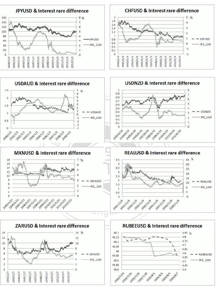
(36) gain, the tax rate depends on the holding periods. If investors close out carry trade position for one year or less, this profit is considered a short-term capital gain and is taxed at the ordinary income tax rate (35% for U.S corporates). This paper assumes that both interest incomes and capital gain income are taxed at a rate of 35%.. 4. Data description. This paper collects daily foreign exchange rate against U.S. dollar (USD) and. 政治大 volatility from Datastream during 2000 to 2013 for four developed markets and four 立 1-month, 3-month, 6-month and 12-month interbank interest rates and FX implied. ‧ 國. 學. developing markets: Japan (JPY), Switzerland (CHF), Australia (AUD), New Zealand (NZD), Mexico (MXN), Brazil (REAL), South Africa (ZAR) and India (RUBEE).. ‧. This paper presents the descriptive statistics in Table 4. Some data, emerging. sit. y. Nat. countries in particular, aren’t available for certain periods. So the observations may. n. al. er. io. not be equal among eight countries. Basically, the time periods of eight currencies. i Un. v. include major financial events such as subprime crisis, financial crisis and European. Ch. engchi. debt crisis. In Table 5, this paper provides the descriptive statistics, both expected value and standard deviation, of these three variables for eight currencies. In Figure 2, this paper provides the time series of foreign spot rate and interest rate differential for eight currencies. 36.

(37) Table 4 Mean and standard deviation of FX spot rate among eight foreign currencies, include JPY, CHF, AUD, ZND, MXN, REAL, ZAR, and RUBEE from January 3, 2000, to December 2, 2013 Currency. Mean of FX. Standard deviation of FX. 1.3481 112.6175 11.8203 2.3017 46.1883 0.6973. 0.2193 9.0416 1.1272 0.5519 3.8736 0.1243. 0.7101 7.5412. 0.0767 1.2802. JPY CHF AUD NZD MXN REAL ZAR RUBEE. 立. ‧ 國. 學. Table 5. 政治大. Mean of. Standard. y. period. interest rate. deviation. 1. 0.2189. 0.2367. sit. 0.2821 0.3577 0.4687. 0.2797 0.3035 0.3442. 1. 1.1394. 3 6 12. 0.046 0.057 0.083. 1.1209. 3.552. -0.02. 1.2434 1.3309 1.5330. 1.1534 1.1556 1.1227. 3.59 3.768 3.975. 0.003 0.043 0.239. 1. 5.2516. 0.9764. 8.213. 3.116. 3 6 12. 5.3455 5.4561 5.6839. 0.9993 0.9867 0.9717. 8.053 8.205 8.735. 3.166 3.25 3.542. Ch. engchi U. 37. er. 1.094 1.19 1.33. al. n. AUD. Min 0.0363. 3 6 12 CHF. Max 1.06. io. JPY. Measurement. Nat. Currency. ‧. Descriptive statistics of interest rate of eight foreign currencies, include JPY, CHF, AUD, ZND, MXN, REAL, ZAR, and RUBEE from January 3, 2000, to December 2, 2013 (percentage). v ni.

(38) 2.2770. 10.1. 2.6475. 3 6 12. 5.4498 5.5767 5.8342. 2.2608 2.1865 1.9916. 9.5375 9.3785 9.3425. 2.73 2.905 3.275. 1. 5.9796. 1.7907. 9.81. 3.35. 3 6 12. 6.1380 6.2779 6.4377. 1.8094 1.7805 1.7538. 10.08 10.21 10.26. 3.4 3.46 3.53. 1. 13.916. 4.897. 26.90. 5.575. 3 6 12. 13.969 14.094 14.416. 4.978 5.101 5.424. 27.77 28.69 32.56. 6.98 6.99 6.94. 1. 8.0377. 2.5040. 13.1. 4.931. 3 6 12. 8.2040 8.3640 8.6324. 2.5521 2.5145 2.4865. 13.598 13.929 14.433. 5.063 5.213 5.345. 1 3 6 12. 4.8094 6.2339. 0.5674 0.8347. io. n. al. Ch. i Un. i e n g c h 1.3863. 7.4998. ‧. Nat. RUBEE. 學. ZAR. ‧ 國. 立. 政治大. y. REAL. 5.3376. sit. MXN. 1. er. NZD. v. 5.5 7.25 9 9. 4 5 5.25 5.5. Table 6 Descriptive statistics of FX implied volatility of eight foreign currencies, include JPY, CHF, AUD, ZND, MXN, REAL, ZAR, and RUBEE from January 3, 2000, to December 2, 2013 Currency JPY. Measurement period. Mean of IV. Standard deviation. 1. 10.59. 3.02. 0.388. 0.058. 3 6 12. 10.57 10.68 10.84. 2.53 2.33 2.28. 0.26 0.1435 0.1435. 0.062 0.1435 0.1435. 38. Max. Min.

(39) 2.61. 0.2473. 0.0512. 3 6 12. 11.09 11.20 11.30. 2.38 2.17 2.10. 0.2408 0.2005 0.201. 0.055 0.0592 0.06075. 1. 14.38. 7.38. 0.66. 0.0548. 3 6 12. 14.26 14.32 14.38. 6.22 5.72 5.45. 0.54 0.45 0.41. 0.0587 0.0665 0.0694. 1. 13.47. 4.43. 0.405. 0.0845. 3 6. 13.35 13.18. 4.26 4.41. 0.3153 0.29. 0.087 0.08975. 0.27. 0.092. 0.75. 0.0465. 0.5201 0.4294 39.63. 0.0505 0.056 6.3. 立. 12. 3 6 12. 11.32 11.59 11.9558. 5.52 5.18 4.7594. 1. 16.2. 8.8. 3 6 12. 16.1 16.4 17.1. 7.3 6.7 6.1. 1. 17.78. 3 6 12 1 3 6 12. ‧ 國. 6.53. io. RUBEE. al. n. ZAR. ‧. 11.27. 學. REAL. 1. Nat. MXN. 政治大 13.78 3.20. y. NZD. 10.93. 0.6374. 0.053. 0.491 0.46 0.45. 0.0675 0.0835 0.096. 5.47. 0.7. 0.103. 17.58 17.65 17.79. 4.10 3.54 3.16. 0.47 0.42 0.35. 0.1195 0.125 0.1325. 7.60 7.54 N/A 7.50. 3.69 3.36 N/A 3.08. 0.27 0.22 N/A 0.1885. 0.01 0.01875 N/A 0.023. Ch. engchi. 39. sit. AUD. 1. er. CHF. i Un. v.

(40) 立. 政治大. ‧. ‧ 國. 學. n. er. io. sit. y. Nat. al. Ch. engchi. i Un. v. Figure 2 the time series of FX spot rate and interest rate differential (against USD). 40.

(41) 5. Empirical Results 5.1 The forward premium puzzle This paper examines the forward premium puzzle among eight currencies in different investment periods (1-month, 3-month, 6-month, and 12-month) by using Fama regressions. In Table 7, the results show that all currencies in different periods reject the null hypothesis that alpha equal to zero and beta equal to one. This paper concludes that all eight currencies reject the UIP theory during the sample periods this paper specified.. 政治大 different currencies in different investment periods are statistically significant and 立. In Table 8, this paper observes that almost all interest-rate slope coefficients of. ‧ 國. 學. their values are negative. These results are consistent with the previous literatures. That is, the average coefficients of interest rate differential are different from zero and. ‧. their values are negative. Froot (1990) summarizes the previous empirical results of. Nat. sit. y. UIP test and find that the average coefficient of interest rate differential is -0.88.. n. al. er. io. The failure of UIP theory implies that most of the time, low-interest-rate. i Un. v. currencies tend to depreciate and high-interest-rate currencies tend to appreciate. This. Ch. engchi. phenomenon results in the prevalence of carry trade. Many international institutions implement carry trade by borrowing low-rate currency and invest in high-rate currency. Could carry trade strategy make a profit on average over time? This paper will examine the return of carry trade in details in the next sections. 5.2 Using carry interest to predict future performance According to previous literatures, empirical results show that carry trade strategy could earn an excess return on average over time. Although previous papers have confirmed carry trade can earn excess returns, this paper still wants to do some reality checks. 41.

(42) Table 7 Applying Fama regressions to test UIP theory for developed and developing countries Horizon (months). JPY. CHF. AUD. NZD. 1 3 6 12. Reject Reject Reject Reject. Reject Reject Reject Reject. Reject Reject Reject Reject. Reject Reject Reject Reject. Horizon (months). MXN. REAL. ZAR. RUBEE. 1 3 6. Reject Reject Reject. Reject Reject Reject. Reject Reject Reject. Reject Reject Reject. 12. Reject. Reject. Reject. Reject. 政治大. Table 8 Slope coefficient of Fama regressions for developed and developing countries -0.05*** 0.10*** -15.61*** -0.86*** 0.00. -0.49*** -0.18*** 0.08. 1.17*** -0.32*** 0.09. -2.48*** 0.01. -5.12*** 0.04***. -0.048*** 0.12*** -0.31***. -0.07** 0.32*** -0.91***. -0.11** -0.53*** -1.75***. The value with ***, **, * respectively.. er. sit. y. ‧. n. al. 12M. 學. 6M. io. REAL RUBEE ZAR. 3M. Nat. JPY CHF AUD NZD MXN. 立. 1M. ‧ 國. Currency. iv n C stands 1%, 5%, and 10% h efor ngchi U. -2.59*** -0.61*** -0.23* -8.26*** 0.08*** -0.28*** -1.16*** -3.59***. significance levels,. Before constructing the carry trade strategy, this paper makes a preliminary analysis to confirm the profitability of carry trade strategy. This paper uses interest rate differential to predict the return of carry trade over the next four quarters. We know that carry trade can divide into FX change focused and interest rate differential focused. This paper is focused on interest rate differential, so the investment period should be at least 6 months but no longer than 12 months. This is also the reason why this paper only forecast the returns on carry trade over next four quarters.. 42.

(43) Table 9 Coefficients of interest rate differential among eight currencies investment period t＋Q1 t＋Q2 t＋Q3 t＋Q4. JPY 0.9974*** 0.9972*** 0.9953*** 0.9902. CHF. AUD. 1.000*** 1.001*** 1.002*** 1.004***. 0.9974*** 0.9972*** 0.9953*** 0.9903*** RUBEE. NZD 0.9756*** 0.9754*** 0.975*** 0.9749***. investment period t＋Q1 t＋Q2 t＋Q3. MXN. REAL. ZAR. 1.001*** 1.003*** 1.005***. 0.999*** 0.9986*** 0.9985***. 1.003*** 1.006*** 1.009***. 0.991*** 0.981*** 0.971***. t＋Q4. 1.001***. 0.997***. 1.010***. 0.961***. 政治大 differential among eight currencies in different period are positive and statistically 立 In Table 9, the empirical results show that all the coefficients of interest rate. significant. The results imply that if the interest rate differential is positive, the returns. ‧ 國. 學. on carry trade over the next four quarters tend to positive. Due to the fact that interest. ‧. rate differential is the stable source of return and also accounts for a large proportion. sit. y. Nat. of carry trade return, this paper concludes that interest rate differential contains certain. io. er. predictive abilities in carry trade returns.. al. iv n C U MXN, and RUBEE tend to differential of five out of eight currencies h e n gexcept c h i CHF, n. This paper also finds some interesting results that the coefficients of interest rate. decrease over time. Take AUD as an example, the slope coefficient in first quarter and four quarters are 0.9974 and 0.9903 respectively. This paper deduces the reason is that the uncertainty increases over time. The uncertainty may come from adverse change in FX.. 5.3 Using OLS to find influential factors Although carry trade can earn excess returns on average, the returns aren’t risk-free. Many people say carry trade strategy is an arbitrage strategy. However, theorists and practitioners have different definitions of arbitrage. In academia, an 43.

(44) arbitrage activity needs to meet the strict conditions such as no cash outlay and earning risk-free return. In practice, the definition of arbitrage is much looser. According to “Alternative Investments, risk management, and the application of derivatives, CFA institution”, they have some comments related to arbitrage. They say arbitrage is a strategy with low risk instead of no risk. In our view, this paper argues that carry trade cannot call “arbitrage” strategy because of potential high FX risk. In order to control FX risk, which is the major risk of carry trade, this paper wants to find some influential factors that could explain the adverse FX change. This paper uses multiple regressions and choose interest rate differential and FX implied. 治政 volatility as independent variables. In Table 10, the results 大 show that almost all the 立 coefficients of implied volatility are statistically significant among eight currencies in ‧ 國. 學. different investment periods. This paper concludes that FX implied volatility is a valid. ‧. variable to explain adverse FX change. This paper has examined the relationship. sit. y. Nat. between FX change and interest rate differential in UIP test and confirms interest rate. io. al. n. coefficients of interest rate differential in this section.. Ch. er. differential is a valid variable. To prevent redundancy, this paper doesn’t show the. i Un. v. Table 10 The coefficients of FX implied volatility among eight currencies using multiple regressions for different investment periods. engchi. 1M. 3M. 6M. 12M. 0.017. -0.15*** -0.43*** -0.17***. -0.46*** -0.77*** -0.20***. -0.95*** -1.06*** -0.41***. -0.28*** 0.04** 0.03. -0.66*** 0.40*** 0.44*** N/A 1.08***. -0.84*** 0.74*** 0.89*** 1.05*** 1.42***. Japan Switzerland Australia. 0.24*** -0.73***. New Zealand Mexican Brazil India South Africa. -0.03* -0.02*** -0.05*** 0.03*** 0.056***. 0.16*** 0.42***. The value with ***, **, * stands for 1%, 5%, and 10% significance levels, respectively. 44.

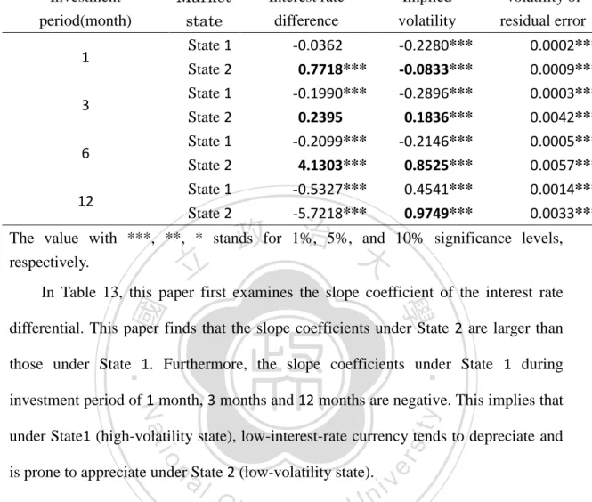
(45) 5.4 The results of two-stage Markov switching model The two-stage Markov-switching model divides the whole sample into two parts ─ State 1 and State 2. State 1 is low-volatility regime and State 2 is high-volatility regime. This paper then discusses the relationship between interest rate differential, FX implied volatility and FX change. The FX quotation is units of high-interest-rate currency per low-interest-rate currency per. In our paper, JPY and CHF, USD are considered high-interest-rate currencies. AUD, NZD, MXN, REAL, ZAR, RUBEE, USD are considered low-interest-rate currencies. Due to the limited space, this paper. 政治大 paper provides the results of Markov-switching model of other currencies and related 立. only provides one example for developed market and one for developing market. This. ‧. ‧ 國. 學. graphs in Appendix I to Appendix VI.. er. io. sit. y. Nat. al. v. n. Table 11 The results of two-stage Markov switching model of NZDUSD for different investment periods Investment period(month) 1 3 6 12. Ch. Market state State 1 State 2 State 1 State 2 State 1 State 2 State 1 State 2. engchi. i Un. Interest rate difference. Implied volatility. Volatility of residual error. 1.0078*** 1.4867*** 1.7401***. -0.3522*** -0.0153 -0.5873***. 0.0005*** 0.0009*** 0.0013***. 3.5835*** -3.1259*** 7.9120*** -0.6604*** 12.1744***. -0.2836*** 1.1079*** -1.1719*** 0.3803*** -2.2889***. 0.0017*** 0.0013*** 0.0059*** 0.0018*** 0.0079***. The value with ***, **, * stands for 1%, 5%, and 10% significance levels, respectively. 45.