具撓性腱腱驅動機構動力模式之研究

行政院國家科學委員會專題研究計畫 成果報告

具撓性腱腱驅動機構動力模式之研究

計畫類別： 個別型計畫

計畫編號： NSC92-2218-E-002-038-

執行期間： 92 年 08 月 01 日至 93 年 07 月 31 日

執行單位： 國立臺灣大學機械工程學系暨研究所

計畫主持人： 李志中

計畫參與人員： 顏宏哲, 孫緯翰

報告類型： 精簡報告

處理方式： 本計畫可公開查詢

中 華 民 國 93 年 8 月 19 日

行政院國家科學委員會補助專題研究計畫

_成果報告

具撓性腱腱驅動機構動力模式之研究

計畫類別：■ 個別型計畫 □ 整合型計畫

計畫編號：NSC 92－2218－E －002 －038－

執行期間： 92 年 8 月 1 日至 93 年 7 月 31 日

計畫主持人：李志中

共同主持人：

計畫參與人員： 孫緯翰、顏宏哲

成果報告類型(依經費核定清單規定繳交)：■精簡報告 □完整

報告

本成果報告包括以下應繳交之附件：

□赴國外出差或研習心得報告一份

□赴大陸地區出差或研習心得報告一份

□出席國際學術會議心得報告及發表之論文各一份

□國際合作研究計畫國外研究報告書一份

處理方式：除產學合作研究計畫、提升產業技術及人才培育研究計

畫、列管計畫及下列情形者外，得立即公開查詢

□涉及專利或其他智慧財產權，□一年□二年後可公開查

詢

執行單位：

國立台灣大學 機械工程學系

中

華 民 國 93 年 8 月 10 日

Abstract

In this paper, a systematic methodology for the dynamic analysis of tendon-driven robotic mechanisms with compliant tendons is presented. The compliance of tendons and inertias of the intermediate links in the mechanism are taken into account. Representing the tendon force by use of a rectifying operator, the unidirectional force transmission

characteristic of tendons can be preserved. The dynamic equations can then be systematically established in a recursive manner using the Newton-Euler equations. The joint reaction forces and the tension in each segment of tendon can be also obtained. The methodology can be applied to both endless and open-ended tendon-driven robotic mechanisms.

Keywords: dynamic analysis, tendon-driven, compliance, recursive, Newton-Euler equations

Introduction

For decades, the robotic manipulators using tendon transmission have attracted

researchers for applications in many areas such as the design of dexterous mechanical hands [1, 2], parallel cable-suspended manipulators [3, 4], teleoperating robots, etc. A unique characteristic associated with robotic manipulators using tendons drive lies in that tendons can only exert tension, i.e., force is only transmitted in a unidirectional sense. As a result, it increases the complexity in the control of such mechanical systems. The problem can be further complicated by friction and compliance embedded in the tendons and/or inertia of the extra components used in the systems. Therefore, it would be useful to research on the development of an analytical model that can account for a number of their realistic properties, such as tendon compliance, link inertia, and/or joint friction in order to produce predictions that are important for design. Also, it can provide the means for the engineer to realize the performance of such mechanical systems for future extent.

A number of analytic modeling methods for tendon-driven systems have been proposed and studied. The kinematics and statics of articulated tendon-driven robotic mechanisms have been investigated by Morecki et al. [5], Salisbury [1] and Tsai and Lee [6]. Ideal tendons with no compliance were used in their studies. Hollars and Cannon [7] experimented on the control of a two-link manipulator with flexible tendons. They concluded that the flexibility in drive

trains has a significant influence on the fine position control of tendon-driven systems. Chang [8] used the stiffness constant to represent the stiffness of tendons and studied the compliance of tendon-driven robotic mechanisms. Prisco and Bergamasco [9] derived the dynamics of a type (2N) of multi-degree-of-freedom tendon-driven manipulators, which is the structure that Utah-MIT hand [2] belongs to. On the other hand, there is also literature investigating on the performance of single-DOF tendon devices [10, 11] of which the kinematic structure is less coupled than that of multi-DOF systems.

In this paper, a systematic methodology for generating the dynamic model of robotic mechanisms with compliant tendons is presented. A model is first developed for representing the unidirectional force transmission characteristic of tendons. The resulting representation is then combined with the Newton-Euler algorithm to generate the system dynamic equations. The procedure is shown by the application of the method to a two-linked tendon-driven robotic manipulator and a one-DOF manipulator equipped with a simple servo-control. The results show that the unique characteristic of tendon transmission can be preserved in the modeling. Also, it shows that the modeling will be degraded if the compliance associated with position control is not properly managed.

Assumptions

In [6], some general assumptions about the structural characteristics have been

introduced for the kinematic and static analysis of tendon-driven manipulators. To adapt to the scope of dynamic analysis, the following assumptions for tendon-driven manipulators are considered.

（Ⅰ）All tendons are under tension. The amount of stretch in tendon is small and linearly proportional to the tendon force.

（Ⅱ）No slippage occurs between pulleys and tendons.

（Ⅲ）Tendons are lightweight such that the weight/inertia, flexural bending, and shear effects of tendons will not be considered.

parts of the transmission are not included. Nevertheless, these terms may be added in the modeling where the force control is important.

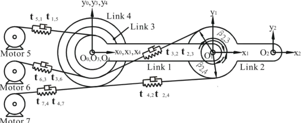
Tendon drives can generally be classified into two types of routing [6, 12] as: (1) the open-ended type and (2) the endless type of routing. In the open-ended tendon routing, as shown in Fig. (1a), one end of the tendon is fixed to a moving link to be controlled while the other end is attached to a driving actuator. From the moving link to the driving actuator, each tendon routing forms a transmission line. A unique characteristic of such open-ended tendon drives is that tendons transmit the forces in a unidirectional sense. On the other hand, the routing of the endless tendons is shown in Fig. (1b) in which two pulleys of constant center distance are wrapped around by an endless tendon. The driven pulley is attached to a link to be controlled and the driving pulley is installed on a rotary actuator or fixed to a driven pulley of prior pulley train stage. From the driven link to the driving actuator, the tendon-and-pulley also forms a transmission line. In an endless tendon drive, the pulley can be driven in both directions. One side of the tendon will be under higher tension while the other side is under lower tension.

It can be noted that after the removal of tendons and intermediate/idle pulleys, the tendon-driven robotic mechanism becomes a serial type open-loop chain. We call the links that constitute the open-loop chain as the primary links, and all other links as the intermediate links. An intermediate link is said to be carried by a primary link i if it is connected to link i by a revolute joint. As shown in Fig. (1a), link 0, 1, 2 and 3 are the primary links, and link 4, 5 are the intermediate links. Intermediate link 4 and 5 are carried by the primary link 1.

Kinematics of Primary Links

To facilitate the analysis, each primary link from the base to the distal link is sequentially numbered from 0 to n. Meanwhile, a local coordinate system (xi, yi, zi) is

attached to the distal joint of link i according to the Denavit and Hartenberg (D-H) convention [13]. Let θi,i-1 be the joint angle from xi-1 axis to xi axis, ai,i-1 and αi,i-1 the offset distance and the twist angle between zi-1 and zi axes, and di,i-1 the translational distance measured from xi-1 axis to xi axis along zi-1 axis. Then, the matrix transforming the ith coordinate to (i-1)th

coordinate can be written as i-1_A

i = (1)

where Cθi,i-1 =Cos(θi,i-1), Sθi,i-1=Sin(θi,i-1), Cαi,i-1=Cos(αi,i-1), Sαi,i-1 =Sin(αi,i-1).

The velocities and accelerations of the primary links can be derived from the forward recursive method [14], computing from the proximal moving link toward the end-effector link, as ) ( i1 _i1 1 i , i 1 i 1 i 1 i i i i − − − − − − +θ = R ω z ω & (2) ) ( i1 1 i 1 i, i 1 i 1 i 1 i 1 i 1 i, i 1 i 1 i 1 i i i i − − − − − − − − − − − +θ + ×θ = R ω z ω z

ω& & && & (3)

1 1 1 1− − − − + × = i _ii i i i i i i i i , p ω v R v (4) ) ( ii,1 i i i i i 1 i 1 i 1 i i 1 i, i i i i i i − − − − − + + × × × =ω p R v ω ω p

v& & & (5)

) ( ic i i i i i i i ic i i i ic i r ω ω v r ω

v& = & × + & + × × (6)

where ωi is the angular velocity vector of link i, vi is the velocity vector of the origin Oi, vic is the velocity of the center of mass of link i, ric is position vector defined from the mass center of link i to Oi, i-1zi-1=[0, 0, 1]T is a unit vector defined along zi-1 axis, iRi-1 is the transpose of the upper left 3×3 sub-matrix of i-1_A

i, and ipi,i-1 is the vector as

i_p

i,i-1=[a i,i-1, d i,i-1Sαi,i-1, d i,i-1Cαi,i-1]T (7)

Kinematics of Intermediate Links

A local coordinate system (xj, yj, zj) is defined for each intermediate link according to the D-H convention. Consider an intermediate link j located on the primary link i, the

            − − − − − − − − − − − − − − − − − − − 1 0 0 0 d C S 0 S a C S C C S C a S S S C C 1 i i 1 i i 1 i i 1 i i 1 i i 1 i i 1 i i 1 i i 1 i i 1 i i 1 i i 1 i i 1 i i 1 i i 1 i i 1 i i 1 i i , , , , , , , , , , , , , , , , , α α θ θ α θ α θ θ θ α θ α θ

coordinate transformation matrix from the jth coordinate system to the ith coordinate is given by             α α θ θ α − θ α θ θ θ α θ α − θ = 1 0 0 0 d C S 0 S a C S C C S C a S S S C C i, j i, j i, j i, j i, j i, j i, j i, j i, j i, j i, j i, j i, j i, j i, j i, j j i i , j B (8)

Suppose links i, j, and k are coaxial. Then, the relative motion among these links can be related by the coaxial condition as

k ,j j , i k , i =θ +θ θ (9)

The velocity and acceleration of intermediate link j can be also obtained by modifying Eqs. (2)~(6) as j j i, j i i i j j j_{ω = Q ω +θ& z (10)} j j i, j i i i j j j i, j i i i j j

j_{ω& = Q ω& +θ&& z + Q ω ×θ& z (11)}

i, j j j j i i i j j j_{v = Q v + ω× p (12)} ) p ω ( ω Q v Q p ω vj j j j j,i j ii i j ii i j j j j,i j _{= × + + × ×} & & & (13) )] ( [ ) ( jc j i, j j i i i j i i i j i i i j jc j i, j j i i i j jc j r p ω Q ω Q v Q r p ω Q v + × × + + + × = & & & ₍₁₄₎ where j_Q

i is the transpose of the upper left 3×3 sub-matrix of iBj, rjc is the position vector defined from mass center of links j to Oj, and jpj,i can be written as

j_p

Modeling of Unidirectional Force in Tendon

A number of models for the dynamics of tendon-driven robotic manipulators with elastic tendons have been developed [7, 8, 15]. In the models, the elastic tendon connecting two pulleys is represented by a linear spring. Since linear springs can exert tensile as well as compressive force, therefore, modeling the tendon with linear spring will inevitably be biased from the realistic characteristics of tendon. In this work, a method for modeling the

unidirectional force in the tendon is proposed. The method utilizes the rectifying concept that was used by Jacobsen et al. [2] and Lee and Tsai [16]. Jacobsen et al. ever used a rectifying operator to transform the joint torque space into tendon force (or motor torque) space for the Utah-MIT dexterous hand. Lee and Tsai further extended the concept to motor torque analysis for the n×(n+1) tendon-driven systems. In what follows, the basic principle of such concept will be first introduced. Then, the procedure of the application for the tendon force analysis will be developed. Let the operator O+(x) be defined as







<

≥

=

+

0

x

,

0

0

x

,

x

)

x

(

O

(16)

where x is a dummy variable. The function of O+_{(x) can be plotted graphically as shown in} Fig. 2. Also, O+_{(x) can be written as}

2

)

x

x

(

)

x

(

O

+

=

+

₍₁₇₎

It can be noted that O+_{(x) returns its value only when the argument is positive.} Otherwise, O+_{(x) gives zero value.}

Figure 3 shows the planar schematic of a simple tendon-and-pulley pair, where link k is the carrier and links i and j are the two pulleys. Pulley i and j are coupled by a flexible tendon having the spring constant ki,j and damping coefficient ci,j. If the positive rotation of pulley is defined as the pulley rotates counter clockwise, then, for small angular rotations of the pulleys, the magnitude of tendon force, ti,j, can be written as

[

t

k

(

r

θ

r

θ

)

c

(

r

θ

r

θ

)

]

O

t

_i,j

=

+ _0i,,j

−

_{i,j i i,k}

−

_{j ,jk}

−

_{i,j i}

& −

_{i,k j}

&

_,jk (18a)

where t0,i,j is the amount of pretension that is initially set in the tendon. The physical meaning of Eq. (18a) can be readily seen from Fig. 3. If the value in the square bracket is greater than zero, then the tendon is under tension and the operator returns the value. On the other hand, if the value in the square bracket is less than zero, ti,j is equal to zero and the tendon is slack. Therefore, the equation implies that the tendon force can be transmitted only when the relative displacement between two pulleys causes tendon under tension. In general, to satisfy different types of pair connections, Eq. (18a) can be rewritten as

[

0i,,j i,j i i,k i,j j ,jk i,j i i,k i,j j ,jk

]

j

i,

O

t

k

r

θ

k

r

θ

c

r

θ

c

r

θ

t

=

+

±

±

±

& ±

&

(18b)

where the ± sign of each term is to be determined by the tendon routing topology. The sign is positive if the pulley tends to pull tendon from the other end; otherwise, it is negative.

Tendon Forces Analysis

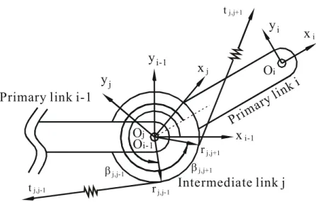
Since each transmission line begins from the primary link and ends at the link driven by the rotary actuator, the tendon may route through one or more intermediate links. Consider the intermediate link j on the distal joint of a primary link i-1 as shown in Fig. 4. Let the carrier of the pulley pair (j, j+1) be the primary link i, and the carrier of the pulley pair (j, j-1) be the primary link i-1. Also, let the portion of the tendon connecting intermediate links j and j+1 be

tj,j+1, and the other portion connecting links j and j-1 be tj,j-1.

For a general tendon-pulley pair, the tendon will engage with the pulley at a constant direction with respect to the carrier. In addition, for the pulley to run in both directions, the direction of tendon acting on the pulley should be tangential to the pitch circle of the pulley plane. As shown in Fig. 4, define the radius vector rj,j+1 of tendon tj,j+1 as the vector from the axis of rotation to the tangent point and wrapping angle βj,j+1 as the angle measured from the x-axis of coordinate system on link i to the radius vector in a right-hand rule direction. Note that in spatial case, the x-axis is defined by the coordinate systems of the pulley j and link i

according to the D-H method. Similarly, radius vector, rj,j-1, and the wrapping angle, βj,j-1, for tendon tj,j-1 can be defined in the (i-1)th system. The radii vectors and tendon forces are summarized as

[

]

T 1 i, j 1 j,j j 1 j,j j 1 i i 1 j ,j i

_r

_C

_r

_S

_b

+ + + − +

= G

⋅

β

β

r

(19a)

[

]

T 1 i, j 1 j,j j 1 j,j j 1 j ,j 1 i

_r

_C

_r

_S

_b

− − − − −

_r

₌

_β

_β

_(19b) 1 j ,j i 1 j ,j 1 j ,j i _t + + + = u t (20a) 1 j ,j 1 i 1 j ,j 1 j ,j 1 i _t − − − − − _{t = u (20b)}

where rj is the radius of link j, bj,i+1 is the distance measured from origin Oi to the center of pulley j along zj, bj,i-1 is the distance measured from origin Oi-1 to the center of pulley j along zj-1, tj,j+1 and tj,j-1 are respectively the magnitudes of tj,j+1 and tj,j-1, which can be formulated form Eq. (18b). Vectors i_u

j,j+1 and i-1uj,j-1 are respectively the unit vectors of itj,j+1 and i-1tj,j-1 and can be written as

[

]

T 1 j,j 1 j,j 1 i i 1 j ,j i

_S

_C

₀

+ + − +

= G

⋅

−

β

+

β

u

(20c)

[

]

T 1 j,j 1 j,j 1 j ,j 1 i

_S

_C

₀

− − − −

_u

₌

₊

_β

₋

_β

_(20d)

The transformation matrix i_G

i-1 is defined as:

          α α − α α = − − − − − 1 i, i 1 i, i 1 i, i 1 i, i 1 i i C S 0 S C 0 0 0 1 G (21)

The tendon forces can be transformed to the jth coordinate system on link j by multiplying a suitable rotational matrix j_R

i-1. 1 j ,j i i j 1 j ,j j + + = R t t (22a) 1 j ,j 1 i 1 i j 1 j ,j j − − − − = R t t (22b) Dynamic Analysis

For a given mechanism, the force and moments exerted by different links on each other can be determined via Newton and Euler’s equations. While solving the dynamics using Newton and Euler’s equations, three force- and three moment-balance equations can be established for each link of the mechanism. To solve the simultaneous equations in an efficient way, rather than solving all the unknowns simultaneously, one tries to solve them in a recursive manner. The joint forces will first be expressed in the state of motions, and then the state of motions will be obtained by solving the differential equations. After the state of motions is solved, the joint forces can then be determined by back substituting the tendon forces into the balance equations.

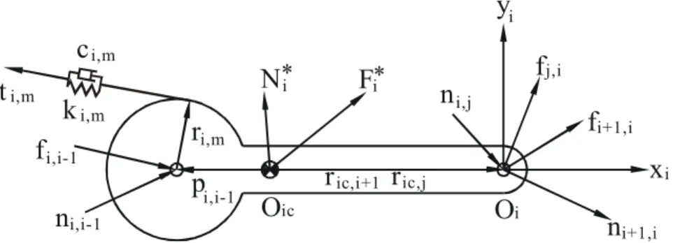
Dynamics of Primary Links

Fig. 5 shows the free body diagram of a primary link i which connects to link (i-1) at joint (i-1) and link (i+1) at joint i. Assume that primary link i is driven by an mth tendon or more. The force and moment balance equations for link i can be represented in the following recursive forms:

∑

∑

− ± ± ± ± + + = − − − − + + − j i, j i m , i i 1 i, m m i,m 1 i,i i i,m 1 i, m m i,m 1 i,i i i,m m , i, 0 m 1 i, i i 1 i, i i * i i ) θ r c θ r c θ r k θ r k (t O f u f f F & & (23a) and

] ) θ r c θ r c θ r k θ r k (t O ) [( ) ( m , i i 1 i, m m m , i 1 i,i i m , i 1 i, m m m , i 1 i,i i m , i m , i, 0 m ic i m , i i j j i, j i j , ic i j , i i 1 i, i i 1 i, ic i 1 i, i i ic i 1 i, i i 1 i, i i * i i u p r f r n f r f p n n N − − − − + + + − + − ± ± ± ± × + + × − + × + × + + =

∑

∑

∑

& & (23b) where i_u

i,m is the unit vector of ti,m acting on link i. The vector iui,m can be determined from Eq. (20c,d). i_F

i* and iNi* are the inertia force and moment vectors of primary link i, and can be obtained as: ic i i * i i_{F m v} & = (24a)

(

c ii i

)

i i i i i c * i i

_N

₌

_I

_ω

_&

₊

_ω

_×

_I

_ω

_(24b)

where mi is the mass of link i, and c_{Ii is the inertia tensor of link i with respect to a center of} mass coordinate system, which has the same orientation as the ith coordinate system.

The vector terms in Eqs. (23a) and (23b), fi+1,i and ni+1,i, are computed from the balance equations of the preceding link while fj,i and nj,i are the forces and moments from intermediate links. For the end-effector link, these vectors represent the end-effector output force and moment. The other unknown terms: fi,i-1, ni,i-1, θi,i-1 and θm,i-1 always constitute more than six scalar unknowns. Hence they cannot be solved one link at a time.

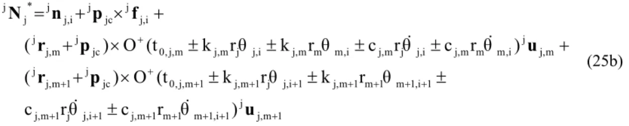
Dynamics of Intermediate Links

Referring to Fig. 6 the intermediate link j is located on link i, the force and moment balance equations for an intermediate link j can be written as

1 m ,j j 1 i, 1 m 1 m 1 m ,j 1 i, j j 1 m ,j 1 i, 1 m 1 m 1 m ,j 1 i, j j 1 m ,j 1 m ,j , 0 m ,j j i, m m m ,j i, j j m ,j i, m m m ,j i, j j m ,j m ,j , 0 i, j j * j j ) θ r c θ r c θ r k θ r k (t O ) θ r c θ r c θ r k θ r k (t O + + + + + + + + + + + + + + + + ± ± ± ± + ± ± ± ± + = u u f F & & & & (25a)

and 1 m ,j j 1 i, 1 m 1 m 1 m ,j 1 i, j j 1 m ,j 1 i, 1 m 1 m 1 m ,j 1 i, j j 1 m ,j 1 m ,j , 0 jc j 1 m ,j j m ,j j i, m m m ,j i, j j m ,j i, m m m ,j i, j j m ,j m ,j , 0 jc j m ,j j i, j j jc j i, j j * j j

)

θ

r

c

θ

r

c

θ

r

k

θ

r

k

(t

O

)

(

)

θ

r

c

θ

r

c

θ

r

k

θ

r

k

(t

O

)

(

+ + + + + + + + + + + + + + + + +

±

±

±

±

×

+

+

±

±

±

±

×

+

+

×

+

=

u

p

r

u

p

r

f

p

n

N

&

&

&

&

(25b) where j_u

j,m and juj,m+1 are the unit vectors of tj,m and tj,m+1 acting on link j, and can be determined from Eq. (20c, d). j_F

j* and jNj* are the inertia force and moment of link j, and can be computed similarly by Eq. (24a) and (24b).

The tendon force tj,j+1 in Eq.(25a) & (25b) can be computed form the moment balance equation of the upper level intermediate link. Once the joint forces and the moment of upper level links are solved, the unknown forces and moments in Eq. (25a) and (25b) can be solved associated with the unknown forces and moments in the primary link. We also note that any vector defined in its local coordinate system on the intermediate link can be related to the coordinate system of its corresponding primary link by Eqs. (19), (20), and (22).

We have derived the basic equations, which are required for the dynamic analysis of articulated, tendon-driven robotic mechanisms. The derivation of dynamic equations of the articulated, tendon-driven robotic devices will be described. Two examples will be used for illustration.

Examples

Example 1. A Robotic manipulator driven by flexible tendons

Fig. 7 shows a two-jointed, four-link robotic manipulator driven by three open-ended tendons. The tendons are spooled to the motors located at the base link 0. In this system, each segment of tendon between two rigid links is flexible with certain spring constant and

damping coefficient. The vectors required for the kinematics are summarized in Table 1, while the vectors for the tendon forces are in Table 2 and 3.

(23a), (23b), (25a) and (25b) as Link 2 * 2 4 , 2 3 , 2 1 , 2

t

t

F

f

+

+

=

(26a) * 2 4 , 2 c 2 4 , 2 3 , 2 c 2 3 , 2 1 , 2 c 2

f

(

r

p

)

t

(

r

p

)

t

N

p

×

+

+

×

+

+

×

=

(26b) Link 3 * 3 6 , 3 2 , 3 0 , 3

t

t

F

f

+

+

=

(26c) * 3 6 , 3 c 3 6 , 3 2 , 3 c 3 2 , 3 0 , 3 c 3

f

(

r

p

)

t

(

r

p

)

t

N

p

×

+

+

×

+

+

×

=

(26d) Link 4 * 4 7 , 4 2 , 4 0 , 4

t

t

F

f

+

+

=

(26e) * 4 7 , 4 c 4 7 , 4 2 , 4 c 4 2 , 4 0 , 4 c 4

f

(

r

p

)

t

(

r

p

)

t

N

p

×

+

+

×

+

+

×

=

(26f) Link 1 1 , 2 * 1 5 , 1 0 , 1

t

F

f

f

+

=

+

(26g) 1 , 2 2 , c 1 * 1 5 , 1 c 1 5 , 1 0 , 1 c 1

f

(

r

p

)

t

N

r

f

p

×

+

+

×

=

+

×

(26h)

Expressing the force f2,1 in Eq. (26a) in terms of tendon forces and substituting into Eq. (26b), the moment balance equation of link 2 could be obtained as:

))]} ( ) ( ( ) ( [ ))] ( ( )) ( ( [ { )] )( ( ) ( )[ ( ) ( , , , , , , , , , , , , , , , , , , , , , , , , , , , , , , 0 4 0 1 3 2 0 4 0 1 4 2 4 1 2 3 2 1 2 4 2 2 4 2 0 0 3 0 1 3 1 2 2 3 2 0 3 0 1 3 1 2 2 3 2 3 2 0 2 1 2 0 1 2 2 0 1 1 2 2 0 1 1 2 1 2 2 2 1 2 0 1 2 c k r c k r t O r r c r r k t O r s a C S a s a m I θ θ θ θ θ θ θ θ θ θ θ θ θ θ θ θ θ θ θ θ & & & & & & && && && & && && − + − + + + − − − − − − − + + − + + − − = + + + ₍₂₇₎

Similarly, the moment balance equations of links 3, 4, and 1 could be respectively obtained as: )]} r r ( c ) r r ( k t [ O ))] ( r r ( c )) ( r r ( k t [ O { r I 0 , 6 6 0 , 3 3 6 , 3 0 , 6 6 0 , 3 3 6 , 3 6 , 3 , 0 0 , 3 0 , 1 3 1 , 2 2 2 , 3 0 , 3 0 , 1 3 1 , 2 2 2 , 3 2 , 3 , 0 3 0 , 3 3 θ + θ + θ + θ + − θ − θ − θ − θ − θ − θ − = θ + + & & & & & && (28) )]} ( ) ( [ ))] ( ( )) ( ( [ { , , , , , , , , , , , , , , , , , , , 0 7 7 0 4 4 7 4 0 7 7 0 4 4 7 4 7 4 0 0 4 0 1 4 1 2 2 2 4 0 4 0 1 4 1 2 2 2 4 2 4 0 4 0 4 4 r r c r r k t O r r c r r k t O r I θ θ θ θ θ θ θ θ θ θ θ & & & & & && + + + + − − + + − + + = + + (29) )]} ( ) ( )[ ( { ) ( )] ( ) ( [ ))] ( ( )) ( ( [ ) ( ))] ( ( )) ( ( [ ) ( , , , , , , , , , , , , , , , , , , , , , , , , , , , , , , , , , , , , , , 1 2 0 1 1 2 2 1 2 0 1 1 2 2 2 2 0 1 1 1 1 0 1 2 1 1 0 1 2 1 2 1 0 5 5 0 1 1 5 1 0 5 5 0 1 1 5 1 5 1 0 1 0 4 0 1 4 1 2 2 4 2 0 4 0 1 4 1 2 2 4 2 4 2 0 4 2 0 3 0 1 3 1 2 2 3 2 0 3 0 1 3 1 2 2 3 2 3 2 0 3 2 0 1 1 C S s a m s m 2 a s m m m a r r c r r k t O r r r c r r k t O r r r r c r r k t O r r I θ θ θ θ θ θ θ θ θ θ θ θ θ θ θ θ θ θ θ θ θ θ θ θ θ θ && && & & && && && & & & & & & & & && + − + − + + − + − + − + + − + + − + + − + + − + − − − − − − + − = + + + (30)

Equations (27)~(30) are the equations of motion of the system. One the equations of motion are solved, the tension in each segment of tendon can be calculated via the equations in Table 2.

Example 2. Control of the one-DOF manipulator driven by two actuators

In this example, a one-DOF device is used to demonstrate the difference in control performance with and without O+ _{operator acting on the tendons. As shown in Fig. 8, the} one-DOF manipulator is driven by two flexible tendons spooled to the actuators on the ground. A simple “ PD feedback” control technique is implemented for controlling the manipulator. Following the same procedure illustrated in Example 1, the dynamic equation can be concluded as:

)] ( ) ( )] ( ) ( , , , , , , , , , , , , , 0 2 2 0 3 3 2 3 0 2 2 0 , 3 3 2 , 3 2 3 0 3 0 1 1 0 3 3 1 3 0 1 1 0 , 3 3 1 , 3 1 3 0 3 0 3 3 θ r θ r C θ r θ r K [T O r θ r θ r C θ r θ r K [T O r I & & & & && − − − − + − + − + − = + + θ (31)

and the inputs are designed as

)

(

K

)

(

K

_{P d 3,0 D d 3,0} 0 , 1

=

θ

−

θ

+

θ

−

θ

θ

&

&

(32)

)

(

K

)

(

K

_{P d 3,0 D d 3,0} 0 , 2

=

θ

−

θ

+

θ

−

θ

θ

&

&

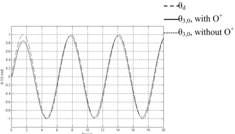
(33)

Figure 9 shows the block diagram of the control system. The designed output of θ3,0 is a sinusoidal function Sin(t). The dynamic system is simulated and the results are shown as follows.

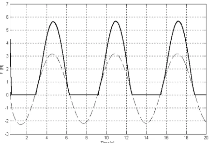
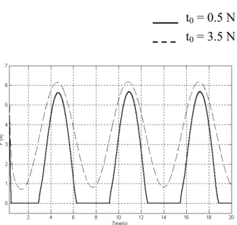
Figure 10 shows the motion responses of the output with and without the rectifier O+ _in the dynamic equation. The results of the outputs will depend on the stiffness of tendon as well as the proportional and derivative gains tuned for the controller. The higher the stiffness of tendons is, the more similar outputs of the two models become. The tendon force in each tendon is also plotted in Fig. 11a and 11b where the pretension t0 is set to 0.5N. It can be seen that negative values appears in the tendon force curves for the system without the rectifier O+ in the equation. This result does not comply with the force transmission characteristics of tendons. Thus, if the tendon force is required in force control method, there may cause errors for the results.

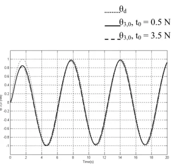
To compare the performance of the system under different pretension, the system is simulated with t0 = 0.5 N and 3.5 N. Fig. 12 shows the motion response of the output while Fig. 13a and 13b show the responses of tension in tendons. Comparing the tendon force curves shown in Fig. 13a and 13b. It can be noted that the higher the pretension is, the stiffer the system is. Also, note that the tendons with t0 = 0.5N reached zero tension state during the operation. Thus, it can be concluded that if pretensioning is not well managed, system modeling may cause slackness in tendons and results in errors. Therefore, the pretension of

tendons may play an important role in the dynamic response of tendon-driven manipulators.

Conclusion

A systematic methodology for the dynamic analysis of tendon-driven robotic

mechanisms with flexible tendons is developed. A novel representation of the tendon force is introduced. The O+ _{operator is used to represent the force transmission characteristics of} tendons. The method subsequently uses the recursive algorithm to calculate the dynamics of links. Tendon forces, reaction forces and compliance effects are all derived by the methods developed in this research.

The performance of such system is also studied by implementing a PD controller onto a one-DOF system. The results of the system output with and without the operator in the equation are compared. It is also shown that the magnitude of pretension of tendons may play an important role in the dynamic response of tendon-driven manipulators.

References

1. J. K. Salisbury, Kinematic and Force Analysis of Articulated Hands, Ph.D. Dissertation, Dept. of Mechanical Engineering, Stanford University, Stanford, CA, 1982.

2. S.C. Jacobsen, J.E. Wood, D.F. Knutti and K.B. Biggers, "The Utah-MIT Dexterous Hand: Work in Progress," The Int'l J. of Robotics Research, Vol. 3, No. 4, 1985, pp.21-50.

3. J. Albus, R. Bostelman and N. Dagalakis, "The NIST Spider, A Robot Crane," J. Res. NIST, Vol.97, No.3, 1992, pp.373-385.

4. S. Kawamura, W. Choe, S. Tanaka, and S.R. Pandian, "Development of an Ultrahigh Speed Robot FALCON using Wire Drive System," IEEE Int'l Conf. On Robotics and Automation, 1995, pp.215-220.

5. A. Morecki, Z. Busko, H. Gasztold and, K. Jaworek, Synthesis and Control of the Anthropomorphic Two-Handed Manipulator, Proc. of the 10th _{Int'l Symposium on Industrial Robots, Milan, Italy,} 1980, pp. 461-474.

6. L. W. Tsai and J. J. Lee, "Kinematic Analysis of Tendon-Driven Robotic Mechanisms Using Graph Theory," ASME J. Mechanisms, Transmissions, and Automation in Design, Vol. 111, No. 1, 1989, pp. 59-65.

Manipulator with Flexible Tendons," ASME Winter Annual Meeting, Miami, FL, 1985. 8. S. L. Chang, 1993, “Compliance and Dynamic Analysis of Tendon-Driven Robotic

Mechanisms,” ASME, Proceedings of the 19th Annual ASME Design Automation Conference. Part 1 (of 2), Sep 19-22 1993, Albuquerque, NM, USA, pp. 229-233.

9. G.M. Prisco and M. Bergamasco, “Dynamic Modeling of a Class of Tendon Driven Manipulators,” Proc IEEE Int'l Conf Robotics Automat, Monterey, CA, July 7-9, 1997.

10. S. C. Jacobsen, H. Ko, E. K. Iversen, and C. C. Davis, Antagonistic Control of a Tendon-Driven Manipulator, Proc. IEEE Int'l Conf. Robotics Automat, 1989.

11. C. R. Johnstun and C.C. Smith, Modeling and Design of a Mechanical Tendon Actuation Systems, ASME J. Dynamic Systems, Measurement, and Control, Vol. 114, 1992, pp. 253.

12. L. W. Tsai, Robot Analysis-The mechanics of Serial and Parallel Manipulators, John Wiley & Sons, Inc., 1999.

13. J. Denavit and R. S. Hartenberg, A Kinematic Notation for Lower Pair Mechanisms Based on Matrices, ASME J. Applied Mechanics, Vol.77, 1955, pp. 215-221.

14. D.E. Orin, R.B. McGhee, M. Vukobratovic, and G. Hartoch, Kinamatic and Kinetic Analysis of Open-Chain Linkage Utilizing Newton-Euler Methods, Math. Biosci., Vol. 43, 1979, pp. 107-130. 15. M. Kaneko, W. Pactsch, and H. Tolle, "Input-Dependent Stability of Joint Torque Control of Tendon

Driven Robot Hands," IEEE Trans. On Industrial Electronics, Vol.39 (2), 1992.

16. J. J. Lee and L. W. Tsai, Torque Resolver Design for Tendon-Driven Manipulators, ASME J. Mechanical Design, Vol. 115, No. 4, 1993, pp. 877-883.

Nomenclature

j i

c_, : The damping ratio of the tendon connecting link i and j j

i

k_, : Stiffness of the tendon connecting link i and j

* F_i i

: Inertia force of link i with respect to frame i

1 i i i − ,

f

: Force acting on link i by link i-1 at joint i

* N_i

i _{: Inertia moment of link i with respect to frame i}

1 i i i − ,

n

: Moment acting on link i by link i-1 at joint i

i

1 i i i − ,

p

: Position vector defined from O_i-1 to O_i

ic i_p

: Position vector defined from mass center of link i to joint i

1 i i

−

R : Rotation matrix, which transforms (i-1)th coordinate system to ith coordinate system

ic i

_r

: Position vector defined from Oi to the mass center of link i

1 i ic i + ,

r

: Position vector defined from the mass center of link i to joint i+1

j ic i

,

r

: Position vector defined from the mass center of link i to joint j

k i i

,

r

: Position vector defined from joint i to the mesh point of the tendon

k i i

,

t

: The kth tendon-force acting on link i with respect to frame i

m i 0

t

_,, : Pretension of mth tendon acting on link I

i i

_v

: Velocity of the origin O_i

ic i

_v

: Velocity of the center of mass of link i

m i,

u : Unit vector of mth tendon acting on link i

k j,

β : Wrapping angle of link j mounted on pulley-pair (j, k)

1 i i,−

θ : Angular displacement between link i and link i-1

i i

_ω

Fig.1a

Open-ended type tendon routing

θ

j,k

θ

j,k

.

θ

i,k

θ

i,k

.

k

_i

j

+

k

i,j

c

i,j

Fig. 3

A parallel-type routing pulley pair

Intermediate link j

tj,j+1 tj,j-1

y

_i-1

x

i-1

O

i-1

O

j

Primary link i-1

βj,j+1 βj,j-1 rj,j+1 rj,j-1

x

j

y

_j

x

i

y

_i

Pri

ma

ry

lin

k i

O

i

Fig. 4 A typical intermediate link j carried by a primary link i-1

1

1

O

+

(X)

X

0

Fig. 2

Function of O+_(x)

F

i*

N

*i

t

i,m

f

i,i-1

n

i,i-1

n

_i+1,i

f

i+1,i

x

i

y

_i

O

i

O

ic

r

i,m

p

_i,i-1

r

ic,i+1

f

j,i

n

_i,j

r

ic,j

k

i,m

c

i,m

Fig. 5

A typical primary link i

F

*

j N_j*

_t

_j,m+1

t

j,m

f

j,i

n

j,i

O

jc

r

_j,m+1

r

_j,m

p

_jc

O

_j

O

i

k

j,m

c

j,m

k

j,m+1

c

_j,m+1

x

_j

y

_j

t2,3 t3,2 Link 2 y1 x1 x0,x3,x4 y0,y3,y4 O0,O3,O4 Link 1 Link 4 Link 3 β 2,4 β 2,3 O1 x2 y2 O2 t 2,4 t 4,2 t1,5 t3,6 t4,7 t5,1 t6,3 t7,4 Motor 5 Motor 6 Motor 7

Fig. 7a A robotic manipulator driven by flexible tendons

y1 x1 x0,x3,x4 y0,y3,y4 O0,O3,O4 O1 x2 y2 O2 s1 s2 a1 a2

Fig. 7b

Kinematics of Figure7a

1

2

3

0

t

_3,1

t

_3,2

θ

_3,0

θ

1,0

θ

2,0

PD controller

Plant

+

−

θ

3,0

θ

d

Fig. 9

Block diagram of the PD control 0 , 3 0 , 3

,θ

θ

&

Fig. 10

Comparison of θ3,0 with and without O+

θ

d

θ

3,0

, with O

+

θ

3,0

, without O

+

Fig. 11a Comparison of tendon force t3,1 with and without O+

Fig. 11b Comparison of tendon force t3,2 with and without O+

with O

+

without O

+

with O

+

without O

+

Fig. 12 Responses of θ3,0 under different pretensions

θ

d

θ

3,0

, t

0

= 0.5 N

θ

3,0

, t

0

= 3.5 N

Fig. 13 Responses of t3,1 with different pretensions

Fig. 14 Responses of t3,2 with different pretensions

t

0

= 0.5 N

t

0

= 3.5 N

t

0

= 0.5 N

t

0

= 3.5 N

Table 1 Kinematics of the robotic mechanism in Example 1 1

_P

1c

=[-(a

1

-s

1

), 0, 0]

T

,

2

P

2c

=[-(a

2

-s

2

), 0, 0]

T

,

3

P

3c

=[0, 0, 0]

T

[

]

T 0 , 1 1 1

_ω

₀

₀

_θ

_&&

& =

,

[

]

T 0 , 1 1 1 2 0 , 1 1 1 c 1 1

_v

₍

_s

_a

₎

_θ

&

₍

_a

_s

₎

_θ

&&

₀

&

=

−

−

[

]

T 1 , 2 0 , 1 2 2

_ω

₀

₀

_θ

&&

_θ

&&

&

=

+

,





















+

−

+

+

+

−

+

+

−

=

0

)

)(

s

a

(

S

a

C

a

)

)(

a

s

(

S

a

C

a

v

2 _{2 2 1,0 2,1} 0 , 1 1 , 2 1 0 , 1 1 , 2 1 2 1 , 2 0 , 1 2 2 0 , 1 1 , 2 1 2 0 , 1 1 , 2 1 c 2 1

_θ

_θ

_θ

_θ

_θ

_θ

θ

θ

θ

θ

θ

θ

&&

&&

&

&&

&

&

&&

&

&

[

]

T 0 , 3 3 3

_ω

₀

₀

_θ

_&&

& =

,

3

_v

_3c

₌

[

₀

₀

₀

]

T

&

[

]

T 0 , 4 4 4

_ω

₀

₀

_θ

_&&

& =

,

4

_v

_4c

₌

[

₀

₀

₀

]

T

&

Table 2 The magnitudes of tendon forces for Example 1 )] ( ) ( _{, , , ,} , ,23 2,3 2 2,1 3 31 23 2 21 3 31 0 2,3 O [t k rθ rθ c rθ rθ t = + − + − & + & )] ( ) ( _{, , , ,} , ,24 2,4 2 2,1 4 41 24 2 21 4 41 0 2,4 O [t k rθ rθ c rθ rθ t = + + − + & − & )] ( ) ( , , , , , ,32 3,2 2 21 3 3,1 32 2 21 3 31 0 3,2 O [t k rθ rθ c rθ rθ t = + − + − & + & )] ( ) ( _{, , , , ,} , ,36 3,6 3 30 6 60 36 3 30 6 60 0 3,6 O [t k rθ rθ c rθ rθ t = + + + + & + & )] ( ) ( _{, , , ,} , ,42 4,2 2 21 4 4,1 42 2 21 4 41 0 4,2 O [t k rθ rθ c rθ rθ t = + + − + & − & )] ( ) ( _{, , , , ,} , ,47 4,7 4 40 7 70 47 4 40 7 70 0 4,7 O [t k rθ rθ c rθ rθ t = + + + + & + & )] ( ) ( _{, , , , ,} , ,15 1,5 1 10 5 50 15 1 10 5 50 0 1,5 O [t k rθ rθ c rθ rθ t = + − − − & − &

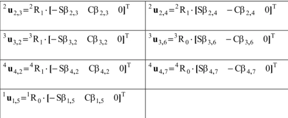
Table 3 The unit vectors of tendon forces for Example 1 T 3 2 3 2 1 2 3 2 2_{u R [ S C 0]} , , , = ⋅ − β β 2u2,4=2R1⋅[Sβ2,4 −Cβ2,4 0]T T 2 3 2 3 1 3 2 3 3_{u R [ S C 0]} , , , = ⋅ − β β 3u3,6=3R0⋅[Sβ3,6 −Cβ3,6 0]T T 2 4 2 4 1 4 2 4 4_{u R [ S C 0]} , , , = ⋅ − β β 4u4,7=4R0⋅[Sβ4,7 −Cβ4,7 0]T T 5 1 5 1 0 1 5 1 1_{u R [ S C 0]} , , , = ⋅ − β β