A Fast Mixed Integer Programming Formulation for the Maximum Set Covers Problem in Wireless Sensor Networks

A Fast Mixed Integer Programming Formulation for the Maximum

Set Covers Problem in Wireless Sensor Networks

Pi-Rong Sheu

1, 2

, Ming-Yen Lin

2

, Meng-Hao Liu

1

, and Chen-Fong Huang

1 1

_{Department of Electrical Engineering, National Yunlin University of Science and}

Technology, Touliu, Yunlin 640, Taiwan, R.O.C.

2

_{Institute of Communications Engineering, National Yunlin University of Science and}

Technology, Touliu, Yunlin 640, Taiwan, R.O.C.

Email: sheupr@yuntech.edu.tw

Abstract

-In a wireless sensor network

(WSNET), the target coverage (TC) problem is to schedule the activity of each sensor such that each target is monitored by some sensor at every moment and the network lifetime is maximized. A possible approach to deal with the TC problem is to organize all the sensors into a group of non-disjoint sets such that each set can completely monitor all the targets within a certain time interval and only one set is active at any time instant. This approach is known as the maximum set covers (MSC) problem, which has been proven to be NP-complete. In this paper, the MSC problem is studied. There has existed a mixed integer programming formulation (MIPF) for the MSC problem, named as MIPF-for-MSC, which can find its optimal solution. However, the execution time of MIPF-for-MSC is heavy. In this paper, we design a preprocessing technique and a new inequality to speed up the execution of MIPF-for-MSC. Computer simulations show that compared with the original MIPF-for-MSC, our preprocessing technique and new inequality can reduce the execution time significantly. Keywords: integer programming, maximum set cover, power-saving, target coverage, wireless sensor network.

1. Introduction

A WSNET is formed by a large number of tiny sensing devices (or called sensors) [10] [12]. A sensor in a WSNET can generate as well as forward data, which are gathered from every sensor’s vicinity and will be delivered to the single remote base station (or called the sink). Two sensors in such a network can communicate directly with each other through a single-hop routing path in the shared wireless media if their positions are close enough. Otherwise, they need a multi-hop routing path to carry out their

communications. In a multi-hop routing path, the data packets sent by a source sensor are relayed by several intermediate sensors before reaching the sink. WSNETs are useful in a broad range of environmental sensing applications such as vehicle tracking, seismic data, and so on.

Since WSNETs are characterized by their limited battery-supplied power, the network lifetime is restricted at the battery power and the speed of power-consumption of each sensor. Extensive research efforts have been devoted to the design of power-saving mechanisms such that the total power consumption in a WSNET is minimized and the network lifetime is maximized. In this paper, the lifetime of a WSNET is defined to be the time period from the beginning of the network operation to when one of the targets can not be monitored. A possible power-saving mechanism is to schedule each sensor to alternate its states between the active and sleep mode. This is because while some requirements are met, compared with another case of each sensor being active continuously, the case of each sensor altering its states between the active and sleep mode will generate a longer network lifetime [1-3].

One of the most important design issues in a WSNET is the TC problem [2]. In the TC problem, targets are located in known locations. Given a WSNET consisted of sensors, where these sensors are randomly distributed near by these targets such that a sensor can monitor one or some targets, the TC problem is to schedule the activity of each sensor such that each target is monitored by at least one sensor at every moment and the network lifetime is maximized. The TC problem has attracted a lot of attention recently [1-3]. In particular, a possible approach to deal with the TC problem is to organize all the sensors into a group of non-disjoint sets such that each set can completely monitor all the targets during a

m

n m

certain time interval and only one set is active at any time instant. In other words, these sensor sets in this group are activated successively. At any time instance, each sensor belonging to the active set is in its active state while all the other sensors are in the sleep state. This approach is known as the MSC problem, which has been proven to be NP-complete [2].

In this paper, the MSC problem is studied. Mixed integer linear programming formulations (MILPFs) [7] have been adopted by many researchers to solve various problems in wireless networks [4-6] [11]. Similarly, there has existed a mixed integer programming formulation (MIPF) for the MSC problem, named as MIPF-for-MSC, which can find its optimal solution [2]. However, the execution However, the execution time of MIPF-for-MSC is very long. Several efficient schemes have been proposed to speed up the execution of a MIPF [9]. For example, a preprocessing technique can be applied to the given input before the execution of a MIPF. Another efficient scheme is to add more inequalities to the original MIPF. In this paper, an efficient preprocessing technique and an efficient inequality are proposed to speed up the execution of MIPF-for-MSC (i.e., to speed up the finding of solutions to the MSC problem). Simulation results show that compared with the original MIPF-for-MSC, our preprocessing technique and new inequality can reduce the execution time significantly.

The rest of the paper is organized as follows. In Section 2, a formal definition of the MSC problem is given. In Section 3, the existing MIPF-for-MSC is presented. In Section 4, an efficient preprocessing technique and an efficient inequality for the MIPF-for-MSC are proposed. In Section 5, the performance of the proposed preprocessing technique and inequality is evaluated through computer simulations and compared to that of the original MIPF-for-MSC. Lastly, Section 6 concludes the whole research.

2. Problem Definition

In this section, some assumptions and notations for the MSC problem are given first. Then, the MSC problem is defined formally and explained in detail [2].

Assumptions and Notations for the MSC Problem [2]

The following states some important assumptions and notations used in the MSC problem considered in this paper.

(1) Every sensor has the same sensing range. The sensing range of a sensor is centralized in itself. It may monitor all the targets within the area of its sensing radius. (2) Every sensor has the same battery power.

The lifetime of every sensor is defined to be

one time unit.

(3) If the sensing range of a sensor is larger than the distance between itself and a target, then the sensor can monitor the target. If a target is out of the sensing range of a sensor, then the target can not be monitored by the sensor.

(4) The state of a sensor is either active or sleep.

(5) There are m targets to be monitored. There are n sensors

1, 2, , m

r r r

v v " v

1, 2, , n

s s

v v " _s in a WSNET. These sensors

are randomly deployed to monitor all the targets. That is, each target is required to be always monitored by at least one sensor at any time.

v

Definition of the MSC Problem

In a given WSNET, all the targets must be monitored by one or more sensors at any time. A group of sensors is called a cover set if all the targets in the WSNET can be monitored by the sensors in during a time interval of length . The parameter is named as the time weight associated with . For a given group of cover sets

k S , k S k t t_k { k | k S k 1, 2, } U = S = " p , the

calculation of each tk is as follows. Let

{

k1, sk2, vsk

}

S = v v " ,

n

k s . If there are x cover

sets each of which includes

ki s v , then the lifetime of ki s v is 1 k i s v x Λ = . Thus, mi _ki ki n s k s k = v S t v ∧ ∈ .

Now the MSC problem is defined formally as follows. Given a WSNET consisting of a set of targets { | 1, 2, , } j r R= v j= " m { | 1, 2, , } i s C= v i= " n { k| 1, 2, , U S k and a set of sensors , find a group of cover sets = = " p} k S p t in which every cover set has a time weight such that the summation of time weights,

= k t T t₁+ +t₂ "+ k t

, is maximized, where the value of in

[ ]

0,1

,Sp

1 2

. To be more specific, the MSC problem is to find a group of cover sets such that all the targets are continually monitored by each cover set during a time interval of length and the network lifetime 1, ,2 S S " k S k t p t + +t "+t is maximized. As an illustration of the above notations and definitions, let us consider the following example. Figures 1 and 2 show an instance of the MSC problem. Figure 1(a) shows a WSNET consisting of three sensors vs₁,vs₂,vs₃ and three

targets v vr₁, r₂,vr₃. All of the three sensors 3 1, 2, s s v v v_s i

have the same sensing radius. Figure 1(b) represents the relationship between the sensors and the targets in Figure 1(a). An arrow from a sensor v to a target s denotes that

target j r v j r

v can be monitored by sensor i

s

v . For

example, there exist an arrow between targets 1 s v 2 r v

and / . This indicates that targets and can be monitored by sensor

1 r v v_r2 v_r1 1 s v . S i mi l a r l y, ta rg e ts a n d c a n b e monitored by sensor 2 r v 2 3 r v s v . Targets and

can be monitored by sensor

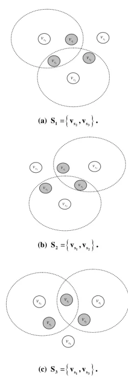
1 r v 3 r v 3 s v . Figure 2 shows a group of possible cover sets for the MSC problem defined by Figure 1. Figure 2(a) shows that all the three targets can be m o n i t o r e d b y s e n s o r s 1 2 r r v v 2 3 , , v_r s v a n d v s₃

simultaneously during the first time interval of length . That is, S v . Similarly, Figure 2(b) shows that all the targets can be

1

t 1=

{

s₂,vs₃

}

monitored by sensors vs₁ and v s2 simultaneously during the second time interval of length t₂, i.e., S₂ =

{

v_s1,v_s2

}

. Finally, Figure 2(c) shows S

{

v_s1,v_s3

}

3 t 1 S S2 3= 3 , ,vr

during the third time interval of length . To sum up, all the three targets can be completely monitored by the sensors in , , and , respectively, during three different time intervals.

1 2

r r

v v

3

S

As each sensor is used to monitor the targets twice in the three different time intervals

1 s v 2 s v 3 s v 1 r v 2 r v 3 r v

{

2 3

}

1 s s (a) S = v , v

.

1 s v 2 s v 3 s v 1 r v 2 r v 3 r v target ensor s 1 s v 2 s v 3 s v 1 r v 2 r v 3 r v

{

1 2

}

2 s s (b) S = v , v

.

(a) A WSNET. 1 s v 2 s v 3 s v vr1 2 r v 3 r v

{

1 3

}

3 s s (c) S = v , v

.

1 s

v

2 s

v

3 s

v

1 r

v

2 r

v

3 r

v

(b) The relationship of coverage between sensors and targets.

Figure 2. A group of possible cover sets for the MSC problem in Figure 1.

(i.e., each sensor appears twice in the three different cover sets, , ), the time weight of each cover set is . Thus, the network lifetime of the WSNET given in Figure 1 is . j S 3 1.5 t = 1, 2,3 j= i S i t 0.5 1 2 t + +t

3. An existing MIPF for the MSC

problem

In this section, an existing MIPF for the MSC problem, named as MIPF-for-MSC, proposed in [2] is presented.

Network Model

A WSNET is represented by a finite set of

sensors and a set of

targets . A set of

is used to describe the relationship between sensors and targets. That is, if sensor

{ | 1, 2, , } i s C= v i= " n { | 1, 2, , j r R= v j= " m

k sensor v monitors targes

i } t

{

i k

}

C = i | v_r s v k C

can monitor target , then i is put into .

k

r

v

A Known MIPF for optimally solving the MSC problem: MIPF-for-MSC

The variables used in MIPF-for-MSC are defined in the following.x : a binary variable, ij

where and . Its

value is 1 when sensor

1, 2, , i= " n j=1, 2,",p i s Sj v ∈ j t and 0 otherwise, where is a cover set. : the time weight of cover set

j

S

j

S , where . Its value is between 0 and 1.

1, 2,

j= ", p

Thus, MIPF-for-MSC can be described as follows: Maximize: 1 2 p t + t + " + t (1) Subject to: 1 1 p ij j j x t = ≤

∑

for all (2) i s v ∈C 1 k ij i C x ∈ ≥

∑

for all , 1, 2, , (3) k r v ∈R j= " p ij x =0 or 1, = 1 if and only if i ij s j x v ∈S (4)

The objective function (1) is used to maximize the network lifetime. The inequality (2) states that the total time interval scheduled for each sensor in all set covers is not larger than 1, which is the lifetime of each sensor. Inequality (3) guarantees that every target is monitored by at least one sensor

k r v i s v in every

cover set . Inequality (4) expresses the integrality of variable

j

S

ij

x

4. Our Efficient Preprocessing

this section, we propose an ef

Technique and Inequality

In ficient

pre

explain the ide

processing technique and a new inequality to speed up the execution of MIPF-for-MSC.

Our Preprocessing Technique

First, let us use an example to

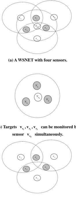
a behind our preprocessing technique. Consider Figure 3(a). The locations of all the three targets are within the sensing radius of sensor v_s4. Thus, sensor

4

s

v can monitor

targets vr₂，vr3 simultaneously, as shown by Figure 3(b). Therefore, it is feasible to schedule sensor ₄

1

r

v ，

s

v to monitor all the targets by

itself in a single t e interval. Figure 3(c) shows im

1 r v 3 s v 3 r v 2 s v 2 r v 1 s v 4 s v

(a) A WSNET with four sensors.

1 r v 3 r v vr2 4 s v

(b) Targets can be monitored

1 2 3 r r r v , v , v or 4 s v sim by sens ultaneously.

1 s v 2 s v 3 s v 1 r v 2 r v 3 r v

(c) The simplified WSNET.

Figur our

preprocessing technique.

esultant WSNET after sensor vs₄ is dele

Figure 3(c) is the same as Fig

the r ted.

si

e deleted from the WSNET before the

nd our new e. Consider Figure 4. Tar

Obviously, ure 1.

In other words, Figure 3(a) can be mplified to become Figure 1 before the MIPF-for-MSC is applied to it.

Based on the observation, our idea is that a sensor may b

execution of the MIPF-for-MSC if it can monitor all the targets by itself in a single time interval. The computer simulations in Section 5 show that such deletions, i.e., such a preprocessing technique, can indeed speed up the execution of MIPF-for-MSC.

Our New Inequality

First, let us explain the idea behi inequality via an exampl

get 1

r

v can be monitored by at most two

sensors: vs₁ and vs3 . Target vr3 can be monitored by at most two sensors: v_s2 and v_s3.

Target vr₂ can be monitored by a ost th

sensors ₁

t m ree : vs , vs2, and vs4. Thus, it is not hard to discove k lifetime of of the WSNET in Fi e 4 ca ot exceed 2. In other words, the network lifetime

p

r that the netw n nor gur 1 j j= sens es t

∑

of a WSNET is dominated by minimum Tc

can monitor a certain target. As a r ult, we have a new inequality

p

the among the maxim m nuu ers of

1

mb ors which

j c

t ≤T

∑

. In Figure 4, it canbe observed is equal to 2. Hence,

2

j

t ≤

∑

. Furt ore, if there exist

j= c T rm that 1 p j= he Ms

ch of which can monitor all the targ

sensors ea ets

in the WSNET by itself, then our new inequality

1 s v 2 s v 3 s v 1 r v 2 r v 3 r v 4 s v

Figure 4. An example to illustrate our new inequality (9). can be rewritten as p s j M t 1 c T = j ≤

∑

≤ .

Obviously, we must calculate the values of

s

M and _c for a given WSNET before our

inequality can be applied. Our computer lations show that the time to find the values of

T

new simu

s

M and T_c is very short.

Now, our new MIPF for the MSC problem, named as NM PF-for-MSC canI be described as follows: Maximize: t1 + t2 + " + tp (5) Subject to: 1 1 ij j j x t = p ≤

∑

for i s v ∈C all (6) 1 k ij i C x ∈ ≥

∑

for all v , 1, ,p k r ∈R j= " (7) ij x = 0 or 1, xij = 1 if and only if vsi ∈Sj (8) 1 p s j c j M t T = ≤

∑

≤ (9)

Simulations

In this section, we examine the efficiency of ew inequality thr sen simulations there ions are sho

5. Computer

our preprocessing technique and n

ough computer simulations. Our performance comparisons are conducted among the three different formulations: (1) The original MIPF for the MSC problem: MIPF-for-MSC, which consists of inequalities (1) to (4). (2) Our new MIPF for the MSC problem: NMIPF-for-MSC, which consists of inequalities (5) to (9). (3) Our NMIPF-for-MSC + our preprocessing technique. The three formulations are solved by the LINGO 8.0 software package [8] run at a typical personal computer consisted of Intel Core 2 Duo 2.13 GHz and 1G MB DDRII SDRAM. The execution time of each formulation is observed.

Our computer simulations are carried out on a number of WSNETs generated randomly. The

sors and targets are randomly located on a grid of 500m × 500m. Every sensor has the same sensing radius, which is set to 250m . Our computer consider two different cases. In case 1, it is assumed that exist sensors which can monitor all the targets by itself at the same time. There do not exist such sensors in case 2. In other words, only case 1 has cover sets consisting of a single sensor.

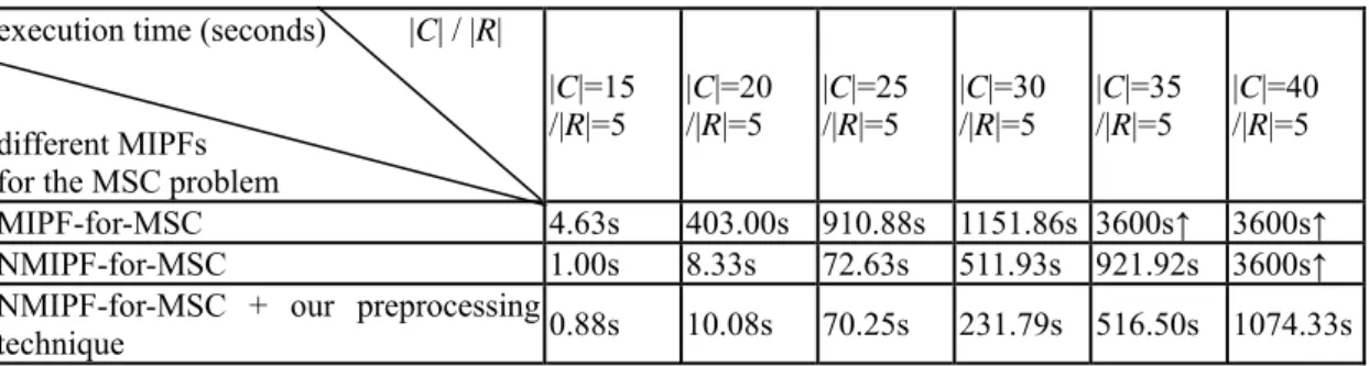
For case 1, the execution times required by each of the three different formulat

wn in Table 1, where 3600s↑ denotes that the execution time exceeds 3600 seconds. Table 1 shows that compared with MIPF-for-MSC, our NMIPF-for-MSC is able to shorten the execution

times from (4.63 1.00) 4.63 78.40%− = to (1151.86 511.93) 1151.86 55.56%− = when the network size is from C =15 / R =5 to

30 / 5

C = R = . M our

NMIPF-for-MSC + our preprocessing technique execution times from

oreover, can shorten the

(4.63 0.88) 4.63 80.99%− = to (1151.86 231.79) 1151.86 79.88%− = when the network size is from C =15 / R = to 5

30 / 5

C = R = . To sum up, t es

of our NMIPF-for-MSC and our + our preprocessing technique are clearly much less than that of MIPF-for-MSC.

For case 2, the simulation results are shown in Table 2. Compa

he execution tim NMIPF-for-MSC

red with MIPF-for-MSC, our NMIPF-for-MSC can shorten the execution time up to (44.82 25.73) 44.82 42.59%− = and

(616.70 156.55) 616.70 74.61%− = when the network size is C =20 / R =5 and

25 / 5

C = R = , respectively

that our new inequality is able to shorten the n most cases.

6. Conclusions

. It can be observed execution time i

In this paper, we ha studied the MSC Ts. The MSC problem has bee

Acknowledgement

ported in part by the Nat

eferences

W. Lou, M. Li, and X. Li,

[2] Li, and W. Wu,

[3] and M. O. Pervaiz,

Table 1. The execution times of different MIPFs ith WSNETs including single-sensor cover sets.

t MIPFs with WSNETs without single-sensor cover sets. C|=15 |C|=20 |C|=25 |C|=30 |C|=35 |C|=40 ve

problem in WSNE

n proven to be NP-complete and a MIPF for its optimal solutions has been proposed. However, the existing MIPF has a heavy execution time. This makes the finding of the optimal solutions of the MSC problem impractical in most situations. In this paper, we

have designed an efficient preprocessing technique and an efficient inequality to speed up the execution of the existing MIPF. The computer simulations verify that compared with the original MIPF, our preprocessing technique and inequality can reduce the execution time in most cases. In particular, when there exist sensors which can monitor all the targets in the WSNET by itself at the same time, the reduction is significant.

This work was sup

ional Science Council of the Republic of China under Grant No. NSC 96-2221-E-224-005-MY2.

R

[1] Y. Cai,

"Target-Oriented Scheduling in Directional Sensor Networks," Proceedings of the 26th IEEE International Conference on Computer Communications (IEEE INFOCOM 2007), pp. 1550-1558, May 2007.

M. Cardei, M. T. Thai, Y.

"Energy-Efficient Target Coverage in Wireless Sensor Networks," Proceedings of the 24th Annual Joint Conference of the IEEE Computer and Communications Societies (IEEE INFOCOM 2005), Vol. 3, pp. 1976-1984, March 2005.

M. Cardei, J. Wu, M. Lu,

"Maximum Network Lifetime in Wireless Sensor Networks with Adjustable Sensing Ranges," Proceedings of the IEEE International Conference on Wireless and

w execution time (seconds) |C| / |R|

Table 2. The execution times of differen _| diffe t MIPFs

em ren

for the MSC probl

/|R|=5 /|R|=5 /|R|=5 /|R|=5 /|R|=5 /|R|=5 MIPF-for-MSC 4.63s 403.00s 910.88s 1151.86s 3600s↑ 3600s↑

NMIPF-for-MSC 1.00s 8.33s 72.63s 511.93s 921.92s 3600s↑ NMIPF-for-MSC + our preprocessing

technique 0.88s 10.08s 70.25s 231.79s 516.50s 1074.33s

execution time (seconds) |C| / |R| different MIPFs

for the MSC problem

|C|=15

/|R|=5 |C|=20 /|R|=5 |C|=25 /|R|=5 |C|=30 /|R|=5 |C|=35 /|R|=5 |C|=40 /|R|=5 MIPF-for-MSC 0.90s 44.82s 616.70s 330.65s 3600s↑ 3600s↑ NMIPF-for-MSC 1.75s 25.73s 156.55s 423.40s 825.10s 3600s↑

Mobile Computing, Networking and 3, pp. J. Marks, M. El-Shark

. Gray, “Minimum power for wireless networks:

integer formulati

Proceedi Second A

Joint Confere EE Computer and Communications Societies (IEEE INFOCOM 2003), vol. 2, 2003, pp. 1001-1010.

[5] A. K. Das, R. J. Marks, M. A. El-Sharkawi, P. Arabshahi, and A. Gray, “Optimization Methods for Minimum Power Multicasting in Wireless Networks with Sectored Antennas,” Proc. of IEEE Wireless Communications and Networking Conference, March 2004, pp. 1299-1304. [6] S. Guo and O. W. Yang, “Minimum-Energy

Multicast Routing in Static Wireless Ad Hoc Networks,” Proc. of IEEE International Conference on Network Protocols (ICNP'04), vol. 6, September 2004, pp. 3989-3993.

[7] F. S. Hillier and G. J. Lieberman, Introduction to Mathematical Programming,

n G l,

htt .li /.

[9] R. Montemanni and L. M. Gambardella, “Exact Algorithms for the Minimum Power

ym iv b n

ir e d

vo no .

2891-2904, November 2005.

[10] C. S. R. Murthy and B. S. Manoj, Ad Hoc Wireless Networks: Architectures and Protocols, Prentice Hall,2004.

[11] C. Wang, M. T. Thai, Y. Li, F. Wang, and W. Wu, “Minimum Coverage Breach and Maximum Network Lifetime in Wireless Sensor Networks,” Global Telecommunications Conference (IEEE GLOBECOM 2007), pp. 1118-1123, November 2007.

[12] F. Zhao and L. Guibas, Wireless Sensor Networks: An Information Processing Approach, Morgan Kaufmann, San Francisco, 2004.

Communications (WiMob 2005), Vol. 438-445, August 2005. [4] A. K. Das, R. awi, P. Arabshahi, and A broadcast trees programming ons,” ngs of the Twenty-nce of the IE nnual 2 d ed., Mc raw-Hil 1995. [8] p://www ndo.com

S metric Connect ity Pro lem i W Oper eless N ations Re etworks,” search, Comput l. 32, rs an.11, pp