Cascaded Class Reduction for Time-Efficient Multi-Class Classification

全文

(1)Int. Computer Symposium, Dec. 15-17, 2004, Taipei, Taiwan.. Cascaded Class Reduction for Time-Efficient Multi-Class Classification∗ Jyh-Jong Tsay Ching-Han Lin Chi-Wei Hung Chi-Hsiang Lin. Department of Computer Science and Information Engineering National Chung Cheng University Chiayi, Taiwan 62107, ROC. Abstract. studied in areas such as data mining, machine learning and statistics, and arises in wide variety of applications such as, for example, text categorization, web page classification, classification of biological sequences, image recognition, speech recognition, and mining of business data, to name a few. These applications often involve hundreds or thousands of classes.. Classification of objects into a fixed number of predefined categories has been extensively studied in wide variety of applications such as, for example, text categorization, web page classification, classification of biological sequences, image recognition, speech recognition, and mining of business data, to name a few. These applications often involve hundreds or thousands of classes. Experiments show that approaches such as SVM and KNN often outperform other approaches, but suffer long classification time especially when the number of classes involved is large. In this paper, we investigate and propose a cascaded class reduction method in which a sequence of classifiers are cascaded to successively reducing the set of possible classes. We show that by cascading SVM and KNN with time-efficient classifiers such as linear classifiers and naive Bayes, we can significantly reduce the classification time of SVM and KNN while maintaining and sometimes improving their classification accuracy. Keywords. Classification, KNN, Multiple Classifier System, SVM, Text Categorization. A large number of approaches [6, 7, 8] have been proposed for classification such as, for example, linear classifiers, decision trees, naive Bayes, k-nearest neighbors(KNN), neural networks, and support vector machines(SVM), to name a few. It has been reported [10] that simple classifiers such as linear classifiers and naive Bayes are very time-efficient in both training and classification stages. On the other hand, SVM [8, 12] and KNN [15] outperform simple classifiers in classification accuracy, especially when the number of classes involved is very large, for example, in the categorization of web pages into directories maintained by information portals such as Google and Yahoo. One of the common disadvantages of KNN and SVM in such applications is that they both require long classification time. One of the interesting question that we may ask is as follows: Can we combine the strengths of timeefficient classifiers such as linear classifiers and naive Bayes, and top performers such as SVM and KNN so that the running time of SVM and KNN can be reduced while their accuracy is maintained? To study and answer the question, we propose a cascaded class reduction (CCR) approach in which a sequence of classifiers are cascaded to successively reduce the set of possible classes. Observe that in applications such as text. 1 Introduction Classification is defined as the task of automatic assignment of input objects into a fixed number of predefined categories. This problem has been extensively ∗ This research is supported in part by the National Science Council, Taiwan, ROC, under grant NSC-93-2213-E-194-021.. 1 189.

(2) Int. Computer Symposium, Dec. 15-17, 2004, Taipei, Taiwan.. of positive and negative examples. In this paper, we choose α = 0.5. Widraw-Hoff (WH) is another algorithm to produced linear classifiers. WH is an online algorithm. It runs through the training examples one at a time, updating a weight vector at each step. Initially, the weight vector is set to the all zero vector, i.e. w1 = (0,...,0). At each step, the new weight vector wi+1 is computed from the old weight vector wi using training examples xi with label yi . The jth component wi+1,j of the new weight vector is computed as follows.. categorization, linear classifiers and naive Bayes often achieve excellent performance in top r measure for small r such as 3 or 4. Namely, the target class is one of the first r classes ranked by them. In CCR, SVM and KNN are used to determine the final prediction from the first r classes ranked by linear classifiers and naive Bayes. Experiment on data sets collected from web directories shows that our approaches significantly reduce the running time of SVM and KNN while maintaining and sometimes improving their classification accuracy. For example, on the data set collected from Yahoo directory, the classification time of SVM is reduced from 50.26 sec to 13.88 sec for classifying 4,177 test instances, while the classification accuracy is slightly improved from 0.764 to 0.767. The remainder of this paper is organized as follows. Section 2 reviews basic classifiers used in this paper. Section 3 presents cascaded class reduction. Section 4 gives experimental results. Section 5 concludes.. ωi+1,j = ωi,j − 2η(ωi · xi − yi )xi,j where η > 0 is the learning rate which controls how quickly the weight vector ω is allowed to changed, and how much influence each new example has on it. Note that label yi = 1 if xi is a positive example, and yi = 0 if xi is negative. We set η = 1/(4l2 ) where l is the maximum value of ||xi || in the training set. The final prototype vector g is the the average of the weight vectors computed along the way.. 2 Basic Classifiers In this section, we briefly review the classifiers which are used later in this paper. We assume that we are given N training examples (x1 , y1 ), . . . , (xN , yN ), where yi denotes the label of xi and xi = (xi,1 , xi,2 , . . . , xi,d ) is a d-dimensional vector . Rocchio (ROCC) is a batch algorithm for training linear classifiers. In linear classifier[6], one prototype vector is computed for each class. To classify an instance x, we compute the cosine similarity between x and every prototype. The label of the prototype whose similarity to x is maximum is assigned to x. There are several algorithms such as Rocchio and Widrow-Hoff proposed to produce linear classifiers. The prototype of a class computed by ROCC is the centroid of positive examples, tuned by negative examples. Let E+ denote the set of positive examples, i.e. the set of examples in that class, and E− denote the set of negative examples, i.e. the set of examples in other classes. ROCC computes the prototype vector g as follows. P. g=. x∈E+. |E+ |. x. P. −α. x∈E−. g=. X 1 n+1 ωi n + 1 i=1. Naive Bayes (NB) classifier is a simplified version of Bayesian classifiers widely used in many applications. The basic idea in NB is to use the joint probabilities of terms and classes to estimate the probabilities of classes given a document. The naive part of NB is the assumption of terms independence, i.e., the conditional probability of a term given a class is assumed to be independent from the conditional probabilities of other words given that class. Let v be a class and x be an instance. NB assign the class v to x that maximizes P (v|x) which is estimated as follows. P (v) P (x|v)P (v) = P (v|x) = P (x). Q. T F (ti ,x) ti ∈x P (ti |v). P (x). where ti is a term appearing in x, and T F (ti , x) is the term frequency of ti in x. K-Nearest Neighbor(KNN) [15] is a lazy learning algorithm that simply stores all training examples in memory, and doesn’t need training phase. To classify a new instance x, KNN finds the k nearest neighbors of x in the training set by calculating the cosine similarity. x. |E− |. where α is a parameter to adjust the relative impact 2. 190. ,.

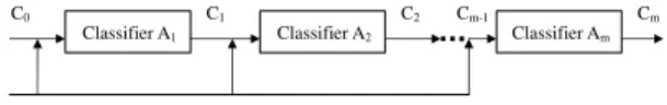
(3) Int. Computer Symposium, Dec. 15-17, 2004, Taipei, Taiwan.. between x and every training examples. The similarity score of each of the k neighboring examples when it compared to x is used as the weight of the class of the neighboring example. The sum of the class weights over the k nearest neighbors is used to perform class ranking. The class with the highest score is assigned to x. In our experiment, we choose k = 15. Given a training set of labelled examples, Support Vector Machine(SVM) [11] constructs a hyperplane that maximizes the margin between the sets of two classes (positive and negative). The SVM decision function is of the form,. C0. C1 Classifier A1. C2. Cm. Cm-1. Classifier A2. Classifier Am. Figure 1. Cascaded Class Reduction. We have experimented other types of kernels, and the results are similar. In this paper, we use LIBSVM [1] developed by Chang and Lin for the experiment.. 3 Cascaded Class Reduction. f (x) = sign((w · x) + b). The main idea is to cascade a sequence of classifiers A1 , A2 , . . . , Am as in Figure 1. Let Ci denote the output, for example a ranked list, produced by classifier Ai . In classification stage, Ai takes as input the instance x and the output Ci−1 produced by Ai−1 , and produces output Ci . Ci is then passed to Ai+1 as part of its input. In general, Ci can be generalized to contain any information produced by Ai . Several Multiple Classifiers Systems(MCS) [3, 9] can be translated to above framework. For example, in voting by a committee, Ai appends its prediction to Ci−1 to form Ci , and Am simply perform voting, using votes stored in Cm−1 . In this paper, we propose Cascaded Class Reduction (CCR) in which Ai identifies a set Ci of most possible classes from classes in Ci−1 received from Ai−1 . We assume classes in each Ci are ranked. We apply CCR to combine classifiers which are simple but achieve very high top r measure such as linear classifiers and naive Bayes, and classifiers which achieve top classification accuracy but take long classification time such as KNN and SVM. Our objective is to reduce the classification time of SVM and KNN while maintaining similar classification accuracy.. where w is a vector determining the orientation of the plane, and b is the offset from the origin. The function implies that an instance x is assigned to the positive class if w · x + b > 0; otherwise, it is assigned to the negative class. The optimal solution for a training set is found by determining w and b such that: 1 min kwk2 , yi (w · xi − b) ≥ 1 2 Since the margin between two classes is defined as by minimizing 12 kwk2 , the margin between the two classes will be maximized. When the data is not linearly separable, we try to simultaneously maximize the margin and minimize the classification error as follows. 2 , kwk2. n X 1 ²i , yi (w·xi −b) ≥ 1−²i , ²i ≥ 0 min kwk2 +C 2 i=1. In this paper, we choose C = 1. Another approach to handle nonlinear separable case is to map each instance x to a vector Φ(x) in the feature space. Notice that to compute the dot product of Φ(xi ) and Φ(xj ) in the feature space, a kernel function is defined as follows.. 3.1 Cascaded SVM We apply CCR to to combine simple classifiers and SVM. Figure 2 gives the pseudo code for WH-SVM in which WH and SVM are cascaded. On receiving an instance x, WH-SVM first invokes WH which in turns, computes the cosine similarity between x and the prototype vector of each class, and returns a list of classes sorted by the computed similarity values. WH-SVM. K(xi , xj ) = hΦ(xi ) · Φ(xj )i There are several well-known kernels such as linear kernels, polynomial kernels((1 + xi · xj )k ), and RBF kernels(exp(−kxi − xj k2 /σ 2 )). The experimental result listed in this paper is obtained from linear kernels. 3. 191.

(4) Int. Computer Symposium, Dec. 15-17, 2004, Taipei, Taiwan. Size of Size of Number Data Source WH-SVM(x, r, threshold) Testing Set Training Set of classes 5,004 36,148 12 CNA RankedList = WH(x); 4,391 10,059 95 Openfind 4,177 10,029 99 Yahoo Candidates = top r classes in RankedList; FinalClass = SVM(Candidates, x); If the score of FinalClass is less than threshold, Figure 3. Statistics of Data Sets then FinalClass = the top 1 class in RankedList; Return FinalClass; and SVM. In WH-KNN-SVM, WH first produces a End of WH-SVM ranked list for KNN. KNN then re-ranks the top r1 classes received from WH. Finally, SVM determines the final prediction, considering only the top r2 (r2 ≤ Figure 2. Cascading WH and SVM r1 ) classes ranked by KNN.. then passes the top r classes ranked by WH to SVM. For each of the top r ranked classes, SVM evaluates the decision function of that class on x. SVM returns the class with the highest decision value(score). Notice that if the none of the r classes passed to SVM has score (computed by SVM) larger than a predefined threshold, WH-SVM simply takes the top 1 class ranked by WH as the final prediction. Notice that restricting the attention of SVM to solely the top r classes ranked by WH is expected to reduce the classification time of SVM as the number of classes examined by SVM is greatly reduced, as well as to improve the classification accuracy of SVM as the attention of SVM is greatly narrowed down by WH. Similar approaches are used to implement ROCCSVM and NB-SVM in which ROCC and NB, respectively, are cascaded to produce a ranked list for SVM.. 4 Experimental Results We compile the following 3 data sets, one from news collection and two from web directories. We carry out extensive experiment for cascaded SVM, cascaded KNN and WH-KNN-SVM presented in previous section. Data Set I consists of news articles collected from China News Agency(CNA), which are categorized into 12 classes. Data Set II consists of web pages in the Business category of the directory maintained by Openfind, a well-known information portal in Taiwan. The data collected from Openfind is categorized into 95 classes. Data Set III consists of web pages collected from the category Business and Economics of the directory maintained by Yahoo. The data collected from Yahoo is categorized into 99 classes. Figure 3 gives statistics of each data set. We measure the classification accuracy of each classifier, which is defined as the portion of test documents that are correctly classified. Let N denote the total number of test documents, and H be the number of test documents that are correctly classified. The classification accuracy is H N . In top k measure, a classification is counted as correct as long as the true class is one of the top k classes ranked by the classifier. Figure 4 gives the top k measure for all basic classifiers on Yahoo data. Notice that although the classification accuracy, i.e. the top 1 measure, of ROCC, NB and WH is low when compared to KNN and SVM, they achieve very high top k measure for small k, say k = 5. The classification time is the total time for the classifier to classify all test instances, staring from the first instance until all test instances are classified.. 3.2 Cascaded KNN In cascaded KNN, for example WH-KNN that cascades WH and KNN, to determine the final prediction, KNN is restricted to consider only the top r classes ranked by WH. The classification time of KNN thus can be greatly improved as all the training instances not in the top r ranked classes are ignored. We use ROCC-KNN and, resp. NB-KNN to denote the classifier in which ROCC, and resp. NB, is cascaded to KNN.. 3.3 WH-KNN-SVM We also can implement more complicated cascading such as WH-KNN-SVM that cascades WH, KNN 4. 192.

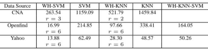
(5) Int. Computer Symposium, Dec. 15-17, 2004, Taipei, Taiwan.. ROCC NB WH KNN SVM (linear) SVM (RBF). Top 1 0.697 0.724 0.718 0.773 0.765. Top 2 0.810 0.818 0.830 0.858 0.842. Top 3 0.860 0.857 0.874 0.893 0.872. Top 4 0.886 0.882 0.901 0.907 0.888. Top 5 0.904 0.899 0.918 0.918 0.898. Top 6 0.916 0.912 0.930 0.927 0.906. 0.757. 0.853. 0.889. 0.904. 0.915. 0.922. Data Source CNA Openfind Yahoo. Openfind Yahoo. ROCC-SVM 0.775 r=3 0.634 r=4 0.756 r=6. NB-SVM 0.777 r=3 0.617 r=6 0.762 r=6. WH-SVM 0.787 r=3 0.642 r=3 0.767 r=6. SVM 1159.09 214.85 62.49. WH-KNN 521.79 r=2 97.66 r=6 28.30 r=6. KNN 1459.84. WH-KNN-SVM. 338.41. 164.05. 48.57. 50.26. Figure 6. Classification time(in sec). Figure 4. Accuracy on Yahoo Data Data Source CNA. WH-SVM 263.54 r=3 16.99 r=6 13.88 r=6. SVM 0.759. Data Source CNA. 0.576 Openfind. 0.764 Yahoo. Figure 5. Accuracy of Cascaded-SVM. ROCC-KNN 0.771 r=3 0.608 r=3 0.763 r=6. NB-KNN 0.771 r=3 0.586 r=6 0.766 r=6. WH-KNN 0.775 r=2 0.619 r=3 0.772 r=3. KNN 0.775 0.593 0.773. Figure 7. Accuracy of Cascaded-KNN. We follow the approach in [10] for preprocessing, which consists of term extraction, term selection and term clustering. In particular, we use χ2 statistics to select informative terms, and distributional clustering to cluster similar terms into term groups.. formance. The classification accuracy of WH-KNN is similar to KNN on CNA and Yahoo data, and is better than KNN on Openfind data. The classification accuracy of ROCC-KNN and NB-KNN is slightly worse than KNN, but very close. Notice that although KNN performs better than SVM, cascaded SVM performs better than cascaded KNN.. 4.1 Experiment for Cascaded SVM Figures 5 gives classification accuracy of cascaded SVM for data sets from CNA, Openfind and Yahoo. We have carried out experiment for different values of r(r = 1, 2, 3 for CNA data, and r = 1, 2 . . . , 6 for Opendfind and Yahoo data). For each data set, Figures 5 gives the best result among different values of r that we have experimented. Notice that all 3 cascaded SVM significantly improves SVM on data set from CNA and Openfind, and achieve accuracy similar to SVM on Yahoo data set. Overall, WH-SVM achieves the best performance, and consistently improves SVM on all data sets. Notice that the performance data given in Figure 5 is for SVM with linear kernels. We have performed similar experiment for SVM with RBF kernels. It is interesting to observe that although RBF kernels perform better than linear kernels in pure SVM, linear kernels beats RBF kernels when SVM is cascaded with linear classifiers. Notice that the classification time of SVM is significantly improved by WH-SVM as in Figure 6.. Notice that the classification time of KNN is significantly improved by WH-KNN as in Figure 6.. 4.3 Overall Comparison on CCR. We further compare WH-SVM, WH-KNN and WH-KNN-SVM. Figure 8 gives the classification accuracy of WH-SVM, WH-KNN and WH-KNN-SVM. It shows that WH-KNN-SVM is slightly better than WH-SVM and WH-KNN on Yahoo data, but is slightly worse than WH-SVM on Openfind data. Notice that although KNN performs better than SVM, cascaded SVM performs better than cascaded KNN. The classification time is is given in Figure 6. It shows that WH-SVM and WH-KNN significantly reduces the classification time of SVM and KNN, respectively. Overall, the experiment shows that WH-SVM that cascaded WH linear classifier and SVM with linear kernel performs best on CNA data and Openfind Data. On Yahoo data, WH-KNN-SVM performs the best, but its takes time much longer than WH-SVM.. 4.2 Experiment for Cascaded KNN Figure 7 gives classification accuracy of cascaded KNN. It shows that WH-KNN achieves the best per5. 193.

(6) Int. Computer Symposium, Dec. 15-17, 2004, Taipei, Taiwan. Data Source Openfind Yahoo. WH-SVM 0.642 r=3 0.767 r=6. WH-KNN 0.619 r=3 0.772 r=3. WH-KNN-SVM 0.633 r1 = 10, r2 = 5 0.787 r1 = 10, r2 = 2. [4] Thorsten Joachimes. Text Categorization with Support Vector Machine : Learning with Many Relevant Feature. University Dortmund, Germany.. Figure 8. Accuracy Comparison: WH-SVM, WH-KNN and WH-KNN-SVM. [5] Gareth James. Majority Vote Classifiers: Theory and Applications. PhD thesis, Dept. of Statistics, Stanford University, May 1998. [6] D. Lewis, R. Schapire, J. Callan, R. Papka. Training Algorithms for Linear Text Classifiers. Proceedings of ACM SIGIR, pp.298-306, 1996.. 5 Conclusion In this paper, we have proposed cascaded class reduction to combine a sequence of classifiers that successively reduces the set of possible classes. One application of CCR is to combine simple but timeefficient classifiers, such as linear classifiers and naive Bayes, and top performers, such as SVM and KNN, that requires long classification time. Experiments on data sets collected from new collections and web directories shows that our approaches significantly reduces the classification time of SVM and KNN, and at the same time, maintains and sometimes improves their classification accuracy. One of our ongoing research is to apply the idea of class reduction to develop a one-against-k strategy to improve the training time of multi-class SVM. Preliminary Experiment shows that combining CCR and one-against-k strategy, we can improve both the classification time and the training time of traditional SVM, especially when the number of classes involved is large such as the case in maintaining web directories.. [7] Tom M. Mitchell. Machine Learning. McGrawHill, 1997. [8] Thorsten Joachimes. Text Categorization with Support Vector Machine : Learning with Many Relevant Feature. University of Dortmund, Germany. [9] Fabio Roli and Giorgio Giacinto. Design of Multiple Classifier Systems, book chapter in Hybrid Methods in Pattern Recognition, 2002. [10] Jyh-Jong Tsay, Jing-Doo Wang. Design and Evaluation of Approaches for Automatic Chinese Text Categorization. International Journal of Computational Linguistics and Chinese Language Processing, 5(2):43-58, 2000. [11] Vladimir Vapnik. Statistical Learning Theory. Wiley, New York, NY, 1998. [12] Yuan-Gu Wei. A Study of Mutiple Classifier Systems in Automated Text Categorization. Master Thesis, Univ. of Chung Cheng University.. References. [1] Chih-Chung Chang, Chih-Jen Lin. LIBSVM [13] D. H. Wolpert. Stacked Generalization. Neural – A Library for Support Vector Machines. Networks, 5:241-259, 1992. http://www.csie.ntu.edu.tw/∼cjlin/libsvm/index.html [14] Yiming Yang and Jan O. Pedersen. A comparing study on feature selection in text categorization. In Preceedings of the Fourtheenth International Conference on Machine Learning(ICML’97), 1997.. [2] Chih-Wei Hsu, Chih-Jen Lin A comparison of methods for multi-class support vector machines. IEEE Transactions on Neural Networks, 13(2002), 415-425.. [15] Yiming Yang and Xin Liu. A re-examination of text categorization methods. Proc. ACM SIGIR Conference on Research and Development in Information Retrieval. 1999.. [3] Ho, T.K., Hull, J.J., Srihari. Decision combination in multiple classifier systems. IEEE Transactions on Pattern Analysis and Machine Intelligence, 16, 1 (1994) 66-75. 6. 194.

(7)