L.-S. Wang
W.-T. Chou
Institute of Applied Mechanics, National Taiwan University, Taipei, Taiwan R.O.C.The Analysis of Constrained
Impulsive Motion
Impulsive problems for mechanical systems subject to kinematic constraints are discussed in this paper. In addition to the applied impulses, there may exist suddenly changed constraints, or termed impulsive constraints. To describe the states of the system during the impulsive motion, three different phases, i.e., prior motion, virtual motion, and pos-terior motion, are defined which are subject to different sets of constraints, and thus have different degrees-of-freedom. A fundamental principle, i.e., the principle of velocity varia-tion, for the constrained impulsive motion is enunciated as a foundation to derive the privileged impulse-momentum equations. It is shown that for a system with no applied impulse, a conservation law can be stated as the conservation of the virtual-privileged momenta. The proposed methodology provides a systematic scheme to deal with various types of impulsive constraints, which is illustrated in the paper by solving the constrained impulsive problems for the motion of a sleigh. 关DOI: 10.1115/1.1577599兴
1 Introduction
A mechanical system undergoes an impulsive motion if the mo-tion, particularly the velocities, of the particles in the system are changed so rapidly that the duration of the process may be re-garded to be instantaneous. Such phenomenon occurs when the system is subject to applied impulses or the constraints on the system are suddenly changed, and the associated problems are termed the constrained impulsive problems. In contrast to those continuously imposed constraints, termed the regular constraints, the suddenly varied constraints, called the impulsive constraints, may significantly affect the analysis of the impulsive motion, in which even the degree-of-freedom may be changed. How to sys-tematically perform the analysis of the constrained impulsive mo-tion subject to various types of impulsive constraints is the main theme of this paper.
Impulsive problems occur frequently in the motion of a me-chanical system, and have been treated in many classical text-books, such as关1–6兴, or in some recent literatures 关7–12兴, among others. They also appear in the study of the motion subject to one-sided constraints, cf.关13–15兴 and the references therein, in which the continuous motion and jumps of kinematic variables exist hybridly. Analysis of such hybrid system,关16,17兴, requires an effective tool to deal with both the regular constraints and the impulsive constraints. According to their durations, the latter is further divided in this paper into four types, i.e. live, inert, elastic, and released. Similar classifications can be found in 关1兴, but in which the live impulsive constraints are not mentioned and the released constraints have different characteristics. On the other hand, while the live constraints, as well as the inert ones, were discussed in关3,8,18,19兴, the effects of released and elastic impul-sive constraints have not been extenimpul-sively analyzed. Although the mathematical formulation for impulsive constraints has been at-tempted in 关12,15,20,21兴, a synthesized approach to treat the above-mentioned four categories of impulsive constraints is still in demand. To attain this goal, a fundamental principle for impul-sive motion needs to be invoked.
In 1903, Appell关1兴 enunciated a basic principle for percussion or impulsive motion analogous to D’Alembert’s principle in
dy-namics, which leads to a variational equation in terms of virtual displacements. However, due to the special character of the im-pulsive motion that the position of each particle is held fixed, the variation on the position such as the virtual displacement seems to be a little unnatural. On the other hand, in 1909, Jourdain 关22兴 introduced the notion of variation on the velocity while keeping the time and the position fixed. This concept leads to the so-called Jourdain’s variational equation, 关22兴, or the principle of virtual power 关23–26兴 for dynamical problems, and the corresponding variational equation on the共finite or infinitesimal兲 velocity varia-tions is termed the second form of fundamental equavaria-tions in关3兴. Since the position is not changed for such variations, it is deemed that the fundamental equation in velocity variations is more ap-propriate to be used for dealing with constrained impulsive prob-lems, cf. 关3,11兴. However, in the application of the variational equation, it is required to clearly identify the associated conditions on the velocity variations. For the aforementioned different types of impulsive constraints, we thus have to indicate their relations with the compatibility conditions on the velocity variations in the basic principle.
In this paper, we shall separate the impulsive motion of the system into three phases. The prior motion and the posterior mo-tion refer to the momo-tion immediately before and after the instant at which the impulsive motion occurs, respectively. In addition to the regular constraints, the system is subject to live and released constraints in the prior motion, while it is restricted by live and inert constraints in the posterior motion. To accommodate the elastic constraints, which are imposed on the system during the impulsive motion, it is postulated that the system is in the state of the third phase, i.e., the so-called virtual motion, in which live, inert, and elastic constraints are active. We note that the compat-ibility conditions on the velocity variations induced from the ki-nematic conditions in the virtual motion are those should be in-cluded in the fundamental variational equation. Accordingly, analogous to the principle of virtual power for finite-force motion, we propose the principle of velocity variations for the constrained impulsive motion of finite degree-of-freedom system as enunci-ated in Section 4. This fundamental principle essentially says that the applied impulses can be divided into the effective impulses which generate the jumps of velocities, and the net applied im-pulses, which cannot change the jumps. Hence the sum total of the product of the latter and the velocity variations compatible with the constraints in the virtual motion must vanish.
From the fundamental principle, the basic variational equation for impulsive motion can be immediately derived. The phase of virtual motion may be described by generalized velocities, which are obtained from the regular geometric constraints, and
quasi-Contributed by the Applied Mechanics Division of THEAMERICANSOCIETY OF MECHANICALENGINEERSfor publication in the ASME JOURNAL OFAPPLIED ME-CHANICS. Manuscript received by the ASME Applied Mechanics Division, May 23, 2001; final revision, Dec. 3, 2002. Associate Editor: N. C. Perkins. Discussion on the paper should be addressed to the Editor, Prof. Robert M. McMeeking, Department of Mechanical and Environmental Engineering University of California–Santa Barbara, Santa Barbara, CA 93106-5070, and will be accepted until four months after final publication of the paper itself in the ASME JOURNAL OFAPPLIED ME-CHANICS.
velocities, which may arise naturally for a given problem. The holonomic or nonholonomic relationships between these veloci-ties are solved to find a set of independent velociveloci-ties, termed the virtual-privileged velocities, with total number being equal to the degree-of-freedom of the virtual motion. The variation of the ve-locity of each particle in the system can be then expressed in terms of the variations of the virtual-privileged velocities. Substi-tuting the expressions into the basic variational equation, the so-called privileged impulse-momentum equations for impulsive mo-tion are deduced, from which it is observed that the differences between the prior virtual-privileged momenta and the posterior privileged momenta are balanced by the applied virtual-privileged impulses. The virtual-privileged impulse-momentum equa-tions, formulated in the virtual motion, can be then used to find the relation between the prior motion and the posterior motion. In particular, the conservation law of the virtual-privileged momenta can be stated for the constrained impulsive problem if there is no applied impulse. However, if elastic constraints appear, the privi-leged impulse-momentum equations are insufficient to determine the states in the posterior motion from the prior motion, and ad-ditional criteria, such as the law of impact, should be invoked.
While the privileged impulse-momentum equations for impul-sive motion subject to regular constraints derived here are similar to those obtained by using Kane’s approach,关7,27兴, the impulsive constraints and the notion of virtual motion were not discussed there. The basic variational equation introduced here provides the more suitable scenario to deal with the impulsive constraints, and paves the way for further synthesis with other methodologies for either continuous motion or for body with infinite degree-of-freedom. The privileged velocities mentioned before, called the generalized speeds in关7兴, are systematically obtained here by us-ing the active kinematic constraints and the expressions of the quasi-velocities. For some problems associated with complex me-chanical systems, Kane’s approach may be superior to the others in deriving the equations of motion for finite-force problems, cf. 关28兴. The methodology proposed in this paper thus also have those advantages due to the similarity.
On the other hand, from the geometric point of view, the privi-leged equations may be viewed as the balance of the projections of the underlying quantities to some appropriate subspaces deter-mined by the constraints, cf. 关20,29–31兴. In modern geometric mechanics, 关32,33兴, the virtual displacement is regarded as the tangent vectors to the configuration space and the geometric for-mulation of Lagrangian mechanics,关34,35兴, is mainly based on the D’Alembert principle. Since the velocity variations are essen-tially the tangent vectors to the velocity space, it may be interest-ing to develop the geometric formulation for the principle of vir-tual power or the principle of velocity variations. In particular, the treatments of the force as a 1-form, 关35兴, a horizontal 1-form, 关34兴, or a semibasic 1-form, 关12兴, in geometric Lagrangian me-chanics may not be appropriate in formulating the Jourdain varia-tional equation in modern geometric terminologies.
The rest of this paper is organized as follows. The classification of impulsive constraints and the separation of different phases of motion are discussed in Section 2. The kinematic constraints for various phases of motion and the notion of the privileged veloci-ties are described in Section 3. The fundamental principle for impulsive motion is then stated in Section 4, along with the deri-vation of the privileged impulse-momentum equations for impul-sive motion. The application of the equations to solve the prior-value problems is discussed in Section 5. Section 6 describes the application of the fundamental principle and the privileged equa-tions to a system including rigid bodies. A physical example, i.e., the sleigh under impulsive motion, is then given in Section 7 to illustrate the proposed methodology, in which Newton’s method and Lagrange’s method are also used to solve the same problem to manifest their differences. Some concluding remarks are finally given in Section 8.
2 Classification of Impulsive Motions
The impulsive motion of a mechanical system refers to a sud-den change of motion due to either applied impulses or sudsud-den changes of constraints. The limiting case of a large force acting for a short interval of time may be viewed as an impulsive force, and an impulse is defined to be the limit of the integration of an impulsive force over the short interval. If sudden changes of con-straints occur, each particle in the system may be treated as being imposed by the impulsive constraint forces, or constraint im-pulses. Similar to the notion of constraint force for a nonimpulsive motion, or termed finite-force motion, the constraint impulses only appear when the constraints exist. During the impulsive motion, each particle in the system may be impressed by external impulses or the interactive impulses from the other particles. The total im-pulses may be further grouped into the applied imim-pulses and the constraint impulses. The problem associated with the impulsive motion of a constrained mechanical system exerted by applied impulses is termed the constrained impulsive problem. The kine-matic condition that restricts the motion in the whole process of the impulsive motion is called a regular constraint. On the other hand, the constraint that appears or vanishes during the impulsive motion is named the impulsive constraint. Either regular con-straints or impulsive concon-straints may exert constraint impulses during the impulsive motion.
To illustrate these notions, we consider a ball rolling on a rough surface. The ball rolls without sliding and thus is subject to some nonholonomic constraints. If there is an external impulse acting on the ball while the condition of pure rolling is not affected, these nonholonomic constraints are regular. If the ball hits the wall such that there are new constraints appearing, such constraints are the impulsive constraints. According to the duration of their effective-ness, the impulsive constraints may be further classified into the following categories:
共a兲 Inert Impulsive Constraints
For an inelastic ball falling on the floor, the constraint occurs during the impulsive motion, and holds after the motion. Such impulsive constraints that appear during the impulsive motion and are satisfied afterwards are called the inert impulsive constraints.
共b兲 Elastic Impulsive Constraints
If the ball is elastic and is dropped to the floor, the sudden con-straints imposed by the floor during the impulsive motion disap-pear afterwards. Such impulsive constraints are termed the elastic impulsive constraints.
共c兲 Live Impulsive Constraints
If a ball rolls on a rough surface, and the surface is suddenly set to move, the form of the original constraints still holds, but some terms may be changed due to the sudden motion of the surface. As an example, consider a vertical disk with radius a rolling on a plane moving with velocity (x˙p,y˙p). The rolling-without-sliding constraints can be expressed as
x˙c⫺a˙ cos ⫽x˙p, (1)
y˙c⫺a˙ sin ⫽y˙p, (2)
where (x˙c,y˙c) denotes the velocity of the center of the disk, and
˙, represent the spin rate, the heading angle of the disk, respec-tively. If the plane is moved suddenly so that x˙p and y˙p have abrupt changes, the set of constraints共1兲, 共2兲 are varied accord-ingly. Such impulsive constraints are grouped as the live impulsive constraints.
共d兲 Released Impulsive Constraints
In contrast to the inert impulsive constraints, there may be some constraints vanishing during the impulsive motion and afterwards. Such impulsive constraints are termed the released impulsive constraints.
Although a live impulsive constraint may be divided into a combination of a released constraint and an inert constraint, with certain specific relationship, it is treated specially in one category due to its frequent appearance and the distinct structure,关3兴.
A similar scheme for the classification of the constraints occur-ring in the impulsive motion was given by Appell关1兴, in which among the four types there the first one is essentially the afore-mentioned regular constraints, the second type is the inert con-straints, the fourth type corresponds to the elastic concon-straints, while the live constraints defined above is not mentioned. In con-trast to the released constraint, Appell’s third type of constraints is regarded active during the impulsive motion. However, from some observations, the notion of released constraints introduced here may be more appropriate to be adopted. Consider a ball being grasped in hand, and suddenly released at t¯. It is obvious that the velocity of the ball will not change during the short interval of the impulsive motion and immediately after the instant t¯. The con-straint of grasping is suddenly released and is thus not active during the impulsive motion.
Although the system undergoing released constraints will not experience a sudden change of velocity, the degree-of-freedom of its motion varies significantly. In fact, released constraints often occur simultaneously along with other kinds of impulsive con-straints or the imposition of applied impulses to result in impul-sive motion. Consider a ball rolling on a rough horizontal surface, and suddenly bumping into an inclined rough surface such that it may start to ascend, cf. Fig. 1. At the instant of impact, the con-straint from the horizontal surface is released, which should not provide any action共constraint impulse兲 on the ball except that the degree-of-freedom of the system is increased. The suddenly ap-peared constraint from the inclined surface, the inert constraint, can then be imposed on the motion.
The difference between the released constraints and Appell’s third type of constraints affects the analysis of impulsive motion. In fact, in关8兴, the constrained impulsive problems associated with the Appell’s first and the second types of constraints, termed per-sistent constraints, are described to be determinant, while for the third and the fourth type, the problems are claimed to be indeter-minant, for which additional laws are required. From the observa-tions made above, it is seen that the problems associated the re-leased constraint are determinant, and only problems with elastic constraint need more special treatment. However, it is noted that in the above-mentioned examples, the normal relative velocity between bodies before the impulsive motion subject to the re-leased constraints vanishes. If it is nonzero, the corresponding impulsive constraint should be treated as a combination of a re-leased constraint and an elastic one.
From the above discussions, the analysis of impulsive motion should take into account the occurrences of the impulsive con-straints. Different classes of constraints may be active in different stages during the impulsive motion. This observation matches
with the discussion in关12兴, where the analysis of motion subject to impulsive constraints based on modern geometric mechanics is performed individually for different types, i.e., permanent non-holonomic共regular兲, permanent impulsive 共inert兲, elastic, etc.
To specifically identify the action of various impulsive con-straints, we shall divide the impulsive motion into three phases. The motion immediately before the instant t¯ at which the impul-sive motion occurs is called the prior motion, during which live and released constraints are active. Immediately after t¯, the sys-tem is in the posterior motion and is subject to inert and live constraints. In between the prior motion and the posterior motion, the system is influenced by live, inert, and elastic constraints, and may be postulated in the so-called virtual motion. The classifica-tion of the impulsive constraints and the separaclassifica-tion of three phases during the impulsive motion pave the way to systematically treat the constrained impulsive problems in the following sections. 3 Kinematics of Impulsive Motions
Consider a systemS of particles, whose number may be finite or infinite, indexed by an index set I. Each particle Pi in S, i
苸I, with mass mi, is located at the position ri苸R3. The configu-ration ofS is specified by the positions of all particles in S. The system is assumed to be of finite degree-of-freedom, in the sense that there is a set of N particles inS such that the positions of all particles can be determined from those of the N particles, i.e.,
ri⫽ri共x1,¯ ,x3N,t兲, i苸I,
where (x3 j⫺2,x3 j⫺1,x3 j) are the three components of rj, j
⫽1,¯ ,N. A system consisting of particles of finite number or rigid continua is in such a category. Although the methodology developed in this paper may be extended formally to systems with infinite degree-of-freedom, the finite degree-of-freedom is as-sumed here to avoid some technical difficulties and to enhance the clarity of later discussions.
IfS is exerted by applied impulses or undergoes sudden change of constraints at instant t¯, the system may experience a sudden change of motion between ( t¯⫺, t¯⫹), i.e., the interval immedi-ately before and after the impulsive motion. Although it is more physically realistic to regard the duration of the motion in a very short interval关 t¯⫺,t¯⫹兴, the analysis of motion of S is usually performed by taking the limit as→0. For each particle PiinS, its velocity, which is finite during the motion, may have a discon-tinuity at t¯, with the corresponding jump of velocity ⌬vi⫽vi
(⫹)
⫺vi (⫺)
, where vi
(⫺)共prior velocity兲 and v i
(⫹)共posterior velocity兲 denote the velocities of Piat t¯⫺ and t¯⫹, respectively. The inte-gration of the velocity r˙i(t) with respect to time over the interval
关 t¯⫺,t¯⫹兴 is seen to be zero as →0, due to the fact that the velocity is finite in the interval. Accordingly, the position of each particle inS is unchanged during the impulsive motion, denoted Fig. 1 A ball rolls across the boundary between two surfaces
by r¯i, i苸I, and only the jump of velocity may occur. The above reasoning can be formalized by using the Dirac theory of dis-tributions as in关14兴 to show that the position is fixed during the impulsive motion, which is essentially an a priori assumption in关9兴.
Let the system be subject to independent regular constraints including K geometric constraints and L linear kinematic con-straints. Due to the assumption of finite degree-of-freedom, the constraints on every particles inS can be transformed into the constraints on the selected N particles. The regular constraints may be then expressed as
fs共x1,¯ ,x3N,t兲⫽0, s⫽1,¯ ,K, (3)
兺
i⫽13N
Asi共x1,¯ ,x3N,t兲x˙i⫹as共x1,¯ ,x3N,t兲⫽0, s⫽1,¯ ,L, (4) respectively. By solving the K geometric constraints, the position of each particle can be expressed parametrically by introducing n(⫽3N⫺K) number of generalized coordinates q1,¯ ,qn, as
ri⫽rˆi共q,t兲, i苸I,
where q denotes the ensemble (q1,¯ ,qn). Differentiating riwith respect to time, the velocities can be then written as
r˙i⫽
兺
j⫽1 n rˆi qj q ˙j⫹ rˆi t , i苸I, (5)where q˙j⫽dqj/dt, j⫽1,¯ ,n, are the generalized velocities of the system. Substituting the components of the velocities of the N particles in Eq.共5兲 into the linear kinematic constraints 共4兲, the constraints on the generalized velocities can be expressed as
兺
j⫽1 n Bs jR共q,t兲q˙j⫹bs R共q,t兲⫽0, s⫽1,¯ ,L. (6) For a constrained mechanical system, it is sometimes convenient to describe the motion in terms of p quasi-velocities˙k, defined by˙k,
兺
j⫽1 nCk j共q,t兲q˙j⫹ck共q,t兲, k⫽1,¯ ,p, (7) in which the right-hand side is nonintegrable. Since the regular constraints are imposed during the whole process, the motion of the system in all three phases can be then characterized by the combined set of n generalized velocities and p quasi-velocities. The configuration at t¯ is specified by the general-ized coordinates q¯1,¯ ,q¯n, and the prior motion, the posterior motion are described by the combined sets of veloci-ties (q˙1 (⫺) ,¯ ,q˙n (⫺) ,˙1 (⫺) ,¯ ,˙p (⫺) ), and (q˙1 (⫹) ,¯ ,q˙n (⫹) , ˙1 (⫹) ,¯ ,˙p (⫹) ), respectively.
Other than the regular constraints, additional constraints may be imposed on or released from S during the impulsive motion, which may include geometric ones. For example, consider the motion of two rigid balls rolling on a plane and colliding with each other. At the instant of collision, there is an impulsive geo-metric constraint that the distance between two centers equals the sum of their radii. However, unlike the regular geometric con-straints, the impulsive geometric constraints cannot be used to reduce the number of generalized coordinates, since they are only satisfied at the instant of impulsive motion. A configuration for the constrained impulsive motion is said to be possible if these im-pulsive geometric constraints are satisfied at the instant t¯, which may be described by (q¯1,¯ ,q¯n) that satisfies the impulsive geo-metric constraints. After determining the possible configuration at the instant of impulsive motion, these impulsive geometric con-straints should be transformed into linear kinematic forms.
Com-bining with the others, it is assumed that there are totally LI im-pulsive linear kinematic constraints in the form of
兺
j⫽1 n Bs j I共q,t兲q˙ j⫹bs I共q,t兲⫽0, s⫽1,¯ ,L I. (8)According to the classification in the previous section, these impulsive constraints are further divided into four groups, i.e., live, inert, elastic, and released, with numbers of lL, lI, lE, lR, respectively. For each group, the corresponding terms in the form of Eq.共8兲 will be denoted by (Bs jL,bsL), (Bs jI ,bsI), (Bs jE,bsE), and (Bs jR,bsR), respectively, in which the inhomogeneous terms of the live constraints, bsL, s⫽1,¯ ,lL, are different before and after t¯. As discussed before, the prior motion satisfies live and released constraints, the posterior motion satisfies live and inert con-straints, while live, inert, and elastic constraints are active in the virtual motion. For each phase of the impulsive motion, the im-pulsive constraints and the regular constraints 共6兲 are combined into a set of active kinematic conditions on the motion. The cor-responding degrees-of-freedom of the system are thus mb⫽n⫺L
⫺lL⫺lR, ma⫽n⫺L⫺lL⫺lI, and m⬘⫽n⫺L⫺lL⫺lI⫺lE for prior motion, posterior motion, and virtual motion, respectively. Here, and in what follows, the superscripts ‘‘b,’’ ‘‘a,’’ and ‘‘
⬘
’’ are used to indicate the validation of the corresponding terms for t ⬍ t¯⫺, t⬎ t¯⫹, and t苸( t¯⫺, t¯⫹), respectively.Recall that the motion is described by the aggregate of n gen-eralized velocities and p quasi-velocities, which are related by different sets of constraints for the three phases. In particular, for the virtual motion, the generalized velocities and the quasi-velocities satisfy the L⫹lL⫹lI⫹lEequations of kinematic con-straint and p equations of quasi-velocities共7兲. By solving these equations, which are linear in velocities, we may select m⬘ num-ber of independent velocities, ˙1⬘,¯ ,˙m⬘⬘, called the virtual-privileged velocities, such that the generalized velocities and the quasi-velocities compatible with the kinematic conditions can be expressed as q˙j⫽
兺
⫽1 m⬘ D⬘j共q,t兲˙⬘⫹d⬘j共q,t兲, j⫽1,¯ ,n, (9) ˙k⫽兺
⫽1 m⬘ Gk⬘共q,t兲˙⬘⫹g⬘j共q,t兲, k⫽1,¯ ,p. (10) Furthermore, by substituting Eq.共9兲 into Eq. 共5兲, one may express the possible velocity of each particle ofS in virtual motion asr˙i⫽
兺
⫽1 m⬘ i⬘共q,t兲˙⬘⫹␥i⬘共q,t兲, i苸I, (11) where i⬘⫽兺
j⫽1 n rˆi qj Dj⬘, ␥i⬘⫽兺
j⫽1 n rˆi qj dj⬘⫹ rˆi t ,are continuously differentiable functions of (q,t), but not of q˙, since the kinematic constraints and the quasi-velocity equations are all linear in velocity.
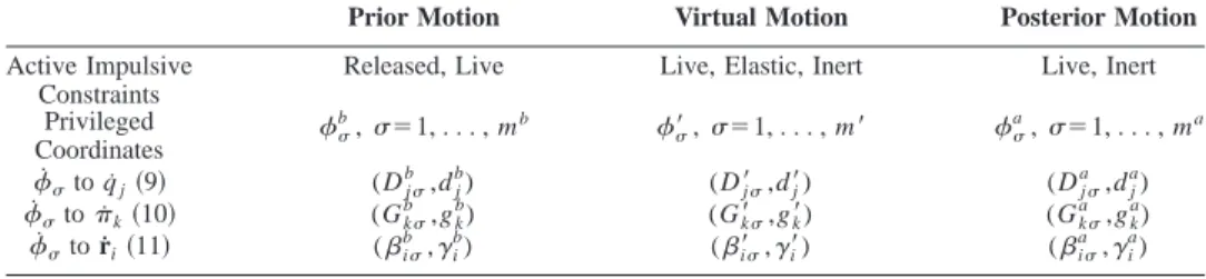
Analogous to the process of selecting the virtual-privileged ve-locities, the set of prior-privileged velocities 兵˙b其, and that of posterior-privileged velocities兵˙a其can be obtained for the prior motion and the posterior motion, respectively. Similar forms of Eqs.共9兲, 共10兲, 共11兲 are found for each phase to describe the mo-tion, with the corresponding notations summarized in Table 1. It is noted that the selection of privileged velocities basically depends on the coefficients of the velocity terms, i.e., Bs j
I , Bs j
R
, and Ck j, and hence the discontinuity of the inhomogeneous terms arising from the live constraints does not affect the selection process.
If all the kinematic constraints are regular, i.e., there is no im-pulsive constraint, the kinematic conditions for the three phases of motion are the same, with the same degree-of-freedom m⬘⫽mb
⫽ma⫽m⫽n⫺L. The same set of privileged velocities may be selected as well to describe the motion for three phases, i.e.,˙⬘ ⫽˙b⫽˙a⫽˙, ⫽1,¯ ,m. The problem is then simplified to the classical problem of impulsive motion, and the method pre-sented in this paper is similar to the one used in关7兴.
An impulsive problem that the prior motion is given and the posterior motion is to be determined is called a prior-value prob-lem共analogous to the initial-value problem for differential equa-tions兲. For such problems, the posterior velocity of each particle Piin S can be expressed in terms of the posterior-privileged ve-locities evaluated at t¯⫹ as vi共⫹兲⫽
兺
⫽1 ma i a共q¯, t¯兲˙ a共⫹兲⫹␥ i a共 t¯⫹兲, i苸I. (12) From the previous equations, once the posterior-privileged veloci-ties are determined, the posterior velocity of each particle inS can be obtained subsequently.To solve the prior-value problem, fundamental principles in me-chanics needs to be invoked. To deal with the systems subject to constraints for finite-force problems, many variational principles have been developed, in which the concept of variations is intro-duced to ‘‘test’’ the limitations from the constraints. These varia-tions are essentially infinitesimal quantities imposed on the system variables. As reviewed in关25兴, there are basically three types of variations. In the principle of virtual work or D’Alembert’s prin-ciple in dynamics, the virtual displacement is an infinitesimal and instantaneous displacement imposed on the configuration of the system. In the principle of least constraint or the Gauss principle, 关36兴, the variation is imposed on the acceleration of each particle while keeping the time, the position, and the velocity unchanged. On the other hand, in Jourdain’s principle,关22,23兴, or the principle of virtual power,关24,26兴, the variation is on the velocity, denoted by ␦1vi, which is instantaneous (␦1t⫽0) and stationary (␦1ri
⫽0).
In the literature, the term of virtual displacement and that of virtual velocity are sometimes used interchangeably. This may be due to the reason that in the original work of Bernoulli关37兴, the principle of virtual work is called the principle of virtual velocity. To tell the difference between the virtual displacement and the variation of velocity defined above, the latter shall be termed the velocity variation in this paper. In modern geometric mechanics, the virtual displacement is viewed as a tangent vector to the con-figuration space, 关38兴, due to its infinitesimal character. Analo-gously, the velocity variation may be treated as a tangent vector to the velocity space, and is thus intrinsically different from the no-tion of virtual displacement.
The velocity variation plays a central role in the fundamental principle for impulsive motion presented in the next section, which requires that they must be compatible with the kinematic conditions of constraints in the virtual motion. From the above discussions, any possible velocity of each particle in virtual mo-tion can be represented in terms of the virtual-privileged
veloci-ties, Eq.共11兲. By taking␦1-variation on共11兲, the velocity varia-tion␦1r˙ican be then expressed in terms of the variations of the virtual-privileged velocities␦1˙⬘ as
␦1r˙i⫽
兺
⫽1 m⬘
i⬘共q,t兲␦1˙⬘, i苸I. (13) Since the virtual-privileged velocities˙⬘are independent, there is no constraint on the corresponding variations ␦1˙⬘. This fact shall be used in the next section to establish the required equations of jumps from the variational equation.
4 Kinetic Equations for Impulsive Motions
The dynamics of impulsive motion may be thought of as the limiting case for a finite-force problem. In addition to the D’Alembert-Lagrange equation and the Gauss-Gibbs equation, Jourdain in 1909, 关22兴, established a variational equation for systems subject to linear kinematic constraints in terms of the infinitesimal variation of velocities. Later, Pars关3兴 extended the equations to accommodate the finite variations of velocities, and obtained the so-called second form of the fundamental equa-tions as
兺
i苸I 共mir¨i⫺Fi共A兲兲•⌬1r˙i⫽0, (14)
where r¨iis the actual acceleration of particle Pi, Fi (A)
denotes the resultant applied force acting on Pi, and⌬1r˙iis an arbitrary finite or infinitesimal variation of possible velocity compatible with the constraints.
To extend the previous variational equation to deal with the constrained impulsive problem, due to the appearance of the im-pulsive constraints, the set of conditions from the constraints with which the velocity variations must be compatible should be iden-tified. It may be envisioned that during the impulsive motion, the system undergoes the stage of virtual motion, during which the system satisfies the kinematic conditions from the regular con-straints and the impulsive concon-straints including the types of inert, elastic, and live. As a result, the velocity variations for virtual motion must be compatible with the conditions induced from these kinematic conditions. Substituting Eq. 共13兲 into Eq. 共14兲, and noting the independency of兵␦1˙⬘其⫽1,¯ ,m⬘, we obtain
兺
i苸I 共mir¨i⫺Fi 共A兲兲•i
⬘⫽0, ⫽1,¯ ,m⬘,
where the acceleration of each particle Pimay be very large dur-ing the impulsive motion, and leads to the jump of the correspond-ing velocity.
To obtain the relation between the prior motion and the poste-rior motion for the system S, the previous equations are further expressed as
Table 1 Summary of the transformations
Prior Motion Virtual Motion Posterior Motion Active Impulsive
Constraints
Released, Live Live, Elastic, Inert Live, Inert Privileged Coordinates b ,⫽1, . . . , mb ⬘,⫽1, . . . , m⬘ a,⫽1, . . . , ma ˙to q˙j共9兲 (Djb ,dj b ) (D⬘j,dj⬘) (Dja,dj a ) ˙to˙k共10兲 (G k b ,gk b ) (Gk⬘,gk⬘) (Gk a ,gk a ) ˙to r˙i共11兲 (ib,␥i b) ( i ⬘ ,␥i⬘) (ia,␥i a)
d dt
冉
兺
i苸I mir˙i•i⬘冊
⫺兺
i苸I mir˙i•冉
兺
j⫽1 n i⬘ qj q ˙j⫹ i⬘ t冊
⫺兺
i苸I F共A兲i •i⬘⫽0, ⫽1,¯ ,m⬘. (15)Since i⬘ is continuous and the velocities, r˙i, i苸I, and q˙j, j
⫽1,¯ ,n are finite, the second term in the previous equation is finite for each ⫽1,¯ ,m⬘. Let theth virtual-privileged mo-mentum ofS and theth virtual-privileged applied force acting on S be defined as L,
兺
i苸I mir˙i•i⬘共q,t兲, (16) F共A兲,兺
i苸I Fi共A兲•i⬘共q,t兲, (17) respectively. Integrating Eq.共15兲 from t¯⫺ to t¯⫹, and letting →0, the second term vanishes, and the privilegedimpulse-momentum equations can be established:
L共⫹兲⫺L共⫺兲⫽P共A兲, ⫽1,¯ ,m⬘, (18) where L共⫺兲,
兺
i苸I mivi共⫺兲•i⬘共q¯, t¯兲, (19) L共⫹兲,兺
i苸I mivi 共⫹兲• i ⬘共q¯, t¯兲, (20)denote the th prior and posterior virtual-privileged momenta, respectively, and P共A兲,
冕
t¯⫺ t¯⫹ F共A兲dt⫽冕
t¯⫺ t¯⫹兺
i苸I F共A兲i •i⬘共q,t兲dt (21) is theth virtual-privileged applied impulse.Again, by the continuity of i⬘ and the negligible change of configuration and interval of time during the impulsive motion, the virtual-privileged applied impulses can be further expressed as
P共A兲⫽
兺
i苸I冉
冕
t¯⫺ t¯⫹ Fi共A兲dt冊
•i⬘共q¯, t¯兲⫽兺
i苸I Pi共A兲•¯i⬘, ⫽1,¯ ,m⬘, (22) where Pi (A),兰 t¯⫺ t¯⫹ Fi (A)dt is the applied impulse acting on particle Pi, i苸I. Substituting the previous equation into 共18兲, the privi-leged impulse-momentum equations are rewritten as
兺
i苸I 共mivi 共⫹兲⫺miv i 共⫺兲⫺P i 共A兲兲• i ⬘共q¯, t¯兲⫽0, ⫽1,¯ ,m⬘. (23) From Eq.共22兲, given applied impulses acting on S, the virtual-privileged applied impulses can be determined, and the jumps of the m⬘virtual-privileged momenta defined as⌬L,L共⫹兲⫺L共⫺兲 , ⫽1,¯ ,m⬘, (24) are then obtained from Eq.共23兲.
The above derivation of the privileged impulse-momentum equations is based on the framework for finite-force problems. To gain more direct insight on the impulsive motion subject to con-straints, and to avoid the technicalities in the transition from finite-force problems to impulsive problems, one may follow the principle of velocity variations for constrained impulsive motion as stated below:
Consider a system of particles Pi, i苸I, connected with one another in any way. The system may be subjected to applied
im-pulses Pi (A)
on particle Pi. These applied impulses would impart to the free particles certain determinate jumps on their velocities. However, due to the constraints, regular or impulsive, the actual jumps are different from those on the free motions. Conceive that the applied impulse Pi
(A)
be resolved into the effective impulse Pi(E)⫽mivi
(⫹)⫺m ivi
(⫺), and another component termed the net applied impulse. Owing to the constraints, only the effective im-pulses generate the actual jumps. The net applied imim-pulses are incapable to change the jumps during the impulsive motion, and the sum total of the product of the net applied impulses and the velocity variations compatible with the constraints during the vir-tual motion must vanish.
This principle is an analog of the principle of virtual power for finite-force motion stated in关26兴, and the statements are similar to the exposition of D’Alembert’s principle by Mach关37兴. It is noted that Appell in关1兴 enunciated a fundamental principle for impul-sive motion analogous to D’Alembert’s principle, and, based on which, established the general variational equation in terms of virtual displacements. However, as discussed before, a virtual dis-placement refers to a variation of the position of the particle, which is in fact not allowed during the impulsive motion. While the variational equation corresponds to the previous principle has similar characteristics as that derived by Appell, the notion of velocity variation while keeping position fixed is more acceptable for the impulsive motion.
Based on this fundamental principle, the corresponding varia-tional equation for impulsive motion can be immediately ex-pressed as
兺
i苸I 共mivi 共⫹兲⫺mivi共⫺兲⫺Pi共A兲兲•␦1r˙i⫽0, (25) for all␦1r˙i compatible with the constraints specified during the virtual motion at (q¯, t¯). Substituting共13兲 into the previous varia-tional equation and noting the independency of the variations of the virtual-privileged velocities, the privileged impulse-momentum Eqs. 共23兲 immediately follow. This process may be viewed as the projection from the space of␦1r˙i to that of␦1˙⬘ through Eq.共13兲, and is essentially the basic idea for the so-called projection method,关29,30兴. Similar techniques were also used in 关12,31兴 to derive jump conditions from a variational equation similar to共25兲 in virtual displacement without applied impulse. There the projection is from the tangent bundle to the distribution that annihilates the constraint submanifold. Since the velocity variations should reside in the second tangent bundle, or the jet space of order 2, the projection throughi⬘should be regarded as different from those in the tangent bundle.
Moreover, it is noted that the projection in Eq. 共13兲 does not depend on the velocity. This is due to the fact that only linear kinematic constraints are treated in this paper. If the system is subject to nonlinear ones in the form of (x1,¯ ,x3N,x˙1,¯ ,x˙3N,t)⫽0, the projection or the transforma-tion may depend on the velocities. For impulsive problems, the discontinuity of the velocity then renders the transformation inde-terminant. In关12兴, the impulsive constraints are associated with Chetaev bundle,关39兴, of reaction forces from the constraints, lin-ear or nonlinlin-ear. However, if the kinematic constraint is nonlinlin-ear, it is not clear how to compute the corresponding impulse of these Chetaev forces, which depends on the velocity in general. As a result, more understandings on the mechanism for the impulsive motion subject to nonlinear kinematic constraints are desired. 5 Prior-Value Problems
We are now ready to apply the privileged impulse-momentum equations to study constrained impulsive problems. In the absence of applied impulses, from共18兲, we immediately have the follow-ing conservation law for constrained impulsive motion: the virtual-privileged momenta of the system are conserved if there is no applied impulse.
For the prior-value problem, the prior virtual-privileged mo-mentum can be computed from the state of the prior motion through Eq.共19兲. The posterior virtual-privileged momentum is then determined from the privileged impulse-momentum Eq.共23兲. To find the posterior motion, the relation between the m⬘posterior virtual-privileged momenta and the ma posterior-privileged ve-locities is constructed by substituting共12兲 into 共20兲,
L共⫹兲⬘ ⫽
兺
⫽1 ma冉
兺
i苸I mi¯i⬘⬘•¯ai冊
˙a共 t¯⫹兲⫹兺
i苸I mi¯i⬘⬘•␥i a共 t¯⫹兲 ⫽兺
⫽1 ma M⬘˙a共 t¯⫹兲⫹L共⫹兲⬘0, ⬘⫽1,¯ ,m⬘, (26) where M⬘,兺
i苸I mi¯i⬘⬘•¯i a , L共⫹兲⬘0,兺
i苸I mi¯i⬘⬘•␥i a共 t¯⫹兲.Here, and in what follows, the overbar of a continuous quantity denotes its value at (q¯, t¯), e.g.,¯ia⫽ia(q¯, t¯).
The previous set of m⬘ Eqs.共26兲 is to be solved for the ma (⫽n⫺L⫺lL⫺lI) unknowns,˙a( t¯⫹), ⫽1,¯ ,ma. The differ-ence between the number of equations and that of unknowns is lE, which is the number of elastic constraints. As a result, it is not possible to determine the posterior motion without additional lE conditions if elastic constraints exist. Such conditions may be ob-tained by invoking the law of impact, cf.关2,19兴, or 关27,40兴 for more recent developments. For example, to determine the poste-rior motion of a ball being dropped to the floor, the coefficient of restitution is needed to find the extend of rebound. The elastic constraint is r˙"n⫽0, where n is the normal vector corresponding the floor, and the posterior velocity is related to the prior velocity as
v共⫹兲•n⫽⫺v共⫺兲•n.
From the previous example, it may be conceived that for the elastic constraints, 兺jn⫽1Bs jEq˙j⫹bsE⫽0, s⫽1,¯ ,lE, there are lE generalized coefficients of restitution s to bear the relationship between the ‘‘approaching’’ constraint functions and the ‘‘leav-ing’’ constraint functions as
兺
j⫽1 n B ¯ s j Eq˙ j 共⫹兲⫹b¯ s E⫽⫺ s冉
兺
j⫽1 n B ¯ s j Eq˙ j 共⫺兲⫹b¯ s E冊
, s⫽1,¯ ,l E, where the coefficients and the inhomogeneous terms are assumed to be continuous. From the formula of the posterior generalized velocities, with coefficients listed in Table 1, the previous equa-tions are further expressed as兺
⫽1 ma冉
兺
j⫽1 n B ¯ s j ED¯ j a冊
˙ a共 t¯⫹兲 ⫽⫺兺
j⫽1 n B ¯ s j E共d j a共 t¯⫹兲⫹ sq˙共⫺兲j 兲⫺共1⫹s兲b¯sE, s⫽1,¯ ,lE. (27) Equations 共26兲, 共27兲 can be then combined to obtain the ma posterior-privileged velocities, as illustrated by the following simple example.Example 1. Consider a particle of mass m being tossed to the floor (z⫽0) with prior velocity vx
(⫺) ex⫹vz
(⫺)
ez. Assume that the sur-face of the floor is ideally smooth, and the coefficient of restitu-tion of the contact is. It is desired to determine the posterior velocity of the particle.
The impulsive constraint provided by the floor is z˙⫽0, which is an elastic constraint. Hence, the virtual motion can be expressed as r˙⫽x˙ex, where x˙ can be selected as the privileged velocity for
the virtual motion, and the coefficient corresponding to x˙ is¯1⬘
⫽ex. The prior and posterior virtual-privileged momentum can be found to be L1 (⫺)⫽(mv x (⫺)e x⫹mvz (⫺)e z)•ex⫽mvx (⫺), L 1 (⫹) ⫽(mvx (⫹)e x⫹mvz (⫹)e z)•ex⫽mvx
(⫹), respectively. The conserva-tion of the virtual-privileged momentum leads to vx(⫺)⫽vx(⫹). However, this equation is not sufficient to determine all the pos-terior velocities. The additional condition from the law of impact, i.e., vz(⫹)⫽⫺vz(⫺), is needed to obtain the posterior velocity vx(⫺)
ex⫺vz (⫺)
ez. 䊐
In contrast to the previous case for an impulsive motion without elastic constraint, we have the same number of unknowns and equations in共26兲, and the coefficients¯i
a⫽¯ i
⬘ if the same set of virtual-privileged velocities and posterior-privileged velocities is chosen. Accordingly, the matrixMformed by the components
M⬘⫽
兺
i苸Imi¯i⬘⬘•¯⬘i, ,⬘⫽1,¯ ,m⬘, (28) is positive definite and shall be termed the privileged mass matrix. Under this framework, the posterior-privileged velocities can be obtained from the following equations:
˙a共⫹兲⫽
兺
⬘⫽1 m⬘ 共M⫺1兲⬘共L ⬘ 共⫹兲⫺L ⬘0 共⫹兲兲, ⫽1,¯ ,m⬘, (29) from which the posterior velocities can be determined from共12兲. For the treatment of released constraints, the above deduction of determinacy is apparently different from that claimed in关8兴, which regards the third type of impulsive problem in关1兴 as inde-terminant. To illustrate the difference, we consider again the prob-lem of releasing a ball from hand grasping. As described in Sec-tion 2, the constraint of grasping is treated as a released constraint, which is effective before but ineffective during and after the im-pulsive motion. Since there is no kinematic constraint imposed in the virtual motion, the virtual-privileged velocities of the ball can be selected to be the three components of the linear velocity of the ball, and the corresponding virtual-privileged momenta are noth-ing but the three components of the linear momentum M v. If hand does not provide additional applied impulse, from the conserva-tion law of virtual-privileged momenta, we have M v(⫺)⫽Mv(⫹) ⫽0 if the ball is released from rest. The posterior motion is then determined, and the motion of the ball bears no sudden change during the impulsive motion, only experiences sudden increase of the degree-of-freedom. From this simple example, it is seen that the notion of released constraint introduced in this paper is more appropriate to be adopted to treat the released constraints from grasping.Now we consider the special case that there is neither inert constraints nor released constraints existing, while some live con-straints appear. For such impulsive motion, as discussed in the previous section, the same set of privileged velocities may be chosen for the prior motion and the posterior motion,˙b⫽˙a, where⫽1,¯ ,ma(⫽mb⫽n⫺L⫺lL), and we have
v共⫺兲i ⫽
兺
⫽1 ma ¯i a˙ a共⫺兲⫹␥ i a共 t¯⫺兲, (30) vi共⫹兲⫽兺
⫽1 ma ¯i a˙ a共⫹兲⫹␥ i a共 t¯⫹兲, i苸I. (31)The privileged impulse-momentum Eqs.共23兲 then implies that
兺
⫽1 ma
where⌬˙⫽˙a(⫹)⫺˙a(⫺), and⌬L⬘0⫽L⬘0 (⫹)⫺L
⬘0
(⫺). Moreover, if there is no elastic constraint, we have m⬘⫽ma⫽mb⫽n⫺L ⫺lL, and the jumps on the privileged velocities can be found from ⌬˙⫽
兺
⬘⫽1 m⬘ 共M⫺1兲⬘共⫺⌬L⬘0⫹P共A兲⬘兲, ⫽1,¯ ,m⬘. (33) With the prior quantities˙a(⫺) being determined from the prior motion, the posterior quantities˙a(⫹)are then computed from the previous equation, which, in turn, yield the posterior velocities of the system through Eq.共12兲.After systematically discussing the impulsive motion associated with various impulsive constraints, the special case that the sys-tem is subject to applied impulses with only regular constraints being active is considered next. Since the kinematic conditions are the same for the prior, the virtual, and the posterior motion, the same set of privileged velocities can be chosen, denote by ˙1,¯ ,˙m, with the same degree-of-freedom m⫽n⫺L. The cor-responding coefficients for the velocity of each particle in three phases are thus the same, denoted by兵i,␥i其i苸I,⫽1,¯ ,m. Simi-lar to the special treatment on the live constraints, the privileged impulse-momentum equations become, cf. Eq.共32兲,
兺
⫽1 m M⬘⌬˙⫽P ⬘ 共A兲, ⬘⫽1,¯ ,m, (34)since⌬L⬘0⫽0 due to the nonexistence of live constraints. By computing the privileged applied impulses from the formula
P共A兲⬘⫽
兺
i苸I Pi共A兲•¯
i⬘, ⬘⫽1,¯ ,m, (35)
and the privileged mass matrix from M⬘⫽
兺
i苸I
mi¯i•¯i⬘, ,⬘⫽1,¯ ,m, (36) the jumps on the privileged velocities can be determined from Eq. 共34兲, and the posterior velocities of the system can be found sub-sequently from Eq.共12兲.
6 Impulsive Motion for a System Containing Rigid Bodies
A finite degree-of-freedom mechanical systemS may be com-posed of many particles and rigid bodies. The physical quantities such as the virtual-privileged momenta and the virtual-privileged applied impulses can be defined for each subsystem. Due to the superposition property of the Eq. 共23兲 with respect to the sub-systems, a physical quantity for the systemS can be obtained by taking the summation of the corresponding ones of all subsystems. The motion of a rigid body B in S may be described by the translational motion of some reference point Q inB and a rota-tion about Q, represented by the rotarota-tion dyadic⌽. The rotation dyadic⌽ changes the attitude of the rigid body from a reference 共initial兲 configuration to the current configuration, and satisfies the property
⌽•⌽c⫽1, det ⌽⫽1,
where⌽cdenotes the conjugate of⌽, and 1 is the identity dyadic. It can be shown from the previous defining property that
⌽˙⫽⫻⌽, (37)
in dyadic notation,关41兴, where is the angular velocity of the rigid body. The position vector of any point P苸B can be then expressed as
rP共t兲⫽rQ共t兲⫹⌽共t兲•RPQ,
where RPQdenotes the vector from P to Q at the reference con-figuration. Taking the time-derivative of the previous equation, we obtain
r˙P⫽r˙Q⫹⫻⌽•RPQ⫽r˙Q⫹⫻共rP⫺rQ兲. (38) Now let (q1,¯ ,qn) be a set of generalized coordinates ofS. In general, the rotation dyadic ⌽ may be written in terms of the generalized coordinates as ⌽⫽⌽(q1,¯ ,qn,t), and its time-derivative is ⌽˙⫽
兺
i⫽1 n ⌽ qi q ˙i⫹ ⌽ t .From the previous equation and Eq.共37兲, the expression of the angular velocity in terms of the generalized velocities can be derived from the following identity:
1⫻⫽⌽˙•⌽C⫽
兺
i⫽1 n冉
⌽ qi•⌽ C冊
q˙ i⫹ ⌽ t •⌽C, as ⫽兺
i⫽1 n ˆi共q,t兲q˙i⫹ˆ0共q,t兲. (39) In general, the right-hand side in the previous equation is not integrable, and the components of with respect to certain frame can be treated as quasi-velocities of the system, cf. Eq.共7兲.Consider the virtual motion ofS during a constrained impulsive motion. With the appropriate selection of virtual-privileged ve-locities, ˙⬘, the velocities of the reference point Q and each particle P inB can be expressed in the form of 共11兲 with coeffi-cients (␥Q⬘,Q0⬘ ), (⬘P,␥P⬘), ⫽1,¯ ,m⬘, respectively, and the angular velocity ofB is further written as
⫽
兺
⫽1 m⬘
⬘˙⬘⫹0⬘. (40)
Substituting these expressions into Eq.共38兲, it follows that
兺
⫽1 m⬘ 共P⬘⫺Q⬘兲˙⬘⫹共␥P⬘⫺␥Q⬘兲 ⫽兺
⫽1 m⬘ ⬘⫻共rP⫺rQ兲˙⬘⫹0⬘⫻共rP⫺rQ兲, which leads to P⬘⫺Q⬘⫽⬘⫻共rP⫺rQ兲, ␥P⬘⫺␥Q⬘⫽0⬘⫻共rP⫺rQ兲, (41) for⫽1,¯ ,m⬘, by the independency and the arbitrariness of the virtual-privileged velocities.These relations, which based on the kinematic properties of a rigid body, are now applied to derive the prior and posterior virtual-privileged momenta, and virtual-privileged applied im-pulses for the rigid bodyB as follows. From Eqs. 共19兲, 共20兲, with the index set I being over P苸B, we have
LB共⫾兲,
冕
B v共⫾兲P •¯P⬘dm共P兲 ⫽冕
B vP共⫾兲•关¯Q⬘⫹¯⬘⫻共rP⫺rQ兲兴dm共P兲 ⫽LB共⫾兲•¯ Q ⬘ ⫹HQB共⫾兲•¯⬘, ⫽1,¯ ,m⬘, (42) whereLB共⫾兲⫽
冕
BvP共⫾兲dm共P兲 (43) are the prior and posterior linear momenta ofB, respectively, and
HQB共⫾兲⫽
冕
B共rP⫺rQ兲⫻vP
共⫾兲dm共P兲 (44)
are the prior and posterior angular momenta ofB about the refer-ence point Q, respectively. Let C denote the center of mass of the rigid body B, and M, IQ be the total mass and the moment of inertia dyadic of the rigid body about Q, respectively. The linear momenta and the angular momenta defined in 共43兲, 共44兲 can be further expressed as
LB共⫾兲⫽MvC共⫾兲, (45) HQB共⫾兲⫽IQ•共⫾兲⫹共rC⫺rQ兲⫻共MvQ共⫾兲兲, (46) respectively.
On the other hand, the virtual-privileged applied impulses cor-responding toB can be found to be, using Eq. 共41兲,
PB共A兲,
兺
P苸B P共A兲P •¯P⬘⫽兺
P苸B PP共A兲•关¯Q⬘⫹¯⬘⫻共rP⫺rQ兲兴 ⫽PB共A兲•¯ Q ⬘ ⫹JQ B共A兲•¯ ⬘, ⫽1,¯ ,m⬘, (47) where PB(A), J QB(A)are the resultant applied linear impulse, and the applied angular impulse acting onB about Q, defined as
PB共A兲⫽
兺
P苸BPP 共A兲, (48) JQB共A兲⫽兺
P苸B共rP⫺rQ兲⫻PP 共A兲, (49) respectively.After obtaining the formula for a single rigid body, the virtual-privileged momenta and applied impulses for the system consist-ing many bodies can be constructed. Let the system be composed of NBrigid bodies, which may be expressed as
S⫽ 艛 i⫽1
NB Bi.
For each body i,i⫽1, . . . NB, we may choose a reference point Qi, and denote the attitude dyadic by⌽i. With the selection of privileged velocities ofS in the virtual motion, the coefficients (⬘)Bi and 
Qi
⬘ for each body can be determined. The virtual-privileged momenta and the applied impulses of the system are then found from the following summation:
L共⫾兲⫽
兺
i⫽1 NB LBi共⫾兲, P共A兲⫽兺
i⫽1 NB PBi共A兲, (50)respectively. With these formulas, the privileged impulse-momentum equations developed in Section 4 can be invoked to solve the constrained impulsive problems associated with inter-connected rigid bodies. An example is given in the next section to illustrate the process.
7 The Impulsive Motion of a Sleigh With a Knifeblade The proposed methodology discussed in the previous sections is now applied to study the impulsive motion of a sleigh with a knifeblade attached. Three possibilities of impulsive motions due to applied impulse, inert constraint, and live constraint, re-spectively, are discussed. Two alternative methods, namely, New-ton’s method and Lagrange’s method, are used to solve the same problem for the case of inert constraint to describe the essential differences.
Consider a sleigh B with a knifeblade along its principle axis, as depicted in Fig. 2. Let its mass and moment of inertia about its center of mass C be denoted by M and IC, respectively. When the sleigh moves on a horizontal ice surface S, it is assumed that the knifeblade makes contact with the surface at point A, and it is possible for the sleigh to move freely in the direction along the blade, and rotate freely about A. However, the motion of the sleigh in the direction perpendicular to the blade is prohibited. Let兵i, j其 be a fixed coordinate system, and兵ex,ey其be a coordinate system moving withB, where exis parallel to the direction of the blade, which makes an angle with respect to the axis i. Due to the physical condition of constraints, the velocity of A satisfies
vA•ey⫽0, (51)
and may be expressed as
vA⫽uex, (52)
where u is termed the longitudinal velocity ofB. The sleigh may rotate about the vertical axis ez(⫽ex⫻ey) with angular velocity
˙ez. The velocity of C may be then expressed as
vC⫽uex⫹l˙ey, (53)
where l denotes the distance between C and A. For this prob-lem, we may choose the coordinates of C, i.e., (xC,yC), and the angle as the generalized coordinates. The constraints 共51兲 then becomes
⫺sinx˙C⫹cosy˙C⫺l˙⫽0, (54)
which is nonholonomic. The longitudinal velocity u can be ex-pressed as
u⫽cosx˙C⫹siny˙C, Fig. 2 The impulsive motion of a sleigh with a knifeblade
in which the right-hand side is not integrable, and thus should be treated as a quasi-velocity.
We are now ready to consider three cases of impulsive motions for this system, which occur at the instant t¯ and at the configura-tion of⫽0.
Case (i). As shown in Fig. 2共i兲, the sleigh is suddenly exerted by an impulse P acting at the point D at the instant t¯. The longitu-dinal velocity ofB and the angular velocity of B about the vertical axis at the instant t¯⫺ are u(⫺)and˙(⫺), respectively. It is desired to determine these two quantities at the instant t¯⫹.
For this case, the impulsive motion is due to the imposition of the applied impulse P, while the rigid body B is subject to the regular nonholonomic constraint, Eq.共54兲. One may choose the longitudinal velocity u and the angular velocity˙ as the privileged velocities to represent the possible motion ofB. In fact, the ve-locity of A and C can be written in terms of the privileged veloci-ties as in Eqs.共52兲 and 共53兲, respectively. Since the prior and the posterior motions satisfy the same nonholonomic constraint, the prior and posterior velocities of A and C, vA
(⫺) , vC (⫺) , vA (⫹) and vC (⫹)
, can be also expressed in terms of the prior and posterior-privileged velocities, u(⫺), ˙(⫺), u(⫹), and˙(⫹), with the same form, respectively.
Let C be selected as the reference point forB. The coefficients of the velocity of C and the angular velocity ofB corresponding to the privileged velocities can be obtained as
¯C1⫽ex, ¯C2⫽ley,
(55) ¯1⫽0, ¯2⫽ez,
respectively. The linear momenta, and the angular momenta about C given in共43兲, 共44兲, are then
LB共⫾兲⫽Mu共⫾兲ex⫹Ml˙共⫾兲ey, HCB共⫾兲⫽IC˙共⫾兲ez,
respectively. On the other hand, the applied linear impulse and the applied angular impulse are, respectively,
PB共A兲⫽Pey, JCB共A兲⫽Pae
z.
Substituting these terms into the formula of the privileged mo-menta and privileged applied impulses, the privileged impulse-momentum Eq.共18兲 can be applied to derive, in matrix form,
关M兴
冉冋
u 共⫹兲 ˙共⫹兲册
⫺冋
u共⫺兲 ˙共⫺兲册冊
⫽冋
0 P共a⫹l兲册
, where the privileged mass matrix关M兴 is given by关M兴⫽
冋
M 00 共Ml2⫹IC兲
册
. (56)
Hence, the posterior longitudinal velocity and angular velocity of the sleighB can be determined as
冋
u共⫹兲 ˙共⫹兲册
⫽关M兴⫺1冋
0 P共a⫹l兲册
⫹冋
u共⫺兲 ˙共⫺兲册
⫽冋
u共⫺兲 a⫹l M l2⫹IC P⫹˙共⫺兲册
. 䊐Case (ii). Consider the landing of the sleigh on the ice surface at the instant t¯, with prior velocity of the center of mass beingvC
(⫺) in the direction of angle(⫺) with respect to the axis i, and the prior angular velocity about ezbeing˙(⫺), cf. Fig. 2共ii兲. The ve-locity of the landing point A may have lateral component before t¯, but it immediately satisfies the constraint共51兲 after contact. This impulsive constraint is thus characterized as an inert constraint. The virtual motion and the posterior motion have the same char-acteristics as the motion in Case 共i兲. Similar to the discussion
there, the set of velocities (u,˙) may be chosen as the virtual-privileged velocities, ˙1⬘⫽u, ˙2⬘⫽˙. However, they are not the privileged velocities for the prior motion. Again, the point C is chosen as the reference point forB, and the coefficients for the velocity of C and the angular velocity ofB corresponding to the virtual-privileged velocities are the same as in 共55兲, with ¯, ¯ being replaced by ¯⬘, ¯⬘ respectively. The required quantities can be found to be
LB共⫺兲⫽Mv
C
共⫺兲cos共共⫺兲⫺
0兲ex⫹MvC共⫺兲sin共共⫺兲⫺0兲ey, LB共⫹兲⫽Mu共⫹兲ex⫹Ml˙共⫹兲ey,
HCB共⫾兲⫽I
C˙共⫾兲ez.
The prior and the posterior virtual-privileged momenta corre-sponding respectively to1⬘, 2⬘are then
L1共⫺兲⫽MvC共⫺兲cos共共⫺兲⫺0兲, L1共⫹兲⫽Mu共⫹兲,
L2共⫺兲⫽MlvC共⫺兲sin共共⫺兲⫺0兲⫹IC˙共⫺兲, L2共⫹兲⫽共Ml2⫹I
C兲˙共⫹兲.
Since there is no applied impulse, the conservation of virtual-privileged momenta can be then invoked to yield the posterior velocities as u共⫹兲⫽vC共⫺兲cos共共⫺兲⫺0兲, ˙共⫹兲⫽ 1 M l2⫹I C共MlvC 共⫺兲sin共共⫺兲⫺ 0兲⫹IC˙共⫺兲兲. (57) 䊐
Case (iii). If the ice surface exhibits a sudden motion at t¯ caused by external agents, such as an earthquake, the sleigh moving on it then experiences an impulsive constraint. Let the velocity of the surface be denoted by vS. Instead of共51兲, the constraint becomes now
共vA⫺vS兲•ey⫽0, (58)
or
vA•ey⫺vS•ey⫽0, (59) in which the inhomogeneous term makes it become a live impul-sive constraint. In particular, let the surface suddenly move with velocity vS(⫹) in the direction of angleS(⫹) with respect to the axis i. The velocity of A and C during the impulsive motion can be then expressed as
vA⫽uex⫹vS共cosSi⫹sinSj兲, vC⫽uex⫹l˙ey⫹vS共cosSi⫹sinSj兲,
respectively, in which u is now the longitudinal velocity of the sleigh relative to the surface, andvS, Sare the magnitude and the direction of vS, respectively. From the constraint, we have
vS共 t¯⫺兲⫽0, vS共 t¯⫹兲⫽vS共⫹兲,
S共 t¯⫺兲⫽0, S共 t¯⫹兲⫽S共⫹兲.
For this case, the prior motion, the virtual motion, and the poste-rior motion have the same degree-of-freedom, and the same set of privileged velocities ˙1⬘⫽u, ˙2⬘⫽˙ may be chosen. Again, Eq.
共55兲, after replacing¯, ¯ by¯⬘,¯⬘, is applicable, and the quan-tities of momenta for the body are found as
LB共⫺兲⫽M共u共⫺兲ex⫹l˙共⫺兲ey兲, LB共⫹兲⫽M关u共⫹兲ex⫹l˙共⫹兲ey⫹v S 共⫹兲共cos S 共⫹兲i⫹sin S 共⫹兲j兲兴,