國立高雄大學資訊工程學系(研究所)
碩士論文
整合多資料來源可篩除項目集
Integrating Erasable itemsets from Multiple
Data Sources
研究生:石宗達 撰
指導教授:洪宗貝 博士
致謝
為期兩年的研究所生涯在這篇論文完成之時畫下了句點。在這兩年中,我受 到系上大家的幫忙與照顧,有太多需要感謝的人事物。回憶起三年前我工作上的 主管問起我中程的職涯規劃時,我便興起了回學校再進修的念頭,而主管也應允 了我的想法與計畫,因而開始了這兩年的學生與研究時光。 首先,我當然要感謝的是我的指導教授,洪宗貝博士。在我一開始選擇高雄 大學作為入學目標時,我便也決定要請洪老師當我的碩士論文指導教授。老師在 論文及研究的方法上總是能夠提供許多建議,而且有很多細節上的處理方式都是 一般人不會考慮如此周到的,讓我感到格外受用。除此之外,老師也會教導我們 處理研究外的各種問題,像是人際互動關係、對事情的看法和價值觀的分享等等, 讓我學到除了做好學生的本分之外,在思想上也有許多啟發。 同時,也要感謝我的碩士學位考試口試委員:王學亮校長、林浚瑋教授及蘇 家輝教授。謝謝你們撥冗來參加,並對於我的碩士論文的內容給予寶貴的建議, 使我的論文更加完善且嚴謹。 我也要感謝人工智慧實驗室的大家,這兩年的研究生活因為有你們的陪伴而 感到充實愉快。感謝實驗室的大家,菊添學長、明泰學長、偉銘學長、正男學長、 昆毅、元慶、敏賢、雨棠、仁豪、世祺、冀正,和你們相處的這些日子裡,不論 是研究或娛樂各方面都受到你們的幫忙與照顧。 最後也是最重要的,我必須深深地感謝我的老婆跟女兒,每當我心情煩躁 或工作繁忙之時,總是能適時給予鞭策與鼓勵。你們在這兩年來對我的付出與 關懷,使得我能致力於研究上,因為有你們的支持,我才能夠順利地完成學 業,謝謝你們。 石宗達 2016.07.30 謹誌於 楠梓 國立高雄大學整合多資料來源可篩除項目集
指導教授:洪宗貝 博士 國立高雄大學資訊工程所 學生:石宗達 國立高雄大學資訊工程所 摘要 可篩除項目集之探勘是一種適用於工廠生產規劃的新奇且有趣的問題。它的 目的是要探勘出某些可篩除的項目集(元件),其由這些項目所製造的產品若獲利 小於給定的門檻值,則這些項目即可從製造工廠中刪除。可篩除項目集可用於當 工廠需要更新產品項目或產品項目需要減少以因應生產瘦身的需求且仍能保持 營運且獲利時。由於一個公司可能會有好幾個工廠,而每一個工廠也可能會在一 固定時間(月或季)探勘獲得其各自工廠之可篩除項目集,以作為個別工廠營運分 析之用。而總公司的經理層則可能需要知道所有的工廠整體考量時的可篩除項目 集,以當作未來整個公司營運決策準則。在本論文中,我們將探討從多個資料來 源之可篩除項目集之整合問題。基於在每個各別運作的工廠的可篩除項目集為已 知資訊,我們試圖去減少不必要的資料來源重新掃描以增進在合併可篩除項目集 的效能。我們將先從兩個工廠可篩除項目集的合併開始,提出了一個高效率的演 算方法。項目集分為可篩除和不可篩除,因此在兩個工廠的案例中我們可將所有 的項目集分成四種不同的狀況討論。根據個別的情況,有些可以無需重掃資料庫 而將項目集直接合併以獲得可篩除項目集,而有些則需重新掃描部分的資料庫即 可獲得合併後的結果,如此可減少探勘時間並增進效能。此外,我們可以進一步 擴充兩個工廠可篩除項目集的整合方法去處理兩個以上的可篩除項目集合併需求。最後我們安排了四個不同狀況的實驗,而由實驗結果證明我們所提的演算法 對於整合多個可篩除項目集時可比傳統原有的批次處理探勘方式有更快的執行 速度。
Integrating Erasable itemsets from Multiple Data
Sources
Advisor: Dr. Tzung-Pei Hong
Institute of Computer Science and Information Engineering National University of Kaohsiung
Student: Tsung_Ta Shih
Institute of Computer Science and Information Engineering National University of Kaohsiung
ABSTRACT
Erasable-itemset mining is a new and interesting problem suitable for factory production planning. It is to find the itemsets (components) that can be eliminated if the products generated from them gain profit under a given threshold. Erasable itemsets can be used when a factory needs to renew products or production needs downsizing and can still keep operation and gain profit. A company may have several factories, each of which may derive its own erasable itemsets at a time period. A manager of the company needs to know the overall erasable itemsets integrated from all the factories. In this thesis, we thus consider the erasable-itemset integration to merge the erasable itemsets from multi-sources. It is based on the known erasable itemsets in each factory as a reference information to reduce the rescan of the individidual data sources. We start from two-factory erasable-itemset merging and propose an efficient
integration approach. Itemsets are classified into erasable and non-erasable, and thus four cases can be derived for an itemset in two factories. We can thus get the merged erasable itemset directly or rescan partial data sources to reduce mining time according to the cases. Besides, the proposed two-factory integration approach can be further extended to process more than two sets of erasable itemsets. Four experiments are made and their results show that the proposed algorithm executes faster than the batch approach in the multiple data-source environment for erasable itemsets.
Keywords: data mining, erasable itemset, two-factory integration approach, multiple data sources.
Content
致謝 ... ii 摘要 ... iv ABSTRACT ... vi Content ... viii List of Figures ... xList of Tables ... xxi
CHAPTER 1 Introduction ... 1
1.1 Background and Motivation ... 1
CHAPTER 2 Review of Related Work ... 4
2.1 Erasable-Itemset Mining ... 4
2.2 The Erasable-Itemset Mining Algorithm ... 5
2.3 An Example for Erasable-Itemset Mining ... 7
CHAPTER 3 A Multiple Sources Data mining Algorithm for Mining Erasable Itemsets ... 13
3.1 Main Idea ... 13
3.2 The Terms ... 15
3.3 The Proposed Two-factory Erasable-itemset Merging Algorithm (TEIMA) ... 19
3.4 An Example of the Proposed Algorithm (TEIMA) ... 23
3.5 The Proposed Multiple-factory Erasable-itemset Merging Algorithm (MEIMA)……….37
3.6 An Example of the Proposed Algorithm (MEIMA)……….40
CHAPTER 4 Experiments and Analysis ... 51
4.1 Experimental Environments ... 51
4.2 Experimental Settings ... 51
4.3 Experimental Results ... 52
4.3.1 Experimental Results on two factories merged with same product items number……….52
4.3.2 Experimental Results on two factories merged with different product items number ... 54 4.3.3 Experiment 3 Results on multi-factories with different product
items number...55
4.3.4 Experiment 4 Results on multi-factories with same product items number……….56
4.4 Experimental Analysis ... 57
CHAPTER 5 Conclusions and Future Work ... 59
List of Figures
Figure 4.1: Results of two factories with 100, 250 and 500 product items
settings ... 53
Figure 4.2: Results of two factories with 1000 and 10000 product items settings ... 53
Figure 4.3: Results of two factories with D1 and D2 database settings ... 54
Figure 4.4: Results of two factories with D2 and D3 database settings ... 55
Figure 4.5 shows result for Experimental 3………56
List of Tables
Table 2.1: The FPT database ... 8
Table 2.2: The gain valus of 1-itemsets in L1 ... 9
Table 2.3: THE ERASABLE LEVEL 1-ITEMSETS WITH THEIR GAIN VALUES IN E1 ... 9
Table 2.4: The erasable 1-itemsets with their gain values in E1 ... 19
Table 2.5: The gain values of the mined erasable 2-itemsets in E2 ... 11
Table 3.1: Factory Products Table (FPT) from Factory1 as FPT1 ... 12
Table 3.2: Erasable table from Factory1 as EI1 ... 17
Table 3.3: Component Item I1 of Factroy1 ... 18
Table 3.4: Component Item I2 of Factroy2 ... 18
Table 3.5: The factory product table for Factory 1 ... 24
Table 3.6: The factory product table for Factory 2 ... 24
Table 3.7: The erasable itemsets obtained for Factory 1 ... 25
Table 3.8: The erasable itemsets obtained for Factory 2 ... 26
Table 3.9: The itemsets in Case 1 ... 27
Table 3.10: The itemsets in Case 2 ... 28
Table 3.11: The itemsets in Case 3 ... 28
Table 3.12: The MEI table for Case 1………..29
Table 3.14: The MEI content after {G} from R is added………31
Table 3.15: The MEI1 content………..…31
Table 3.16: The content of Q after some unpromising 2-itemsets are removed from Q……….…33
Table 3.17: The content of R after Step 13 is executed………32
Table 3.18: The content of Q after 2-itemsets scan in FPT2………34
Table 3.19: The MEI content after 2-itemset with Step 7………..34
Table 3.20 The R content after follow Step 8-1 to Step 8-2 for k= 2………….35
Table 3.21: The MEI after Step 8 for k= 2………..35
Table 3.22 The R content after follow Step 13 with k= 3……….36
Table 3.23: The final results of the MEI content……….37
Table 3.24: The factory product table for Factory 1………..41
Table 3.25: The factory product table for Factory 2………..41
Table 3.26: The factory product table for Factory 3………..42
Table 3.27: The erasable itemsets obtained for Factory1………43
Table 3.28: The erasable itemsets obtained for Factory 2……….44
Table 3.29: The erasable itemsets obtained for Factory 3………..44
Table 3.30: The 1-EI table from Step 4……….45
Table 3.32: The MEI table from Step 5………47
Table 3.33: The 2-EI table………47
Table 3.34: The 2-EI table from Step 7………..49
Table 3.35: The MEI table from Step 7………50
CHAPTER 1
Introduction
1.1 Background and Motivation
The problem of mining frequent patterns is a fundamental problem in data mining and play an improvement role in many different data mining tasks such as association rule analysis, classification, cluster analysis and other fields related data mining tasks [3].
Since the mining erasable itemsets originates from production planning problem. Consider a manufacturing factory, which produces a large number of products. Each type of product is made up by some items (or components). For manufacturing those products, the factory should pay a large number of money to buy and store these components in their warehouse. When factory encounters financial crisis or production over loading, the factory should carefully plan its production due to it maybe has not enough money to buy or space to store all needed components for current production operation. A vital question to the factory manager team is how to plan the manufacture of production because limited money or warehouse space. They cannot buy all components due to
money or store space problem, and they have to stop produce some products since the corresponding components are unavailable. Then, the following question is how much will be the loss of the factory’s profit caused by stopping producing some of products and how to control the lost. The key of the problem is how to efficiently find out these erasable components without which the loss of the profit is no more than the given threshold. These components those we also call them as erasable itemsets. The paper [3] is the one first to introduce the problem of erasable itemsets mining and proposed META algorithm to deal with the problem.
Although META algorithm is capable of finding out all erasable itemsets in reasonable time spent, but it has two major weaknesses. One is that the time efficiency of META algorithm is poor due to it rescans database repeatedly. Another weakness is that META algorithm cannot efficiency prune irrelevant data. Thus, if our problem is the task related huge databases and huge numbers datasets to merge then the META algorithm will be poor to use on such kind problem.
In this paper, we propose a new algorithm, which focus on the how to mine out erasable itemset from many databases merging efficiently compare to META algorithm.
1.2 Thesis Organization
The rest of this thesis is organized as follows. We review the background and the related works including different algorithms for erasable-itemset mining, an example for META erasable-itemset mining algorithm are described in Chapter 2. The proposed approach of multi-sources mining algorithm for erasable itemsets and an example for the proposed algorithm are described in Chapter 3. In addition, Chapter 4 involves the experimental environment, experimental setting, and experimental results. Finally, the conclusion and future of this work are given and discussed in Chapter 5.
CHAPTER 2
Review of Related Work
In this chapter, we will quick review some related researches that include the erasable itemset mining.
2.1 Erasable-Itemset Mining
Deng et al. defined the problem of erasable itemset (EI) mining in 2009, and the problem originates from production planning associated with a company or factory that produces many different types of products. Each product is created by some components and in order to produce all the products, the factory has to purchase and store these component items. In an economy or financial crisis, the factory cannot keep to purchase all the necessary items for current production need; therefore, the managers should consider their production plans to ensure the stability of the factory operation. The problem is to find out the itemsets that can be eliminated but do still keep the factory’s profit as the expectation that we
settled as a threshold when we find the itemset. The information which found out by erasable itemset process support managers to make decision to renew
production plan.
For another case that we assume that manager team want to renew or expand the products of factory production but that factory cannot support the requirement then manager team need to find out what products need to be removed from the product list from current production. In this situation, the managers can use EI mining to find EIs, and replace them with the new products while keeping the factory running and control of the factory’s profit. With erasable
mining, the managers can introduce new products list that factory can meet the expectation.
2.2 The Erasable-Itemset Mining Algorithm
Deng et al. defined the problem of erasable itemset mining in 2009, and also proposed the META algorithm, an iterative approach that uses a level-wise search for EI mining, which is also adopted by the Apriori-based algorithm in frequent pattern mining. This approach also uses the property: ‘if itemset A is non-erasable and B is a superset of A, then B must also be non-non-erasable’ to reduce
the search space. The level-wise-based iterative approach finds erasable (k + 1) itemsets by making use of erasable k-itemsets. The details of the
level-wise-based iterative approach are as follows.
To find the set of erasable level 1-itemsets as E1, then E1 is used to find the set of erasable level 2-itemsets E2, which is used to find E3, and so on, until no more erasable level k-itemsets can be found. The finding of each EI requires one scan of the dataset.
The META algorithm is stated as follow. The META algorithm:
Input: A product database FPT (Factory Product Table) with products and their
gain values, and to give an erasable ratio threshold t, and a set of all items
I.
Output: The set of erasable itemsets for the database FPT.
Step 1: Calculate the total gain value GV of the product database FPT as follows:
𝐺𝑉 = ∑ 𝑑𝑖. 𝑉𝑎𝑙 𝑑𝑖∈𝐷 Where di is one of products in FPT.
Step 2: List the items appearing in the product database FPT as the candidate
erasable level 1-itemsets L1.
Step 3: Set k = 1, where k records the number of items in the itemsets currently
being processed.
𝑔𝑣(𝑠) = ∑ 𝑑𝑖. 𝑉𝑎𝑙 {𝑑𝑖| 𝑠∩𝑑𝑖.𝐼𝑡𝑒𝑚𝑠 ≠⏀}
Step 5: Put a candidate erasable k-itemset s in Lk into the set (Ek) of erasable
k-itemsets if its gain value is smaller than or equal to the threshold t.
Step 6: Form the candidate erasable level (k+1)-itemsets Lk+1 from the k-itemsets
in Ek in a way similar to that in the Apriori algorithm.
Step 7: Set k = k+1.
Step 8: Repeat Steps 4 to 7 until no new candidate erasable itemsets are
generated.
Step 9: Output all the updated erasable itemsets generated so far.
After Step 9, the final set of erasable itemsets for the product database can be found out.
2.3 An Example for Erasable-Itemset Mining
An example is given below to illustrate the mentioned erasable-itemset mining algorithm. Consider the product database in Table 2.1 FPT database. It consists of eight products and seven items from item {A, B, C, D, E, F, G, H}. Assume the maximum gain ratio threshold t is set at 35%. Then algorithm proceeds as follows.
Table 2.1 The FPT database
FPT
PID Itemsets Gain Value d1 ABE 200 d2 AB 1000 d3 CD 100 d4 BDEF 50 d5 CE 150 d6 DEFG 200 d7 DFG 100 d8 DG 150 d9 GH 470 Total 2420
Step 1: The total profit value T of the product database FPT is calculated as
200+1000+100+50+150+200+100+150+470, which is 2420.
Step 2: The items from item A to item H appearing in the product database FPT
are collected as the candidate level 1-itemsets, L1.
Step 3: The variable k is set as 1, that k records the number of items in the
itemsets currently being processed.
Step 4: The gain value of each 1-itemset in L1 is calculated. Take item {A} as an
example. It appears in d1 and d2 in the product database. Its gain value is
thus 200+1000, which is 1200. The gain values of the other items can be found in the same way. The results are shown in Table 2.2.
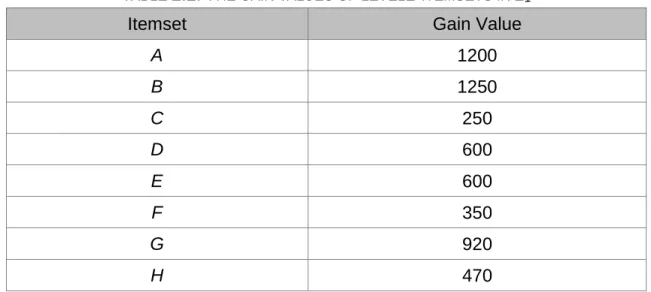
TABLE 2.2:THE GAIN VALUES OF LEVEL1-ITEMSETS IN L1
Itemset Gain Value
A 1200 B 1250 C 250 D 600 E 600 F 350 G 920 H 470
Step 5: These candidate erasable level 1-itemsets are then checked for whether
their gain values are smaller than or equal to the maximum gain threshold
T t, which is 2420 0.35= 847. In this example, the set of erasable level 1-itemsets includes {C}, {D}, {E}, {F} and {H} satisfy the condition and are then put into the erasable level 1-itemsets E1. The results are shown in
Table 2.3.
Table 2.3: The erasable level 1-itemsets with their gain values in E1
Itemset Gain Value
C 250
D 600
E 600
F 350
Step 6: The candidate erasable level 2-itemsets are then formed from the
erasable level 1-itemsets in E1. In this example, the following ten candidate
level 2-itemsets are generated: {CD}, {CE}, {CF}, {CH}, {DE}, {DF}, {DH}, {EF}, {EH} and {FH}.
Step 7: The varaibale k is then increased to 2.
Step8: In this example, since ten candidate erasable itemsets are generated in
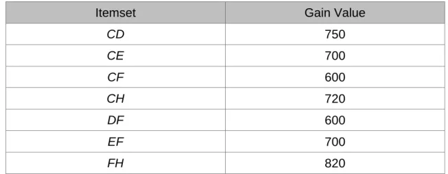
Step 6, Steps 4 to 7 are repeated as follows. The gain values of the ten candidate level 2-itemsets are calculated and compared with the maximum gain threshold in Steps 4 and 5. Take the 2-itemset {CD} as an example. Since all the products d3 to d8 contain at least C or D, the gain values of
these products are then added as the gain of {CD}, which is 750. The value is larger than the maximum gain threshold 847 and thus {CD} is a level 2-erasable itemset. The other candidate 2-itemsets can be processed in a similar way. Finally, the set of erasable 2-itemsets and the gain value are less than the threshold shown in Table 2.4.
Table 2.4: The gain values of the mined erasable level 2-itemsets in E2
Itemset Gain Value
CD 750 CE 700 CF 600 CH 720 DF 600 EF 700 FH 820
Then in Step 6, the only candidate erasable level 3-itemset, {CDF}, is generated and forms L3. The variable k then becomes 3 and Steps 4 to 7 are
executed again. The gain value of {CDF} is 750, smaller than the maximum gain threshold. Thus, it is an erasable itemset.
Step 9: All the erasable itemsets generated so far are output. The results are
TABLE 2.5:THE FINAL ERASABLE ITEMSETS IN THIS EXAMPLE Itemset Gain Value C 250 D 600 E 600 F 350 H 470 CD 750 CE 700 CF 600 CH 720 DF 600 EF 700 FH 820 CDF 750
CHAPTER 3
A Multiple Sources Data Mining
Algorithm for Mining Erasable
Itemsets
In this chapter, we will present the proposed approach for incrementally mining erasable itemsets. This chapter are organized as follows. The main idea about the proposed algorithm is described in Section 3.1. The notation used is listed in Section 3.2. The proposed TEIMA (Erasable Itemset- Multi-Sources Data Mining) erasable mining algorithm is stated in Section 3.3. Finally, an example for the proposed TEIMA erasable mining algorithm is given to explain the execution process in Section 3.4.
3.1 Main Idea
When companies or factories need to merge and the decision maker need to make decision to close some factories or stop some products in some factories, at first we are thinking about two factories merging and we can get the related individual factories EI data of those two factories, then split them to three item
sets as MEI, Q and R and do them with three cases:
Case 1: MEI set is including the all erasable itemset existing in both factories
product database and they are erasable for both factories, so for future merged factory that all items in MEI set will still be erasable items.
Case 2: Q set is including the erasable those just appear in the first factory (FPT1)
but not appear in the second factory (FPT2), for each item in Q set that its
erasable gain value from the first erasable itemset (EI1) is the gain value
from FPT1 then we no need to rescan the gain value again on FPT1 and
just need to scan it on FPT2 database to get its actual gain value then add
with the value from same item in EI1 then we can get the merged gain value
then compare with merged threshold value to see if it is erasable or not. It is easy to understand from META algorithm that will also can early remove the items in Q if it is non-erasable then its child item will also be erasable then more items can be skipped to scan the FPT2 database and reduce
more time spent.
Case 3: Same as Q set that R set is including the erasable those just appear in
the second factory (FPT2) but not appear in the first factory (FPT1), so for
itemset (EI2) is the gain value from FPT2 then we no need to rescan the
gain value again on FPT2 and just need to scan it on FPT1 database to get
its actual gain value then add with the value from same item in EI2 then we
can get the merged gain value then compare with merged threshold value to see if it is erasable or not. It is easy to understand from META algorithm that will also can early remove the items in R set if it is non-erasable then its child item will also be erasable then more items can be skipped to scan the FPT1 database and reduce more time spent.
3.2 The Terms
In this section, we introduce some concepts and terms that are used in this thesis.
Term 1: Factory Products Table (FPT):
The manufacturing company may own many different production factories those maybe locate on different countries, areas or cities places. They produce different products with different cost and gain values those we can list them as the Factory Products Table (FPT) for each production site or factory as follows:
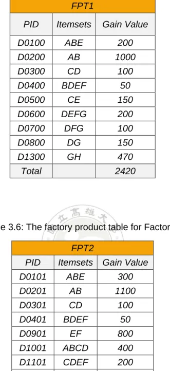
Table 3.1: Factory Products Table (FPT) from Factory 1 as FPT1.
FPT1
PID Itemsets Gain Value D0100 ABE 200 D0200 AB 1000 D0300 CD 100 D0400 BDEF 50 D0500 CE 150 D0600 DEFG 200 D0700 DFG 100 D0800 DG 150 D1300 GH 470 Total 2420
The PID stands for Product Identification. It is the ID for each different product that is made by different components. For example, in this case, product (ABE) is made by components A, B and E, and its PID is D01. For Factory 1, the product (ABE), its PID will plus factory ID (01) as D0101 lists in Factory 1’s FPT.
For same product and producing in different factories that base on different cost and profit, so that will have different gain value between different factories for same product.
For example, the gain value of item (ABE) in Factory 1 is 200 and 300 in Factory 2.
Term 2: Erasable Item sets (EI):
For each production factory that can be mined out its erasable item sets table that lists the erasable items with its gain value lower than the given threshold for individual site business analysis.
The EI is meaning that we can remove those EI components and products from the production line to meet the production down-sizing target and it can still keep operation with profitable. The EI table as below, EI1 that was mined from
Factory1 base on FTP1 bases on the threshold 35%.
Table 3.2: Erasable table from Factory1 as EI1.
EI1
Itemset Gain Value
C 250 D 600 E 600 F 350 H 470 CD 750 CE 700 CF 600 CH 720
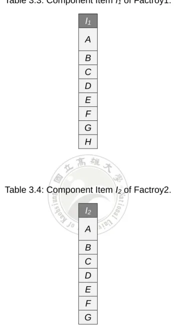
Term 3: Component item list (I) and Non-appear component item list (NI): The manufacturing factories are using different components lists for production, so there are some components different between factories, then for
Factory 1 (2) that we can get the component item (I) as,
Table 3.3: Component Item I1 of Factroy1.
I1 A B C D E F G H
Table 3.4: Component Item I2 of Factroy2.
I2 A B C D E F G
And from I1 and I2 that we can get the component H appears in I1 but not
in I2 then we define NI2 = {H} is the non-appear item for I2 compare to I1.
Problem Statement:
production scale downsizing, product class reducing or trading factories between companies. There is an issue/problem on how we can get the merged erasable item sets efficiently to figure out how arrange the production between operating sites to meet the business target. Here, we propose an efficient algorithm to get the merged EI and FPT efficiently for business decision making. The execution details of the proposed algorithm are described in the next section.
3.3 The Proposed Two-factory Erasable-itemset
Merging Algorithm (TEIMA)
In this section, the proposed two-factory erasable-itemset merging algorithm (TEIMA) is described in details. The whole algorithm is stated below: The Two-factory Erasable-itemset Merging Algorithm (TEIMA):
INPUT: A company with two factories, each of which has its own factory product
table (FPT) and total profit value (TP), a threshold ratio t for erasable itemsets, and the erasable itemsets (EI) in each factory.
OUTPUT: The merged erasable itemsets from the 2 factories.
Step 1: Initially set the final merged erasable set MEI as .
where TP1 and TP2 are the total profits of the two factories and t is the
threshold ratio.
Step 3: Find NI1 = I2 – I1, and NI2 = I1 – I2, where I1 and I2 are the sets of
components (items) appearing in Factories 1 and 2 respectively, NI1 is the
set of components (items) not appearing in Factory 1 but appearing in Factory 2, and NI2 is the set of components (items) not appearing in
Factory 2 but appearing in Factory 1.
Step 4: Divide the erasable itemsets in both EI1 and EI2 into the following three
cases:
Case 1: Set MEI = (EI1 ∩ EI2) ∪(EI1 ∩ NI2) ∪ (EI2 ∩ NI1), where each itemset
in MEI exists in both EI1 and EI2 and is certainly a final erasable
itemset.
Case 2: Set Q = (EI1 ∪ NI1) – EI2, where each itemset in Q exists in EI1 or
NI1 but not in EI2, and may or may not be a final erasable itemset.
Case 3: Set R = (EI2 ∪ NI2) – EI1, where each itemset in R exists in EI2 or
NI2 but not in EI1, and may or may not be a final erasable itemset.
Step 5: (for Case 1) Calculate the merged gain value of each itemset e ∈ MEI, which is a final erasable itemset, as follows:
Where e.GainValue1 and e.GainValue2 are the gain values of the
erasable itemset e in EI1 and EI2, respectively.
Step 6: Set k = 1, where k records the number of items in the itemsets currently being processed.
Step 7: (for Case 2). For each k-itemset e ∈ Q, which is an erasable k-itemset in EI1 but not in EI2, do the following sub-steps:
Step 7-1: Set its reduced itemset e’ = e - NI2;
Step 7-2: If e’ is , set the gain value of e’ in the second factory product table (FPT2) = 0; otherwise scan FPT2 to get the gain value of e’
in FPT2.
Step 7-3: For e’, to calculate the merged gain value of e as:
e.GainValue = e.GainValue1 + e’.GainValue2.
Step 7-4: Add e to MEI if e.GainValue is less than or equal the merged total profit value threshold (MT).
Step 8: (for Case 3) For each k-itemset e ∈ R, which is an erasable k-itemset in
EI2 but not in EI1, do the following sub-steps:
Step 8-1: Set its reduced itemset e’ = e - NI1.
Step 8-2: If e’ is , set the gain value of e’ in the first factory product table (FPT1) = 0; otherwise scan FPT1 to get the gain value of e’ in
FPT1.
Step 8-3: Calculate the merged gain value of e as:
e.GainValue = e.GainValue1 + e’.GainValue2.
Step 8-4: Add e to MEI if e.GainValue is less than or equal the merged total profit value threshold (MT).
Step 9: If k = 1, set NI1 = NI1 ∩ MEI1 and NI2 = NI2 ∩ MEI1, where MEI1 is the
1-itemsets in MEI. Step 10: Set k = k + 1.
Step 11: Generate the candidate k-itemsets Ck from MEIk-1, where MEIk-1 is the
(k-1)-itemsets in MEI.
Step 12: Remove from Q the k-itemsets which are not in Ck, and add the
k-itemsets in Ck to Q which contains at least one item in NI1 with the other
items not NI1 forming a (k-1)- itemset in Q. Set the gain value of the added
k-itemset = the gain value of the corresponding (k-1)-itemset in Q.
Step 13: Remove from R the k-itemsets which are not in Ck, and add the
k-itemsets in Ck to R which contains at least one item in NI2 with the other
items not NI2 forming a (k-1)-itemset in R. Set the gain value of the added
k-itemset = the gain value of the corresponding (k-1)-itemset in R.
results, otherwise, repeat Steps 7 to 14.
3.4 An Example of the Proposed Algorithm (TEIMA )
In this section, a simple example is given to show how the proposed algorithm can be easily and efficiently used to find out the merged erasable itemsets from a two-factory environment. Assume there is one company which owns two manufacture factories denoted as Factory 1 and Factory 2. Each factory has its own factory product table (FPT), which records the products it produces, the items (components) for manufacturing the products, and the values the products make. Assume the two factory product tables respectively for the two factories are shown in Table 3.5 and Table 3.6.
Table 3.5: The factory product table for Factory 1
FPT1
PID Itemsets Gain Value D0100 ABE 200 D0200 AB 1000 D0300 CD 100 D0400 BDEF 50 D0500 CE 150 D0600 DEFG 200 D0700 DFG 100 D0800 DG 150 D1300 GH 470 Total 2420
Table 3.6: The factory product table for Factory 2
FPT2
PID Itemsets Gain Value D0101 ABE 300 D0201 AB 1100 D0301 CD 100 D0401 BDEF 50 D0901 EF 800 D1001 ABCD 400 D1101 CDEF 200 D1201 AG 100 Total 3050
Assume the threshold of erasable itemsets for both the factories are 0.35. For Factory 1, the total values of the products are 2420. The value threshold for erasable itemsets is 2420*0.35, which is 847. The erasable itemsets for Factory1
can thus be obtained by the batch approach and the results are shown in Table 3.7.
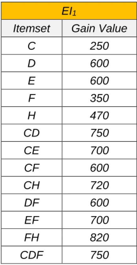
Table 3.7: The erasable itemsets obtained for Factory1
EI1
Itemset Gain Value
C 250 D 600 E 600 F 350 H 470 CD 750 CE 700 CF 600 CH 720 DF 600 EF 700 FH 820 CDF 750
Similarly, the total values of the products for Factory 2 are 3050. The value threshold for erasable itemsets is thus 3050*0.35, which is 1067.5. The erasable itemsets for Factory 2 are thus obtained as shown in Table 3.8.
Table 3.8: The erasable itemsets obtained for Factory 2
EI2
Itemset Gain Value
C 700 D 750 G 100 CD 750 CG 800 DG 850 CDG 850
With these individual data for the two factories, the decision makers at the headquarters may want to query about the final erasable itemsets when considering Factory1 and Factory 2 together. For this case, the proposed two-factory erasable-itemset merging algorithm (TEIMA) proceeds as follows.
Step 1: The final merged erasable set MEI is initially set as .
Step 2: Since the threshold ratio is 35%, the merged total profit value threshold (MT) is calculated as:
MT = (2420+3050)*0.35 = 5470*0.35 = 1914.5.
Step 3: The set of components (items) not appearing in Factory 1 but appearing in Factory 2, and the set of components (items) not appearing in Factory 2 but appearing in Factory1 are found. In this example, the set of components in the two factories are: I1 = {A, B, C, D, E, F, G, H} and I2 = {A,
Step 4: The erasable itemsets in both EI1 and EI2 are divided into the three cases
– MEI, Q and R as follows.
Case 1: MEI = (EI1 ∩ EI2)∪ (EI1 ∩ NI2) ∪ (EI2 ∩ NI1). The result is {{C}, {D},
{CD}} ∪ {{H}} ∪ , which is {{C}, {D}, {H}, {CD}}. The result with the gain values for the example is shown in Table 3.9. All these itemsets are certainly erasable after the merge.
Table 3.9: The itemsets in Case 1
MEI Itemset Gain Value in
FPT1 Gain Value in FPT2 C 250 700 D 600 750 F 350 1050 H 470 0 CD 750 750
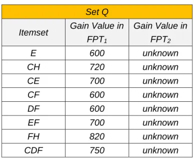
Case 2: Q = (EI1 ∪ NI1) – EI2, where each itemset in Q exists in EI1 or NI1
but not in EI2. The result for the example is shown in Table 3.10. All
Table 3.10: The itemsets in Case 2
Case 3: R = (EI2 ∪ NI2) – EI1, where each itemset in R exists in EI2 or NI2
but not in EI1. The result for the example is shown in Table 3.11. All
these itemsets are not certainly erasable after the merge.
Table 3.11: The itemsets in Case 3
Set R Itemset Gain Value in
FPT1 Gain Value in FPT2 G unknown 100 CG unknown 800 DG unknown 850 CDG unknown 850
Step 5: (for Case 1) the merged gain value of each itemset in MEI is calculated. Take the itemset {C} in MEI as an example. Its gain values in EI1 and EI2
Set Q Itemset Gain Value in
FPT1 Gain Value in FPT2 E 600 unknown CH 720 unknown CE 700 unknown CF 600 unknown DF 600 unknown EF 700 unknown FH 820 unknown CDF 750 unknown
are 250 and 700, respectively. Thus its merged gain value is (250+700), which is 950. The results for all the three itemsets in MEI are shown in Table 3.12. Note that all the five itemsets are erasable.
Table 3.12: The MEI table for Case 1
MEI C 950 D 1350 F 1400 H 470 CD 1500
Step 6: The variable k is set at 1, where k records the number of items in the itemsets currently being processed.
Step 7: (for Case 2) since k = 1, the merged gain values of the 1-itemsets in Q are to be found. In this example, there is one itemset including {E} in Q. In Sub-step 7-1, the itemsets to be checked become its reduced itemset as {E} – {H} = {E}. Since the gain value of {E} in the second factory product
table (FPT2) are unknown, FPT2 is scanned to get their gain values as 1350,
respectively. The merged gain values of the itemset is then calculated. Take the 1-itemset {E} as an example. Its final gain values can be calculated as
Since the gain value of {E}, which is 1950, is larger than the merged total gain value threshold (MT), which is 1914.5, {E} is thus non-erasable. Thus no erasable need to be added to MEI. The results of
MEI after the step are shown in Table 3.13.
Table 3.13: The MEI content after some 1-itemsets from Q are added.
Set MEI C 950 D 1350 F 1400 H 470 CD 1500
Step 8: The step is similar to Step 7, except handling R instead of Q. In this example, there is only one 1-itemset {G} in R. Since NI1 =, the itemset to
be checked is still {G}. The first factory product table (FPT1) is then
scanned to get the gain value of {G} in FPT1 as 920. The merged gain
value of {G} is then calculated as:
GainValue of {G} = 920 (GainValue1) + 100 (GainValue2) = 1020.
Since the gain value of {G} is smaller than MT, which is 1914.5, {G} is thus erasable and added to MEI. The results of MEI after the step are shown in Table 3.14.
Table 3.14: The MEI content after {G} from R is added. MEI C 950 D 1350 F 1400 G 1020 H 470 CD 1500
Step 9: Since k = 1, NI1 = NI1∩MEI1 = and NI2 = NI2∩MEI1 = {H}, where MEI1 is
the 1-itemsets in MEI. The MEI1 shown in Table 3.15.
Table 3.15: The MEI1 content.
Set MEI1 C 950 D 1350 F 1400 G 1020 H 470
Step 10: The current k value becomes 1+1, which now is 2.
Step 11: The candidate 2-itemsets C2 are then generated from MEI1. They include
{CD}, {CF}, {CG}, {CH}, {DF}, {DG}, {DH}, {FG}, {FH}, {GH}, which have all their 1-sub-itemsets in MEI1.
there are six 2-itemsets including {CH}, {CE}, {CF}, {DF}, {EF} and {FH} in
Q. Among them, {CE} and {EF} are not in C2 and are thus removed from
Q. Then the 2-itemsets in C2 which contains at least one item in NI 1 with
the other items not NI1 forming a 1-itemset in Qare added to Q. In this
example, since NI1=, thus no itemset is added to Q. The result of the set
Q after this step are shown in Table 3.16.
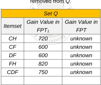
Table 3.16: The content of Q after some unpromising 2-itemsets are removed from Q.
Set Q Itemset Gain Value in
FPT1 Gain Value in FPT CH 720 unknown CF 600 unknown DF 600 unknown FH 820 unknown CDF 750 unknown
Step 13: Similar to Step 12, the 2-itemsets in R which are not in C2 are removed.
In this example, there are two 2-itemsets including {CG} and {DG} in R. Since both of them are in C2, they are not removed from R. Then the
2-itemsets in C2 which contains at least one item in NI
and {CH}, {DH}, {FH} and {GH} include the item H. {CH} is then first processed. The remaining item of the itemset {CH} is C, which does not exist (i.e. not erasable) in R. Thus, {CH} is not added to R. Similarly, {FH} is not added to R, but {DH} and {GH} are added to R. The gain values of {DH} and {GH} are equal to those of the corresponding 1-itemsets {D} and {G} in R. The results of the set R after this step are shown in Table 3.17.
Table 3.17: The content of R after Step 13 is executed.
Set R Itemset Gain Value in
FPT1 Gain Value in FPT2 CG unknown 800 DG unknown 850 DH unknown 750 (=D) GH unknown 100 (=G) CDG unknown 850
Step 14: Since there still are 2-itemsets in both Q and R, then we process Step 7 with k=2 and NI2 = {H}, then we scan {CH}, {CF}, {DF} and {FH} in FPT2 as
Table 3.18: The content of Q after 2-itemsets scan in FPT2.
Set Q Itemset Gain Value in
FPT1 Gain Value in FPT2 CH 720 700 CF 600 1550 DF 600 1550 FH 820 1050 CDF 750 unknown
And calculate their merged gain values as {CH} is 1420 that is smaller than MT, then we need to add it to MEI since it is 2-itemset erasable itemset. Similarly, {FH} is 1870 is smaller than MT that also need to be added to MEI. But for {CF} and {DF}, their merged gain values are larger than MT are non-erasable itemsets then we no need to add them to MEI. After Step 12 the set MEI shown as Table 3.19.
Table 3.19: The MEI content after 2-itemset with Step 7.
MEI C 950 D 1350 F 1400 G 1020 H 470 CD 1500 CH 1420 FH 1870
For set R, also follow Step 8-1 and Step 8-2 scan on FPT1 and get the
result as Table 3.20.
Table 3.20 The R content after follow Step 8-1 to Step 8-2 for k= 2
Set R Itemset Gain Value in
FPT1 Gain Value in FPT2 CG 1170 800 DG 1070 850 DH 1070 750 (=D) GH 920 100 (=G) CDG unknown 850
Then add {GH} and {DH} itemsets to MEI since their gain values are less than 1914.5 (MT) and the MEI result as Table 3.21.
Table 3.21: The MEI after Step 8 for k= 2
MEI C 950 D 1350 F 1400 G 1020 H 470 CD 1500 CH 1420 DH 1820 FH 1870 GH 1020
Then repeat Step 10 to Step 14 since there are 3-itemsets in Set Q and Set R.
Step 10: The current k value becomes 2+1, which now is 3.
Step 11: The candidate 3-itemsets C3 are then generated from MEI2. And it just
has only one itemset as {CDH} since others itemsets like {CDF} it is child itemset of {DF} that is non-erasable itemset then we no need to generate it for scan it.
Step 12: To remove {CDF} from set Q since it did not appear in C3. Then no
3-itemset or above 3-itemset in set Q.
Step 13: Same with Step 12 that we also can remove {CDG} from set R but we need to add {CDH} into set R since it includes {H} as the NI2 and the set R
shown as Table 3.22.
Table 3.22 The R content after follow Step 13 with k= 3
Set R Itemset Gain Value in
FPT1 Gain Value in FPT2 G 920 100 CG 1170 800 DG 1070 850 DH 1070 750 (=D) GH 920 100 (=G) CDH unknown 750 (=CD)
process Step 8 and get the gain value of {CDH} is 1220+750 = 1970 is larger than MT then we no need to add it to MEI.
Step 10: Set k = 3+1 which now is 4.
Step 11: Since there is no 3-itemset in MEI then no MEI4 can be generated and
same for C4.
Step 12: Since there is no 4-itemset in set Q then stop processing Step 12. Step 13: Since there is no 4-itemset in set R then stop processing Step 13. Step 14: No 4-itemset or above itemset in both Q and R then output MEI as the
final result and shown in Table 3.23.
Table 3.23: The final results of the MEI content.
MEI C 950 D 1350 F 1400 G 1020 H 470 CD 1500 CH 1420 DH 1820 FH 1870 GH 1020
3.5 The Proposed Multiple-factory
Erasable-itemset Merging Algorithm (MEIMA)
In this section, the proposed multiple-factory erasable-itemset merging algorithm (MEIMA) is described in details. The whole algorithm is stated below:
The Multiple-factory Erasable-itemset Merging Algorithm (MEIMA):
INPUT: A company has multiple factories, each of which has its own factory
product table (FPT) and total profit value (TP), a threshold ratio t for erasable itemsets, and the erasable itemsets (EI) in each factory, and I is the all components set the using by all its factories.
OUTPUT: The merged erasable itemsets from those multiple factories.
Step 1: Initially set the final merged erasable set MEI as .
Step 2: Calculate the merged total profit value threshold (MT) as (TP1+TP2+…….
+ TPm)*t, where TP1, TP2 and TPm are the total profits of those factories
and t is the threshold ratio.
Step 3: I is the set of components (items) those appearing around all factories, it is components list for company level. To find components NI1 = I – I1, NI2
(items) appearing in Factories 1, 2 and m respectively, NI1 is the set of
components (items) not appearing in FPT1, and same for NI2 …. NIm.
Step 4: Union 1-itemset of all the erasable itemsets in EI1, EI2 …. EIm and NI1,
NI2 …. NIm and set the result as 1-EI.
Step 5: For each 1-itemset e ∈ 1-EI, there three conditions to set e.EIi.GainValue:
1. Set e.EIi.GainValue = gain value of e, if e exists in EIi or
2. Set e.EIi.GainValue = 0 if e ∈ NIi or
3. Scan e on FPTi to get the e.EIi.GainValue
Then, the merged gain value of e can be got by summing all
e.EIi.GainValue as,
𝑒. 𝐺𝑎𝑖𝑛𝑉𝑎𝑙𝑢𝑒 = ∑𝑚𝑖=1𝑒. 𝐸𝐼𝑖. 𝐺𝑎𝑖𝑛𝑉𝑎𝑙𝑢𝑒
For each 1-itemset e ∈ 1-EI, we can add e to MEI if its gain value is less than the merged total profit value threshold (MT).
Step 6: Set k = 2, where k records the number of items in the itemsets currently being processed.
Step 7: To generate all k-itemset from (k-1)-itemset in MEI by the Generating
candidate itemsets of META algorithm [3] and for each e ∈ k-EI, there four conditions to set e.EIi.GainValue:
1. If any component of e ∉ any NIi and e also does not appear in any EIi
then that is meaning e is nonerasable itemset in all FPTi, so we can
just remove e without any process.
2. Set e.EIi.GainValue = gain value of e, if e exists in EIi or
component of e ∈ NIi and (e - NIi) exists in EIi or
4. Scan e on FPTi to get the e.EIi.GainValue
Then, the merged gain value of e can be got by summing all
e.EIi.GainValue as,
𝑒. 𝐺𝑎𝑖𝑛𝑉𝑎𝑙𝑢𝑒 = ∑𝑚𝑖=1𝑒. 𝐸𝐼𝑖. 𝐺𝑎𝑖𝑛𝑉𝑎𝑙𝑢𝑒
Here for each k-itemset e ∈ k-EI, we can add e to MEI if its gain value is less than the merged total profit value threshold (MT).
Step 8: To check if any (k+1)- itemsets can be generated from k-itemsets in MEI by using the Generating candidate itemsets of META algorithm [3], if none can be generated then end the process and output MEI as the final result else set k=k+1 and repeat Step 7 to 8.
3.6 An Example of the Proposed Algorithm (MEIMA )
In this section, a simple example is given to show how the proposed algorithm can be easily and efficiently used to find out the merged erasable itemsets from a multiple–factory environment. Assume there is one company
which owns three manufacture factories denoted as Factory 1, Factory 2 and Factory 3. Each factory has its own factory product table (FPT), which records the products it produces, the items (components) for manufacturing the products, and
the values the products make. Assume the two factory product tables respectively for the two factories are shown in Tables 3.24, 3.25 and 3.26.
Table 3.24: The factory product table for Factory 1
FPT1
PID Itemsets Gain Value D0100 ABE 200 D0200 AB 1000 D0300 CD 100 D0400 BDEF 50 D0500 CE 150 D0600 DEFG 200 D0700 DFG 100 D0800 DG 150 D1300 GH 470 Total 2420
Table 3.25: The factory product table for Factory 2
FPT2
PID Itemsets Gain Value D0101 ABE 300 D0201 AB 1100 D0301 CD 100 D0401 BDEF 50 D0901 EF 800 D1001 ABCD 400 D1101 CDEF 200 D1201 AG 100 Total 3050
Table 3.26: The factory product table for Factory 3
FPT3
PID Itemsets Gain Value D3100 AB 300 D3200 ABD 350 D3300 AEF 400 D3400 BG 800 D3500 EF 150 D3600 ADG 200 D3700 DFG 100 D3800 DGE 450 D3300 ADFG 400 Total 3150
Assume the threshold of erasable itemsets for both the factories are 0.35. For Factory 1, the total values of the products are 2420. The value threshold for erasable itemsets is 2420*0.35, which is 847. The erasable itemsets for Factory1 can thus be obtained by the batch approach and the results are shown in Table 3.27.
Table 3.27: The erasable itemsets obtained for Factory1 EI1 Itemset Gain Value C 250 D 600 E 600 F 350 H 470 CD 750 CE 700 CF 600 CH 720 DF 600 EF 700 FH 820 CDF 750
Similarly, the total values of the products for Factory 2 are 3050. The value threshold for erasable itemsets is thus 3050*0.35, which is 1067.5. The erasable itemsets for Factory 2 are thus obtained as shown in Table 3.28.
Table 3.28: The erasable itemsets obtained for Factory 2 EI2 Itemset Gain Value C 700 D 750 G 100 CD 750 CG 800 CH 700 DG 850 DH 750 CDG 850
Similarly again, the total values of the products for Factory 3 are 3150. The value threshold for erasable itemsets is thus 3050*0.35, which is 1102.5. The erasable itemsets for Factory 3 are thus obtained as shown in Table 3.29.
Table 3.29: The erasable itemsets obtained for Factory 3
EI3 Itemset Gain Value E 1000 F 1050
With these individual data for the three factories, the decision makers at the headquarters may want to query about the final erasable itemsets when
considering Factory1, Factory 2 and Factory 3together. For this case, the proposed multiple-factory erasable-itemset merging algorithm (MEIMA) proceeds as follows.
Step 1: Initially set the final merged erasable set MEI as .
Step 2: Since the threshold ratio is 35%, the merged total profit value threshold (MT) is calculated as:
MT = (2420+3050+3150)*0.35 = 8620*0.35 = 3017.
Step 3: Find components NI1 = I – I1 =, NI2 = I – I2 = {H} and NI3 = I – I3 = {C, H}.
Step 4: Union 1-itemset of all the erasable itemsets in EI1, EI2 and EI3 and NI1,
NI2 and NI3 and set the result as 1-EI as Table 3.30.
Table 3.30: The 1-EI table from Step 4 1-EI EI1 EI2 EI3 Merged Itemset Gain Value Gain Value Gain Value Gain Value C D E F G H
Step 5: For {C} in 1-EI, we can get gain value 250 from EI1 and 700 from EI2, since
set the gain value as zero.
For {D} in 1-EI, we can get gain value 600 from EI1 and 750 from EI2, since
{D} exists in EI1 and EI2. For EI3, {D} ∉ NI3 then we need scan {D} on FPT3
to get its gain value as 1500.
Similar process for the rest 1-itemsets to get their gain value and merged gain value of each itemset as Table 3.31.
Table 3.31: The 1-EI table from Step 5 1-EI
EI1 EI2 EI3 merged
Itemset Gain Value Gain Value Gain Value Gain Value
C 250 700 0 950 D 600 750 1500 2850 E 600 1350 1000 2950 F 350 1050 1050 2450 G 920 100 1950 2970 H 470 0 0 470
And the gain values of {C}, {D}, {E}, {F}, {G} and {H} are all less than 3017 (MT) then need to add into MEI as Table 3.32.
Table 3.32: The MEI table from Step 5 MEI C 950 D 2850 E 2950 F 2450 G 2970 H 470
Step 6: Set k = 2, where k records the number of items in the itemsets currently being processed.
Step 7: To generate all 2-itemset as 2-EI from 1-itemset in MEI and the result as Table 3.33.
Table 3.33: The 2-EI table 2-EI
EI1 EI2 EI3 merged
Itemset Gain Value Gain Value Gain Value Gain Value
CD CE CF CG CH DE DF DG DH EF EG EH FG FH GH
For {CD} in 2-EI, we can get gain value 750 from EI1 and 750 from EI2,
since {CD} exists in EI1 and EI2. For EI3, {C} ∈ NI3 then we set the gain
value as 1500 same as the gain value of {D} since it exists in EI3.
For {CH} in 2-EI, we can get gain value 720 from EI1 and 700 from EI2,
since {CH} exists in EI1 and EI2. For EI3, {C, H} ∈ NI3 then we set the gain
value as zero same as the gain value of since {C, H} not exists in EI3.
For {DF} in 2-EI, we can get gain value 600 from EI1 since {DF} exists in
EI1 but for EI2 and EI3, {D, F} ∉ NI2 or NI3 then we need to scan {DF} on
FTP2 and FPT3 to get the gain values as 1150 and 2050.
For {DE} in 2-EI, it does not exist in EI1, EI2 and EI3 and {D, E} ∉ NI1, NI2
and NI3 then that is meaning they are all non-erasable itemset so we no
need to scan it on FPT and just remove it.
Similar process for the rest 2-itemset to get their gain value and merged gain value of each itemset as Table 3.34.
Table 3.34: The 2-EI table from Step 7 2-EI
EI1 EI2 EI3 Merged
Itemset Gain Value Gain Value Gain Value Gain Value
CD 750 750 1500 3000
CE 700 1850 1000 3550
CF 600 1550 1050 3200
CG 1170 800 1950 3920
CH 720 700 0 1420
DE nonerasable nonerasable nonerasable removable
DF 600 1550 2050 4200
DG 1070 850 2300 4220
DH 1070 750 1500 3320
EF 700 1350 1500 3550
EG nonerasable nonerasable nonerasable removable
EH 1070 1350 1000 3420
FG nonerasable nonerasable nonerasable removable
FH 820 1050 1050 2920
GH 920 100 1950 2970
And the gain values of {CD}, {CH}, {FH}, and {GH} are less than 3017 (MT) then need to add into MEI as Table 3.35.
Table 3.35: The MEI table from Step 7 MEI C 950 D 2850 E 2950 F 2450 G 2970 H 470 CD 3000 CH 1420 FH 2920 GH 2970
Step 8: To check the 2-itemsets in MEI, there are {CD}, {CH}, {FH}, and {GH} itemsets and by using the Generating candidate itemsets of META and they cannot generate any 3-itemset candidate itemset so the process stop and output the MEI as final MEI for FPT1, FPT2 and FPT3 merged erasable
itemsets shows in Table 3.36.
Table 3.36: The MEI table from Step 8
MEI C 950 D 2850 E 2950 F 2450 G 2970 H 470 CD 3000 CH 1420 FH 2920
CHAPTER 4
Experiments and Analysis
4.1
Experimental Environments
In this chapter, a series of experiments was conducted to evaluate the performance of the proposed TEIMA and MEIMA algorithm execution efficiency. All of the experiments were implemented in Visual C# 2015 and executed on an Apple MACBOOK with Window 10, 2.7 GHz CPU and 4 GB of memory.
The proposed TEIMA and MEIMA algorithm were run to compare their performance with META algorithm.
4.2 Experimental Settings
In the experiments, a program named “DataMaker” was used to produce the
required datasets.
The database detail as below:
1. Components in use: letters A~Z total 26 components.
3. Gain Value: 100 ~ 1500. 4. The threshold ratio is 45%.
4.3
Experimental Results
In this section, the experimental comparison between the previous META algorithm and the proposed TEIMA and MEIMA are described.
4.3.1 Experiment 1 Results on two factories
merged with same product items number
The first experiment evaluates the effect of merging two factories those factories has same products item numbers as 100, 250, 500, 1000 and 10000 product items for each one factory.
Figure 4.1 shows the execution time required by the two algorithms which process two merging factories with 100, 250 and 500 product items and Figure 4.2 shows result for product items are 1000 and 10000.
Figure 4.1: Results of two factories with 100, 250 and 500 product items settings
Figure 4.2: Results of two factories with 1000 and 10000 product items settings
From the figures show the TEIMA spent less time to complete the merged erasabel itemsets (MEI) mining so the run time performance is better than
META. That is making sense since TEIMA scans few less database than META
that cause time spent different.
0 0.5 1 1.5 2 2.5 3 3.5 4 100 250 500
Experiment 1
META TEIMA Run T im e (se c.) 0 100 200 300 400 500 600 700 800 900 1000 10000Experiment 1
META TEIMA Run T im e (se c.)4.3.2 Experiment 2 Results on two factories
merged with different product items number
The second experiment evaluates the effect of merging two factories those factories have different products item numbers as Factory 1 has 100 product items and merged with as Factory 2 has 500 product items, or Factory 1 has 100 product items merged with Factory 2 has 1000 product items which one small database merged with another larger database.
Figure 4.3 and Figure 4.4 show the execution time required by the two algorithms for processing for two merging factories with D1 (100 items merged with 500 items), D2 (100 items merged with1000 items) , D3 (100 items merged with 10000 items).
Figure 4.3: Results of two factories with D1 and D2 database settings
0 0.5 1 1.5 2 2.5 3 3.5 D1 D2
Experiment 2
META TEIMA Run T im e (Sec.)Figure 4.4: Results of two factories with D2 and D3 database settings
From the result of experimental 2 shows the TEIMA still spent few less time to complete the merged erasable itemsets (MEI) mining.
4.3.3 Experiment 3 Results on multi-factories with
different product items number
The 3rd experiment were made to evaluate the multi-factories as ten
factories merging with difference product items number per factory as 250, 500, 1000 and 10000 product items for each factory. The Figure 4.5 shows the execution time required by the MEIMA and META algorithms for processing.
0 50 100 150 200 250 300 350 400 450 D2 D3