An Application of the Empirical-Distribution-Based Model on the Implied Volatility of Taiwan Warrants

全文

(1)An Application of the Empirical-Distribution-Based Model on the Implied Volatility of Taiwan Warrants Chyong Ling Chen*. Theories such as jump process, stochastic volatility, the GARCH model, and implied risk-neutral distribution have been developed to account for the volatility smile. Nevertheless, none of them succeeds in solving the smile problem. A newly creative empirical-distribution-based model (EDB model) which uses a histogram constructed from past asset prices has been applied to the S&P 500 index and it eliminates the degree of smile and the price difference. This study applies the same methodology on the TSM and UMC call warrants on the Taiwan stock market to compare its pricing and volatility smile with those derived from the Black-Scholes model. The results show that the degree of smile is not as great in the EDB model with a long historical horizon as in the BS model. Using the average value of the implied volatility as a standard deviation, the fitted prices were computed. The actual option price and both the fitted prices from the BS model and EDB model are all overpriced after examining the sell-naked profit. The profit from the EDB model is lower than the profit from the BS model and from the actual market price. This overpricing is more serious for the in-the-money than the out-of-the-money warrants and is less serious if longer historical data is used. Keywords：Warrants, Implied Volatility, Volatility Smile, Histogram.. _______________________________________________________________________ * Associate Professor, Department of Economics, Feng Chia University, 100 Wen Hwa Road, Taichung, Taiwan. E-mail: clchen@fcu.edu.tw. 1. 第五屆全國實證經濟學論文研討會 The 5th Annual Conference of Taiwan's Economic Empirics.

(2) 台灣認購權證隱含波動的探討─實質分配模型的應用陳瓊怜* 許多理論模型，諸如跳躍過程、隨機波動、GARCH 模型和隱含中性風險分配模型等，已被發展出來因應隱含波動的問題。然而沒有一個成功地解決了波動微笑(volatility smile)的問題。利用過去資產歷史價格的統計圖表(histogram)所建構出的所謂實質分配模型(EDB model)，應用在 S&P 500 指數可減低微笑的程度和理論價格與市場價格的差距。EDB model 是一個創新的模型，已有多個應用此模型在債券和其它選擇權的研究正在進行中。本文應用修正過的 EDB model 在台灣股票市場的台積電與聯電認購權證上，以比較在波動微笑與價格差距上 EDB model 與 Black-Scholes model 的異同。研究結果發現，若使用長歷史水平的資產價格為基礎，則 EDB model 所導出的微笑幅度比 Black-Scholes model 的小。以隱含波動的平均值當做標準差來計算權證的理論適配值，結果發現依 EDB model 和 Black-Scholes model 所計算出的理論適配值與實際市場價格皆呈現價格過高的現象。由 EDB model 的理論適配值所得到的裸售利潤比其他二者低。這種超額利潤的現象價內權證比價外權證嚴重；同時使用短歷史水平的資產價格比使用長歷史水平的資產價格所計算出的理論適配值，其超額利潤也較高。. 關鍵詞：認購權證、隱含波動、波動微笑、歷史價格的統計圖。. _______________________________________________________________________ * 逢甲大學經濟系副教授. 2. 第五屆全國實證經濟學論文研討會 The 5th Annual Conference of Taiwan's Economic Empirics.

(3) 1. Introduction Since the introduction of the Black-Scholes model (1973), researchers have studied the empirical performance of the model. Early studies find that after comparing market prices and predicted prices, the model systematically miscalculates (or biases) the impact of strike prices on option prices. Starting in the early 1990’s, researchers focused on the corresponding biases in implied volatility. The strike price bias, termed “volatility smile,” considers the relationship between strike prices and implied volatility. The volatility smile that is generated by the Black-Scholes model can be attributed to either of the following reasons. First, the normality assumption of the return distribution of the underlying asset is inappropriate. Second, in- and/or out-of-the-money options are indeed overpriced. Several studies attempted to resolve the strike biases in implied volatility by introducing different specifications into the distribution of the underlying asset to account for the fat tail phenomenon. Those specifications included the jump-diffusion ( Naik and Lee 1990 and Bates 1991), stochastic volatility (Hull and White 1987, Johnson and Shanno 1987, Wiggins 1987, Heston 1993, Ritchen and Trevor 2000), combined jumps and stochastic volatility (Scott 1997, and Bakshi, Cao, and Chen 1997), implied risk neutral distribution (Shimko 1993, Derman and Kani 1994, Dupire 1994, Rubinstein 1994), GARCH process ( Duan 1995, Kallsen and Taqqu 1998, Ritchen and Trevor 2000), and hyperbolic distribution (Eberlein, Keller, and Prause 1998). Some researchers even attributed the smile to the non-fundamental factors of the market (Longstaff (1995) Jackwerth and Rubinstein (1996), Dumas et al. (1998), Pena et al. (1999)). However, Das and Sundaram (1999) indicated that incorporating these features mitigated, but did not eliminate, the smile. Instead of proposing a theoretical return distribution, Chen and Palmon (2002) hypothesized that traders priced options using historical return distribution. Hence, they constructed a histogram from past S&P 500 daily returns and used it to price S&P 500 options. They found that their empirical-distribution-based model (EDB model) predicted option premiums considerably better than the Black-Scholes model (BS model) and it successfully eliminated the smile for the in-the-money options. They also found that out-of-the-money options were overpriced. In this study, the same methodology was applied on the call warrants in the Taiwan stock market. First, the implied volatility was computed by the BS model and the EDB model. Using the average value of the implied volatility as a standard deviation, the fitted prices were computed. Then the problem of overpricing was examined by checking the sell-naked profit of the fitted price and the actual price. The organization of this paper is as follows. In section 2, the warrants under study were explained and the related studies were reviewed. In section 3, the implied volatility and the fitted prices using both the BS model and the EDB model were computed. Also the volatility smile was checked and the sell-naked profit was calculated. Concluding remarks are given in section 4, and the EDB model is explained in the appendix.. 3. 第五屆全國實證經濟學論文研討會 The 5th Annual Conference of Taiwan's Economic Empirics.

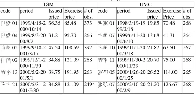
(4) 2. Warrant in this study The first warrant on the Taiwan stock market was offered on September 4, 1997. Warrants were issued by brokerage firms and traded in the stock market. By the end of 2000, 126 warrants had been issued. All warrants in the market are call warrants. Put warrants are not permitted. Among the call warrants, 110 have a single stock as its underlying asset and 16 have mixed stocks as its underlying asset. Among the former, 8 warrants have Taiwan Semiconductor Manufacturing (symbol: TSM) as their underlying asset while 6 warrants have United Microelectronics (symbol: UMC). Overall, those two are the most popular warrants in the market. In addition, the ADR of the TSM and the UMC are listed in New York Stock Exchange (NYSE). Due to the similarity of these companies and their exposure to the international market, their warrants have been chosen for analysis in this study. All of the warrants expire in one year except for two –Jihsun 01 and Kingwha 02 that cover a year and half. Fubon 10 and Polaris 16 were dropped due to an incomplete data set since they were issued at the end of November 2000. Therefore, a total of 12 warrants are included in this study, 6 each for TSM and UMC. Table 1 shows the details of the warrants under study. Total observations are 1811 for TSM and 1600 for UMC. The warrant in the Taiwan stock market is an American option. Yet, since the strike price is adjusted when the dividend is distributed and there is a tax disadvantage1 on early exercise, investors usually do not exercise the warrants before the expiration date. These properties make the warrant European style. Investors can realize a profit by selling the warrant in the market. So far, the pricing models discussed in the articles relating to the Taiwan warrants are limited to the Black-Scholes model (俞明德等 1999，李怡宗等 1999，施東河、王勝助 2001), the jump-diffusion model (俞明德等 1999，林丙輝、王明傳 2001), the CEV model (徐宗德等 1998，詹錦宏等 1999), binomial model (許溪南、張博彥 2002), and the GARCH model (巫春洲 2002). Although a few papers studied implied volatility (李進生等 2000，俞明德等 1999), they all use Black-Scholes formula to derive the option prices. 李進生等 (2000) examined the forecasting power of the five models which adopted historical volatility, Black-Scholes implied volatility, and ARCH, GARCH and random walk volatility in the model. Using the 16 warrants from September 1997 to March 1999, they found that the historical volatility model had better forecasting power than the implied volatility model. 李怡宗等(1999) had tried to find the factors which caused the difference between the market price and the theoretical price. The BS model was used to derive the theoretical price. The results showed that the Black-Scholes implied volatility affected the difference significantly. These two and other articles indicated that the Black-Scholes implied volatility was overvalued. Yet, no article has proven or discussed the presence or absence of a volatility smile.. 1. Refer to 楊淑卿(2003).. 4. 第五屆全國實證經濟學論文研討會 The 5th Annual Conference of Taiwan's Economic Empirics.

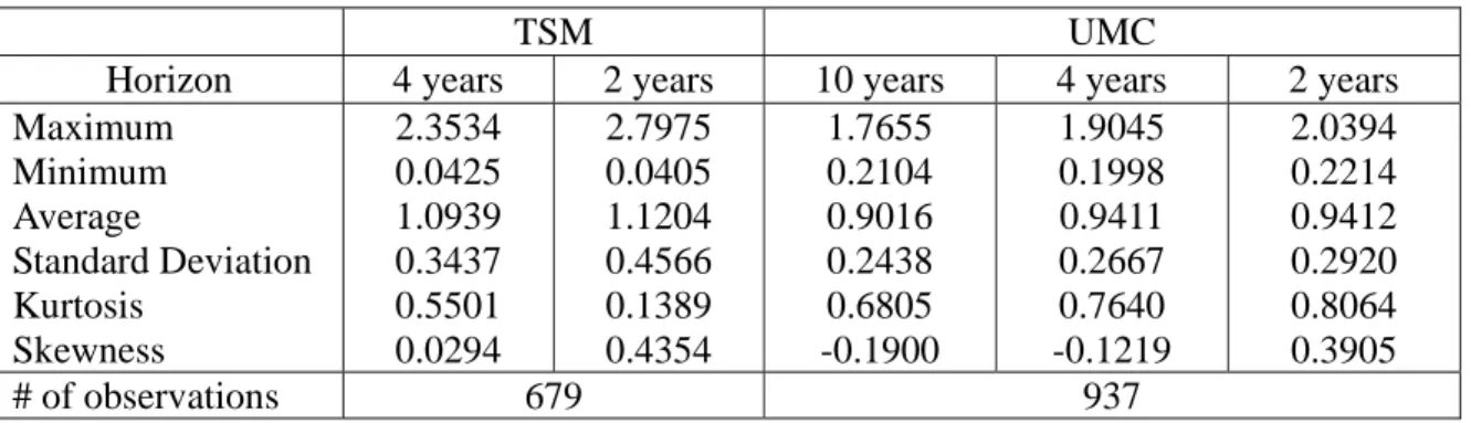
(5) 3. The empirical results In the BS model, one of the assumptions is that the underlying asset does not yield a dividend. Both TSM and UMC traditionally distributed dividends every year and the strike price is adjusted for the dividend. For example, if the ex-dividend date is on 5/9/ 2000 for the UMC stock and the dividend rate is 20%, therefore, the stock price and strike price would be both adjusted by 20% on 5/10/2000. Under this situation, the traditional BS model was applied to the Taiwan warrant as if it is a European option. In this study, the historical stock prices used to construct a histogram for TSM are from 1994/9/5 to 2001/5/11 covering 1846 data set and for UMC are from 1986/11/06 to 2001/5/11 covering 4461 data set. 1994/9/5 and 1986/11/06 are the dates when TSM and UMC stocks respectively went public. Both price series had been adjusted to the dividend rate every year. The summary statistics of TSM and UMC stock prices are shown in Table 2. Table 2 shows that the average daily return and standard deviation are 0.17% and 0.0269 for TSM stock while they are 0.16% and 0.0283 for UMC stock. Two important characteristics of these historical distributions have been noted. First, the return distributions present fat tails (extra kurtosis). Second, the extra kurtosis decreases as the holding period lengthens. Using the BS model, implied volatility (σBS) for both warrants2 was computed. For TSM, 1132 out of a total of 1811 observations (62.51%), the calculated implied volatility is 0. For UMC, 663 out of a total of 1600 observations (41.44%), the calculated implied volatility is 0. This implies that the actual warrant prices are lower than their intrinsic values- an obvious arbitrage opportunity. This happens in the sample probably because the daily warrant and stock prices are not synchronized. This non-synchronization can be attributed to the low liquidity and the weak-form efficient market in Taiwan3. Although, deleting these observations may result in a selection bias in favor of observations with a relatively high implied volatility, these observations were dropped since the ratios were so high. The data left for further study is 679 for TSM and 937 for UMC. The distribution of the moneyness of these two warrants is listed in Table 3. Table 3 shows that 163 observations are in-the-money and 516 observations are out-of-the-money for TSM while 152 observations are in-the-money and 785 observations are out-of-the-money for UMC. In the next step, the implied volatility, σEDB, from the EDB model was derived for the remaining data. The volatility in this model were allowed to vary but other moments are kept fixed. Using the model described in the appendix, the implied volatility using the past historical specification of the distribution was generated. Two time horizons, 4 years and 2 years, for TSM and 3 time horizons, 10 years, 4 years and 2 years, for UMC4 were chosen. The summary statistics of both implied volatility, σBS and σEDB, are presented in 2. Price of warrants and stocks is from the Taiwan Economic Journal data bank. Interest rate is 90 days bank rate from AREMOS data bank. 3 The trading volume of warrants in Taiwan is usually much smaller than that of stocks. Also, the brokerage firms did not perform well as a market maker even when the liquidity is very low or zero. 4 Stock of TSM went public on 9/5/1994 and its first warrant was traded on 4/5/1999. Therefore its maximum historical horizon was 4.5 years.. 5. 第五屆全國實證經濟學論文研討會 The 5th Annual Conference of Taiwan's Economic Empirics.

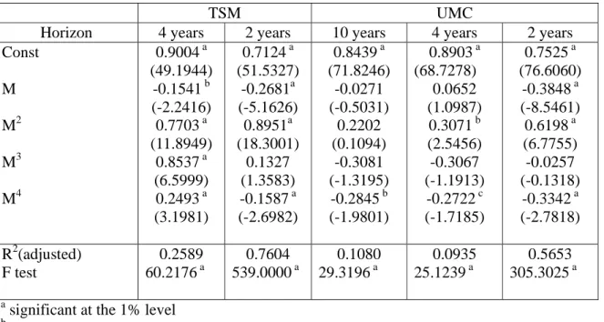
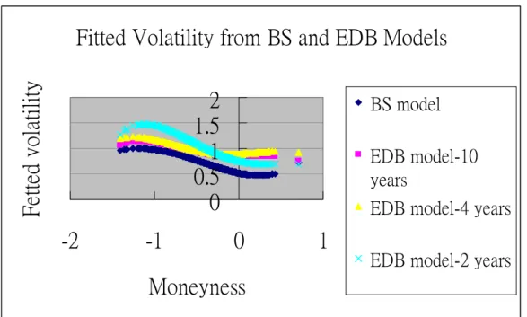
(6) Table 4 and 5, respectively. Table 4 shows that the average volatility and its standard deviation of σBS are 0.6333 and 0.2604 for TSM warrants and are 0.6578 and 0.2055 for UMC warrants. Table 5 shows that the average volatility and its standard deviation of σEDB are 1.0939 and 0.3437 for a 4 year horizon and 1.1204 and 0.4566 for a 2 year horizon for TSM warrants. These data are 0.9016 and 0.2438 under 10 year horizon, 0.9411 and 0.2667 for a 4 year horizon, 0.9412 and 0.2920 for a 2 year horizon for UMC warrants. It can be seen that the longer the horizon the smaller the average and standard deviation of the σEDB. To examine the smile problem, the following regressions were employed:. ⎧⎪σˆ BS = a + b1 M + b2 M 2 + b3 M 3 + b4 M 4 + e ⎨ ⎪⎩σˆ EDB = a + b1 M + b2 M 2 + b3 M 3 + b4 M 4 + e. (1). where σˆ BS and σˆ EDB are the annualized implied volatilities derived from the BS model and the EDB model, respectively. The variable M is the moneyness, which is defined as M = ( S − K ) / S . The third and fourth powers of the moneyness measure were included in our regressions so not to restrict the quadratic shape of the smile. The estimates from the regression were presented in Table 6 and 7. Table 6 shows that the b2s, the coefficients of M2 in the σˆ BS equation, are 0.8897 for TSM and 0.5347 for UMC. Table 7 shows that the coefficients in the σˆ EDB are 0.7703 and 0.8951 for 4 year horizon and 2 year horizon respectively for TSM warrants, while they are 0.2202, 0.3071 and 0.6198 for 10 year, 4 year and 2 year horizon respectively for UMC. In Figure 1, the fitted volatility derived from the BS model and the EDB model was plotted against moneyness. The figure reveals that the EDB model with longer horizon, that is 10 years and 4 years, generated a smaller (flatter) smile than that from the BS model. However, the EDB model with a 2 year horizon generated a bigger smile than that from the BS model. Next the profits generated by selling naked options using the actual prices and the option prices generated from the BS model and the EDB model were calculated. The profit of the short naked call strategy is defined as: C Π t = Ct − e − kT −t CT (2) C = Ct − e −kT −t max{ST − K ,0}. where the risky discount rate kTC−t is the annualized average of the kt ,T ’s in the T − t day sample. The results are summarized in Table 8. This table presents the average present values of the profit from selling naked options for various moneyness categories. Positive profits were found in any moneyness for TSM and UMC in the 3 cases. The positive profit generated from the actual price implies that the warrants are overpriced. On average, TSM using BS model generated 13.64% higher profit than that from the actual price (17.6202 vs. 20.0231) while the profit generated from the EDB model is close to that from the actual price if 4 year horizon is used (17.6202 vs. 17.6885). Yet, the profit is 21.38% higher for the 2 year horizon (17.6202 vs. 21.3870). As for UMC, on. 6. 第五屆全國實證經濟學論文研討會 The 5th Annual Conference of Taiwan's Economic Empirics.

(7) average, using the BS model generated 4.75% higher profit than that from the actual price (10.8181 vs. 11.3307) while the EDB model generated 8.62% and 7.65% lower profit than that from the actual price for the 10 year and the 4 year horizon respectively (9.8852 and 9.9903). Yet the profit is 6.96% higher for the 2 year horizon (10.8181 vs. 11.5708). The relationship between the profits and the moneyness were also examined. For the in-the-money and the out-of-the-money warrants, the BS model generated higher profit than that from the EDB model for both TSM and UMC warrants under the 10 year and 4 year horizon, but not for the 2 year horizon. The only exception is the in-the-money warrant for TSM under the 2 year horizon. Table 8 and Figure 1 show that overvaluation is much more serious for the in-the-money than the out-of-the-money warrants in the 3 cases of UMC. From these results, a conclusion can be reached that the EDB model is better than the BS model in terms of generating the price that is close to the actual with less degree of volatility smile. In addition, the overprice problem is not as serious in the EDB model as in the BS model and even dominates the actual price. The longer the horizon the better the performance indicating that longer historical data is preferable. 4. Conclusion. In this study, the same methodology as in the Chen and Palmon (2002) is applied on the TSM and UMC warrants in the Taiwan stock market. The implied volatility was computed by the BS model and the EDB model. The results from the regression show that the degree of smile is not so great in the EDB model with a long historical horizon as in the BS model. Using the average value of the implied volatility as a standard deviation, the fitted prices were computed. After checking the sell-naked profit, it is found that the actual option price and both the fitted prices from the BS model as well as the EDB model are all overpriced and that the profit generated from the EDB model with a long horizon is less than that from the BS model. Moreover, it is even lower than the profit from the actual price. The degree of overprice is more serious for the in-the-money than the out-of-the-money warrants. The overprice phenomenon that existed in the actual price can attribute to the tax disadvantage to the issuer of the warrants and the weak-form efficient stock market in Taiwan. The results show that longer historical data proves to be more useful.. 7. 第五屆全國實證經濟學論文研討會 The 5th Annual Conference of Taiwan's Economic Empirics.

(8) Table 1: Warrants with TSM and UMC as its underlying asset TSM UMC code period Issued Exercise # of code period Issued price price obs. price 日盛 01 1999/4/15-2 36.36 65.48 373 元富 01 1998/3/19-19 19.85 000/10/14 99/3/18 266 大華 07 1999/6/11-20 13.68 日盛 04 1999/8/3-20 31.2 95.70 00/8/2 00/6/10 京華 02 1999/9/18-2 47.54 108.59 392 大華 10 1999/11/1-20 21.87 001/3/17 00/3/18 中信 02 1999/12/1-2 34.88 121.09 268 寶來 11 1999/11/30-2 20.70 000/11/30 000/11/29 寶來 13 2000/5/2-20 38.75 191.95 263 富邦 05 2000/1/26-20 26.52 01/5/1 00/1/25 元大 21 2000/5/31-2 34.88 121.09 249* 建弘 07 2000/2/10-20 21.20 001/5/30 00/2/9 * Data in this study is cut off on 5/11/2001.. Table 2: Statistics Summary of Daily Returns for TSM and UMC Stocks. Maximum Minimum Average Standard Deviation Kurtosis Skewness # of observations. TSM 1994/9/5-2001/5/11 0.06989 -0.06987 0.00172 0.02692 3.54491 0.29757 1846. UMC 1986/11/6-2001/5/11 0.07246 -0.14716 0.00158 0.02827 3.31634 0.00809 4461. Table 3: Moneyness of the Call Warrants. Moneyness > 50% in-the-money ≤ 50% in-the-money ≤ 50% out-of-the-money > 50% out-of-the-money Total. TSM. UMC. 36 127 198 318 679. 2 150 568 217 937. 8. 第五屆全國實證經濟學論文研討會 The 5th Annual Conference of Taiwan's Economic Empirics. Exercise # of Price obs. 70.48 268 41.31. 264. 67.50. 267. 75.00. 268. 114.00. 265. 126.67 268.

(9) Table 4: Summary Statistics of the Implied Volatility Derived from the BS Model. Maximum Minimum Average Standard Deviation Kurtosis Skewness # of observations. TSM 1.8500 0.0206 0.6333 0.2604 3.1095 1.2395 679. UMC 1.7632 0.1496 0.6578 0.2055 3.0045 0.8625 937. Table 5: Summary Statistics of the Implied Volatility derived from the EDB Model TSM Horizon Maximum Minimum Average Standard Deviation Kurtosis Skewness # of observations. 4 years 2.3534 0.0425 1.0939 0.3437 0.5501 0.0294. 2 years 2.7975 0.0405 1.1204 0.4566 0.1389 0.4354 679. 10 years 1.7655 0.2104 0.9016 0.2438 0.6805 -0.1900. UMC 4 years 1.9045 0.1998 0.9411 0.2667 0.7640 -0.1219 937. Table 6: Smile Generated by the BS Model TSM UMC 0.3907a Const 0.5172 a (41.6955) (71.7152) M -0.2783 a -0.3492 a (-7.0054) (-10.5647) 2 a 0.8897 0.5347 a M (26.8365) (7.9615) 3 a M 1.1193 0.4991 a (16.9038) (3.4822) M4 0.3538 a 0.0738 (8.8654) (0.8365) R2(adjusted) 0.5268 0.6616 F test 261.4580 a 332.4056 a 679 937 # of obs. a significant at the 1% level b significant at the 5% level c significant at the 10% level. 9. 第五屆全國實證經濟學論文研討會 The 5th Annual Conference of Taiwan's Economic Empirics. 2 years 2.0394 0.2214 0.9412 0.2920 0.8064 0.3905.

(10) Table 7: Smile Generated by the EDB Model TSM Horizon. 4 years 0.9004 a (49.1944) -0.1541 b (-2.2416) 0.7703 a (11.8949) 0.8537 a (6.5999) 0.2493 a (3.1981). Const M M2 M3 M4 R2(adjusted) F test. 0.2589 60.2176 a. 2 years 0.7124 a (51.5327) -0.2681a (-5.1626) 0.8951a (18.3001) 0.1327 (1.3583) -0.1587 a (-2.6982) 0.7604 539.0000 a. 10 years 0.8439 a (71.8246) -0.0271 (-0.5031) 0.2202 (0.1094) -0.3081 (-1.3195) -0.2845 b (-1.9801) 0.1080 29.3196 a. UMC 4 years 0.8903 a (68.7278) 0.0652 (1.0987) 0.3071 b (2.5456) -0.3067 (-1.1913) -0.2722 c (-1.7185) 0.0935 25.1239 a. 2 years 0.7525 a (76.6060) -0.3848 a (-8.5461) 0.6198 a (6.7755) -0.0257 (-0.1318) -0.3342 a (-2.7818) 0.5653 305.3025 a. a. significant at the 1% level significant at the 5% level c significant at the 10% level. b. Table 8: Actual Profits of Selling Naked Actual BS Model. EDB Model 10 years. 4 years. 2 years. TSM. All. 17.6202. 20.0231. 17.6885. 21.3870. 7.8339. 9.0577. 7.2661. 9.5010. 48.6002. 54.7357. 50.6824. 44.1533. UMC. Out-of-the Money In-the-Mo ney All. 10.8181. 11.3307. 9.8852. 9.9903. 11.5708. 7.4140. 7.2380. 6.3106. 6.3030. 7.3486. 28.3985. 32.4671. 28.8127. 29.0331. 33.3763. Out-of-the Money In-the-Mo ney. 10. 第五屆全國實證經濟學論文研討會 The 5th Annual Conference of Taiwan's Economic Empirics.

(11) Figure 1: Fitted Volatility from BS and EDB Models. Fetted volatility. Fitted Volatility from BS and EDB Models 2 1.5 1 0.5 0 -2. -1. BS model EDB model-10 years EDB model-4 years. 0. 1. EDB model-2 years. Moneyness. Appendix5 The risk neutral pricing theory pioneered by Cox and Ross (1976) indicates that any deflated asset price should be a martingale. Hence one can write the option pricing model as: (3) C t = e − r (T −t ) Eˆ t [max{S T − K ,0}]. where S T represents the underlying asset price at the maturity time T, K is the strike price of the option, r is the risk free rate, t is the current time, and Eˆ [⋅] represents the t. conditional expectation (at t) under the risk neutral probability measure. However, this pricing methodology is valid only continuous trading is possible in a complete market. In the absence of continuous trading and a complete market, the risk neutral expectation is not tractable and thus the option price is computed by: −k (4) Ct = e t ,T Et [max{ST − K ,0}] where E t [⋅] is the conditional expectation under the real measure and kt ,T is the risk-adjusted discount rate. In this study, options on the warrant of TSM/UMC are evaluated. Thus, the realizations of TSM/UMC returns are used to form histograms that are used to compute option values. The option price at any given time t is calculated using a histogram of TSM/UMC stock price returns for a holding period of T − t taken from a fixed time window immediately preceding time t. For example, for the 10 year horizon case, the 5. The model is revised from Chen and Palmon (2002).. 11. 第五屆全國實證經濟學論文研討會 The 5th Annual Conference of Taiwan's Economic Empirics.

(12) 36-calendar-day (or roughly 25 trading day) option price on any date is evaluated using a histogram of 25-trading-day holding period returns taken from a window that starts 7560 ( = 30 × 252 , assuming an average of 252 trading days a year) trading days before the valuation date and ends the day before the valuation date. Thus, this histogram contains 7535 ( = 7560 − 25 ) realizations. Note that this distribution is not risk neutral and thus the options are evaluated using Equation (4). Furthermore, the distribution does not follow a nice functional form and thus the option value cannot be valued by a closed form formula. Therefore, the expectation of Equation (4) is evaluated numerically. To facilitate the numerical valuation of Equation (4) using the return distribution, the variables are normalized as follows: C Ct* = t St. Rt ,T =. ST St. (5). K St where S t represents the current ex-dividend TSM/UMC stock price. Thus, Equation (4) turns into: −k (6) Ct* = e t ,T Et [max{Rt ,T − K * ,0}] K* =. Given that the European option valuation is a single period valuation, the Capital Asset Pricing Model can be used to estimate the risk premium and the risk-adjusted discount rate:6 (7) kt ,T = r (T − t ) + β t ,T ( Et [ Rt ,T ] − r (T − t )). where Et [ Rt ,T ] is the market expected rate of return for the period [t, T] which is also approximated by the expected rate of return on the TSM/UMC. The variable r is the risk free rate for which the 90-day bank rate is used as a proxy. The systematic risk β for the option is defined as: cov[ Rt ,T , CCTt ] β t ,T = var[ Rt ,T ] (8) cov[ Rt ,T , C1* max{Rt ,T − K * ,0}] t = var[ Rt ,T ]. Note that β t ,T depends also on K * and Ct* . The expected option payoff is calculated as the average payoff where all the realizations in the histogram are given equal weights. Thus, Equation (6) is numerically calculated as: Σ N max{Rt ,T , j − K * ,0} −k Ct* = e t ,T j =1 (9) N. 6. Using the CAPM for the risk-adjusted discount rate implicitly assumes a quadratic utility function for the risk.. 12. 第五屆全國實證經濟學論文研討會 The 5th Annual Conference of Taiwan's Economic Empirics.

(13) where N is the total number of realizations in the histogram and Rt ,T , j is the j-th realized return. The performance of this model is compared with that of the Black-Scholes model. The Black-Scholes model assumes a log normal diffusion for the TSM/UMC stock price: dS t (10) = µdt + σdWt St Where µ is the expected rate of return on the TSM/UMC, σ is the instantaneous standard deviation of the TSM/UMC return, and Wt represents the Wiener process whose differential has 0 mean and dt variance. The Black-Scholes call option formula on the TSM/UMC warrant is: (11) Ct = S t N (h) − e − r (T −t ) KN (h − V ) where ln(S t / K ) + r (T − t ) + V / 2 h= V 2 V = σ (T − t ). To facilitate the comparison between the Black-Scholes model and this model, the similar normalization is conducted: (12) Ct* = N (h) − e − r (T −t ) K * N (h − V ) where ln(1 / K * ) + r (T − t ) + V / 2 . h= V To compute the implied volatility of the Black-Scholes model, we substitute the market price of the call option into the pricing equation and solve for the volatility that is symbolized as σˆ . The model is calibrated to the market price by choosing the volatility (second moment) of the distribution as follows: vˆ (13) Rˆ t ,T , j = t ,T ( Rt ,T , j − R ) + R j = 1, …, N. vt ,T where Rt ,T , j is the raw return defined in Equation (9), R is the mean return, vt ,T is the standard deviation of the histogram, vˆ is the target volatility, and Rˆ is the adjusted t ,T. t ,T , j. value. In switching from the distribution of Rt ,T to the distribution of Rˆ t ,T , we change the. standard deviation from vt ,T to vˆt ,T . Note that this scaling does not change the mean, skewness, or kurtosis. The preservation of the high moments (skewness and kurtosis) is a constraint on this model that simplifies the solution for the implied volatility vˆt ,T . In short, a proper volatility, vˆ , such that the resulting histogram, Rˆ , can produce the market t ,T , j. t ,T. price of the option is desired and searching.. 13. 第五屆全國實證經濟學論文研討會 The 5th Annual Conference of Taiwan's Economic Empirics.

(14) Note that the pricing equation, Equation (9), relies also on the correct risk adjusted discount rate kt ,T , which in turn relies on the knowledge of the option price, described in Equation (7) and Equation (8). Hence, vˆt ,T is solved numerically by finding the solution to the simultaneous equation system that includes Equation (7), Equation (8), and Equation (9), where the variable Rt ,T , j in these equations is replaced by Rˆ t ,T , j as given by Equation (13).. REFERENCES 李怡宗、劉玉珍、李健瑋(1999)，“Black-Scholes 評價模式在台灣認購權證市場之實證”，管理評論，18(3)，pp.83-104。李進生、鍾惠民、陳煒明(2000)，“不同波動性模型預測能力之比較：台灣與香港認購權證市場實證”，證券市場發展，11(4)，pp.57-90。巫春洲(2002) “認購權證價格行為之實證研究” ，管理學報，19(4) ， pp.759-779。林丙輝、王明傳(2001)，“台灣證券市場股票認購權證評價與避險之實證研究”，證券市場發展，13(1)，pp.1-29。施東河、王勝助(2001)，“認購權證在評價模式與避險部位之研究- 混合式智慧型系統的應用”，資訊管理學報，7(2)，pp.123-142。俞明德、蔡立光(1999)，“台灣上市認購權證之定價模型與避險策略研究”，台銀季刊，50(4)，pp.195-228。徐宗德、官顯庭、黃玉娟(1998)，“台股認購權證定價之研究”，管理評論，17(2)，pp.45-69。許溪南、張博彥(2002)，“台灣上限型認購權證之評價與避險”，企業管理學報，54，pp.53-75。楊淑卿 (2003)， “ 認購 ( 售 ) 權證課程問題評析及建議 ” ，稅務旬刊， 1858，pp. 7-12。詹錦宏、洪啟安(1999)，“台股認購權證形成的實證分析”，台銀季刊， 50(2)，pp.56-84。 Amin, K.I. and V. Ng, (1993) “Option Valuation with Systematic Stochastic Volatility,” Journal of Finance, 48, 881-910, Bakshi, G.S., C. Cao, and Z. Chen, (1997) “Empirical Performance of Alternative Option Pricing Models,” Journal of Finance 52, 2003-2049. Ball, C. and A. Roma, (1994) “Stochastic Volatility Option Pricing,” Journal of Financial and Quantitative Analysis 29, 589-607. Bates, D., (1991) “The Crash of 87': Was It Expected? The Evidence from Options Markets,” Journal of Finance 46, 1009-44. Bates, D., (1996) “Jumps and Stochastic Volatility: Exchange Rate Processes Implicit in Deutsche Mark Options,” Review of Financial Studies, 9, 69-107. Black, F. and M. Scholes, (1972) “The Valuation of Option Contracts and a 14. 第五屆全國實證經濟學論文研討會 The 5th Annual Conference of Taiwan's Economic Empirics.

(15) Test of Market Efficiency,” Journal of Finance 27, 399-417. Black, F. and M. Scholes, (1973) “The Pricing of Options and Corporate Liabilities,” Journal of Political Economy 81, 637-659. Black, F., (1975) “Fact and Fantasy in the use of Options,” Financial Analysis Journal 31, 36-41, 61-72. Chen, C,R., C.L. Chen, and O. Palmon, (2002) “An Empirical-Distribution-Based Model : Insights into the Volatility Smile Puzzle,” Working Paper. Cox, J., S. Ross, and M. Rubinstein, (1979) "Option Pricing: A Simplified Approach," Journal of Financial Economics 7, 229-263. Das, S.R. and R.K. Sundaram, (1999) “Of Smiles and Smirks: A Term Structure Perspective,” Journal of Financial and Quantitative Analysis 34, 211-239. Derman, E. and I. Kani, (1994) “Riding on a Smile,” Risk 7, 32-39. Duan, J.C., (1995) “The GARCH Option Pricing Model,” Mathematical Finance 5(1), 13-32. Dumas, B., J. Fleming, and R. Whaley, (1998) “Implied Volatility Smiles: Empirical Tests, Journal of Finance 53, 2059-2106. Dupire, B., (1994) “Pricing with a Smile,” Risk 7, 18-20. Eberlein, E., U. Keller, and K. Prause, (1998) “New Insights into Smile, Mispricing, and Value at Risk: The Hyperbolic Model,” Journal of Business 71, 371-405. Heston, S.L., (1993) "A Close-Form Solution for Options with Stochastic Volatility with Applications to Bond and Currency Options," Review of Financial Studies 6, 327-343. Hull, J. and A. White, (1987) “The Pricing of Options on Assets with Stochastic Volatilities,” Journal of Finance 42, 281-300. Jackwerth J.C. and M. Rubinstein, (1996) “Recovering Probability Distributions from Option Prices,” Journal of Finance 51, 1611-1631. Johnson, H. and D. Shanno, (1987) “Option Pricing When the Variance is Changing,” Journal of Financial and Quantitative Analysis 22, 143-151. Kallsen, J. and M. Taqqu, (1998) “Option Pricing in ARCH-type Models, ” Mathematical Finance 8, 13-26. Longstaff, F., (1995) “Option Pricing and the Martingale Restrict,” Review of Financial Studies 8, 1091-1124. Melino, Angelo and Stuart Turnbull, (1990) “Pricing Foreign Currency Options with Stochastic Volatility,” Journal of Econometrics 45, 239-265. Naik, V. and M. Lee, (1990) “General Equilibrium: Pricing of Options on the Market Portfolio with Discontinuous Returns,” Review of Financial Studies 3, 493-521. na , I., Gonzalo Rubio, and Gregorio Serna, (1999) “Why Do We Smile? Pe~ On the Determinants of the Implied Volatility Function,” Journal of Banking & Finance 23, 1151-79. Ritchen, P. and R. Trevor, (1999) “Pricing Options under Generalized. 15. 第五屆全國實證經濟學論文研討會 The 5th Annual Conference of Taiwan's Economic Empirics.

(16) GARCH and Stochastic Volatility Processes,” Journal of Finance, 54, 377-402. Rubinstein, M., (1994) “Implied Binomial Trees,” Journal of Finance 49, 771-818. Scott, L.O., (1997) “Pricing Stock Options in a Jump-Diffusion Model with Stochastic Volatility and Interest Rate: Application of Fourier Inversion Methods,” Mathematical Finance Vol. 7, No. 4, October, 413-426. Shimko, D., (1993) “Bounds of Probability,” Risk 6, 33-37. Stein, E., and J. Stein, 1991 “Stock Price Distributions with Stochastic Volatility: An Analytic Approach,” Review of Financial Studies 4, 727-752. Wiggins, J.B., (1987) “Option Values under Stochastic Volatility: Theory and Empirical Estimations,” Journal of Financial Economics, 351-372.. 16. 第五屆全國實證經濟學論文研討會 The 5th Annual Conference of Taiwan's Economic Empirics.

(17)