國
立
交
通
大
學
統計學研究所
碩
士
論
文
利用 K-mean 與混合模型的方法對微正子斷層掃
描的動態影像做影像分割
Segmentation of Dynamic MicroPET Images by
K-mean and Mixture Methods
研 究 生:江宏元
指導教授:盧鴻興 教授
利用 K-mean 與混合模型的方法對微正子斷層掃
描的動態影像做影像分割
Segmentation of Dynamic MicroPET Images by
K-mean and Mixture Methods
研 究 生:江宏元 Student:Hung-Yuan Chiang
指導教授:盧鴻興 Advisor:Dr. Henry Horng-Shing Lu
國 立 交 通 大 學
統計學研究所
碩 士 論 文
A ThesisSubmitted to Institute of Statistics College of Science
National Chiao Tung University in Partial Fulfillment of the Requirements
for the Degree of Master
in Statistics June 2004
Hsinchu, Taiwan, Republic of China
利用 K-mean 與混合模型的方法對微正子斷層掃
描的動態影像做影像分割
研 究 生:江宏元 指導教授:盧鴻興 博士
國立交通大學統計學研究所
摘要
在活體追蹤和認識基因活動的過程中,動態 microPET 影像處理
及分割是其中很重要的一部份。 為了能夠觀測到微觀的基因活動,
使用高精密度及較少假影的重建技術來探討真實的活度是必要的。
因此,我們使用最大概似函數估計並經由 EM 演算法來重建 microPET
圖像,然後利用 k-mean 和混合模型的統計方法到重建的圖像。在本
研究中使用模擬資料與實驗數據,所得到的結果證實這些新方法是可
行的。
Segmentation of Dynamic MicroPET Images by
K-mean and Mixture Methods
Student:Hung-Yuan Chiang Advisor:Dr. Henry Horng-Shing Lu
Institute of Statistics
National Chiao Tung University
ABSTRACT
The segmentation of dynamic microPET images is an important issue
in tracing and recognizing the gene activity in vivo. In order to discover
the gene activity near the resolution of molecular level, reconstruction
techniques with high precision and less artifacts are necessary to recover
the genuine activity. Hence, we will apply the maximum likelihood
estimate by the EM algorithms to reconstruct microPET images with
improved resolution. Then, advanced statistical techniques based on
k-mean and mixture models are developed to segment the reconstructed
images. Simulation and empirical studies are carried out to evaluate the
performance of new methods proposed in this report. The results show
that these new methods are promising.
誌謝
在這裡,先感謝對我這兩年付出最多心力的盧鴻興老師,在這兩
年的指導過程中,給予了我很多正面的建議。並且也感謝我的女友陪
我走過這段艱辛的路程,給予我支持與鼓勵。最後,感謝陪我在課餘
時間一起生活兩年的研究所學長與同學:牛維方與陳泰賓給予我在課
業上的幫助,也讓我培養出了打羽球的興趣,還有宇青、小孩子、志
浩、寶文、韋婷、華勝與翠英…重要的同學,帶給我歡笑之餘,也帶
給我鼓勵。在這篇論文獻給我的家人,沒有我的家人就沒有現在我。
江 宏 元 謹誌于
國立交通大學統計學研究所
中華民國九十三年六月
Contents
Chinese Abstract i English Abstract ii Acknowledgment iii Contents iv CHAPTER 1. Introduction 1CHAPTER 2. Materials and Methods 3
2.1 MLEM 3
2.2 K-mean Clustering 7
2.3 Multivariate Normal Mixtures 8
2.4 Model Selection 11
2.5 Tests for Homogeneity of Variances 12
2.6 Dimension Reduction 13
2.7 Cluster Merging in Segmentation 14
2.8 Flow Charts 14
CHAPTER 3. Simulation Studies 17
3.1 Simulation 1 17
3.1.1 Procedure 1 17
3.1.2 Procedure 2 18
3.1.3 Procedure 3 18
3.2 Simulation 2 19
CHAPTER 4. Empirical Studies 20
CHAPTER 5. Conclusion and Discussion 21
References 22
Chapter 1. Introduction
Positron emission tomography (PET) provides a useful medical modality for detecting the metabolic activity inside a human body. Recently, the technique of microPET has been developed to trace the gene activity near the resolution of molecular level in vivo (Cunningham, 1993). In particular, the dynamic imaging by microPET offers valuable information of gene activity that is difficult or impossible to obtain by other image modalities. Hence, it is very crucial to have reconstruction techniques with better precision and fewer artifacts so that the genuine activities of genes inside biological objects can be recovered.
The maximum likelihood estimate by the EM (MLEM) algorithms and related techniques has been proposed to reconstruct PET images to improve resolution and reduce artifacts (Shepp and Vardi, 1982, Vardi, Shepp, and Kaufman, 1985, Politte and Snyder, 1991, Ollinger and Fessler, 1997, Lu and Tseng, 1997, Lu, Chen, and Yang, 1998, Chen et al., 1998, Tu et al., 2000, Chen et al., 2000, Tu et al., 2001, Chen, Lu, and Hsu, 2001). Hence, we are motivated to apply these techniques to reconstruct dynamic microPET images in this study.
The filtered backprojection (FBP) reconstruction and the technique of k-mean clustering with Akaike information criterion (AIC) has been applied to segment dynamic PET images in Wong et al. (2001, 2002). Hence, we will consider the MLEM reconstruction and k-mean clustering to segment dynamic microPET images. Because the variances between different clusters may be different, we also consider the mixture model (McLachlan and Basford, 1988, Hsiao, Rangarajan, and Gindi, 1998) for clustering instead of k-mean clustering when the equality test of variances fails. In addition, AIC is replaced by the Bayesian information criterion (BIC) since
dimension reduction techniques, like the principal component analysis (PCA) (Hotelling, 1933) or regression over time, are integrated with BIC to select the cluster size.
The mouse data from the MocroPET R4 system in the Institute of Nuclear Energy in Taiwan are used for empirical studies in this report. The size of images is
128 by 128. There are 63 time frames in the data set of dynamic images. The
empirical and simulation studies of the proposed new methods are reported to evaluate the performances.
Chapter 2. Materials and Methods
2.1 MLEM
The FBP reconstruction has been applied to tomography due to its fast computation. However, the FBP is developed for transmission tomography and it does not consider the difference in emission tomography and the randomness in PET. Hence, the FBP reconstructions of PET images are typically noisy and inaccurate. Therefore, the MLEM reconstructions and related improvements have been proposed to PET in literature (Shepp and Vardi, 1982, Vardi, Shepp, and Kaufman, 1985, Politte and Snyder, 1991, Ollinger and Fessler, 1997, Lu and Tseng, 1997, Lu, Chen, and Yang, 1998, Chen et al., 1998, Tu et al., 2000, Chen et al., 2000, Tu et al., 2001, Chen, Lu, and Hsu, 2001).
Suppose the target image is partitioned into B pixels and there are D detector tubes. For each pixel, b = 1, 2, …, B, and each tube, d = 1, 2, …, D, the observations in prompt and delay windows are assumed to be
( )
(
( )
)
* Poisson * p p n d ∼ λ d ,( )
(
( )
)
* Poisson * d d n d ∼ λ d ,( )
( )
( )
* * * p d d d d λ =λ +λ ,( )
( ) ( )
* 1 , B b d p b d b λ λ = =∑
. Where *( )
p n d and *( )
dn d are the number of coincidence events in prompt and delayed windows respectively, λ
( )
b is the emission intensity of the target image at pixel b, p b d( )
, is the transition probability, *( )
d d
λ is the accidental coincidence
intensity, *
( )
p
n d and *
( )
d
n d are assumed to be statistically independent.
(2.1.1)
(2.1.2)
(2.1.3) (2.1.4)
Because *
( )
p
n d and *
( )
d
n d are independent Poisson distributions with means
( )
*
p d
λ and *
( )
d d
λ , the joint likelihood function, ( , *)
d L λ λ , becomes
(
)
( )( )
( )( )
( )( )
( )( )
* * * * * * * * * 1 1 , p d p d n d n d D D d p d d d d p d d d d L e e n d n d λ λ λ λ λ λ − − = = =∏
∏
! ! .As a result, the log-likelihood function is
(
)
(
)
( ) ( )
( )
( ) ( )
( )
( )
( )
(
( )
)
* * * * 1 1 1 1 * * * 1 1 , log , , log , 2 log . d d D B D B p d d b d b D D d d d d d l L p b d b n d p b d b d d n d d λ λ λ λ λ λ λ λ λ = = = = = = = ⎛ ⎞ = − + ⎜ + ⎟ ⎝ ⎠ − +∑∑
∑
∑
∑
∑
The partial derivatives of the above log-likelihood with respect to λ
( )
d and *( )
d d λ turn out to be
(
)
(
)
( )
( ) ( )
( ) ( )
( )
( )
* * ' ' * 1 1 ' 1 log , , , 0 , D D d p B d d d b L n d p b d p b d b b p b d d λ λ λ = λ λ = = ∂ = − = ∂∑
∑
+∑
, and(
)
(
)
( )
( )
( )
( )
( )
( )
( )
* * * * * ' * ' 1 log , 2 0 , d p d B d d d b L n d n d d p b d b d d λ λ λ λ λ λ = ∂ = − + = ∂∑
+ .The score equations of (2.1.7) and (2.1.8) for b =1, 2, …, B, d=1, 2, …, D, are intractable to find closed form solutions. The iteration technique for computing maximum likelihood estimates, the EM algorithm, can be applied to find the closed solutions in every step (Dempster, Laird, and Rubin, 1977, Wu, 1983).
Firstly, the observed data, *
( )
p
n d and *
( )
d
n d , are regarded as incomplete data. The EM algorithm needs to specify the complete data. One possible model for the complete data for PET with AC events is as follows.
(2.1.5)
(2.1.6)
(2.1.7)
( )
(
( ) ( )
)
* , Poisson , p n b d ∼ p b d λ b ,( )
(
( )
)
* Poisson * pd d n d ∼ λ d , where, *( )
, pn b d is the number of emissions occur at pixel b that are detected by tube
d, *
( )
pd
n d is the number of accidental coincidence (AC) events detected by tube d. Assume *
( )
,p
n b d and *
( )
pd
n d are statistically independent, then *
( )
*( )
*( )
1 , B p p pd b n d n b d n d = =∑
+ .The E-step will compute the conditional expectation of the log-likelihood of complete data given the observed incomplete data and old values of parameters, λold
and *old
d
λ . This is a function of new values of parameters, λnew and *new
d λ as follows:
(
)
(
)
( )
( )
(
( )
( )
)
( )
( )
( )
(
)
( )
( )
( )
(
( )
)
( )
( )
(
)
* * * * * * * * 1 1 1 1 ' 1 * * * * 1 , | , , | , , , , , log , ', ' 2 log ',new new old old
d d
new new old old d p d d old D B D B new new p B old old d b d b d b old D d new new d d pd old d Q E l n n p b d b p b d b p b d b n d p b d b d d d d n d p b d b λ λ λ λ λ λ λ λ λ λ λ λ λ λ λ λ λ = = = = = = ⎡ ⎤ = ⎣ ⎦ ⋅ = − + ⋅ ⋅ ⋅ + − + ⋅ ⋅
∑∑
∑∑
∑
∑
( )
( )
( )
(
( )
)
* 1 ' 1 * * 1 ' log . D B old d d b D new d d d d n d d λ λ = = = + +∑
∑
∑
The M-step will determine λnew and *new
d
λ as the solutions that maximize the
above function of
(
new, *new| old, *old)
d d
Q λ λ λ λ . This can be achieved now by taking the first derivatives equal to zeros,
(
)
( )
* *
, | ,
0
new new old old
d d new Q b λ λ λ λ λ ∂ = ∂ , (2.1.9) (2.1.10) (2.1.11) (2.1.12)
and
(
)
( )
* * * , | , 0new new old old
d d new d Q b λ λ λ λ λ ∂ = ∂ .
The solutions are
( )
( )
( ) ( )
(
)
( ) (
)
( )
* * 1 ' 1 , ', ' ', D p new old B old old d d b n d p b d b b p b d b p b d d λ λ λ λ = = = +∑
∑
, and( )
( )
( )
(
)
( )
( )
( )
* * * * * ' 1 1 2 ', ' old p d new d B d old old d b n d b d n d p b d b d λ λ λ λ = ⎡ ⎤ ⎢ ⎥ ⎢ ⎥ = + ⎢ + ⎥ ⎢ ⎥ ⎣∑
⎦ , for b = 1, 2, …, B, and d = 1, 2, …,D.Algorithm 2.1: The EM algorithm for reconstruction PET: 1. Choose initial valuesλold
( )
b >=0, b = 1, 2, …, B.2. Choose initial values *old
( )
0 d dλ >= , d = 1, 2, …,D. 3. Compute a new estimate λnew
( )
b by (2.1.14).4. Compute a new estimate *new
( )
d d
λ by (2.1.15).
5. If
(
new, *new) (
old, *old)
toleranced d
l λ λ −l λ λ < , then stop.
Otherwise, go to step 3 with λold Å λnew and *old
d λ Å *new d λ . (2.1.13) (2.1.14) (2.1.15)
2.2 K-mean Clustering
K-mean clustering is a widely used method for clustering and segmentation of images because of its simplicity and fast speed (Cooper, 1979, Wong et al., 2001, 2002). K-mean clustering finds the centroid of every group and every data point is clustered such that the distance to its group centroid is minimal through iterations. Suppose the data point is T dimensional and the Euclidean distance is used, then the square of the distance of data point xi to the centroid µj is defined to be
(
)
(
)
2 2 2 1 , T i j it jt i j t d x µ x µ x µ = =∑
− = − .The details of k-mean clustering are described in the following algorithm.
Algorithm 2.2: K Mean Clustering
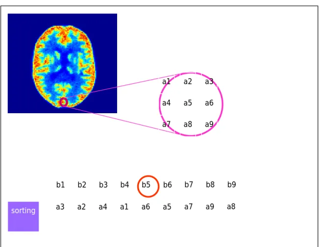
1. Partition the data into K clusters with similar sizes by sorting the means of xi in
T time frames and the initial centroids for K groups, {µ1, …, µK}, are calculated.
2. Let M = {M1 ,…,MN} denote the membership of N data points and Mi indicate
the cluster number for the data point xi as follows:
1 , min i i l k K i k M l if x µ x µ ≤ ≤ = − = − . 3. The centroids are updated by the memberships:
1 ( ) , N i k i i k x I M k n µ = =
∑
= × 0 ; ( ) 1 . i i i if M k I M k if M k ≠ ⎧ = = ⎨ = ⎩where nk represents the number of data points in the kth cluster.
4.
Repeat the second and third steps until the memberships M = {M1, …, MN}remain the same or the maximum number of iterations is achieved.
(2.2.1)
(2.2.3) (2.2.2)
2.3 Multivariate Normal Mixtures
For the study of dynamic images, the entire data is denoted by X = {x1, …, xN},
where xi represents the intensity vector for T time frames at one pixel of the image.
The Euclidean distance used in (2.2.1) for k-mean clustering is equivalent to assume that the distributions are normally distributed with normal distribution with different mean vectors and a common covariance matrix of σ2I, where σ2 is a variance scale and
I is an identity matrix. As the variance scale in every cluster may be different, we
can consider the model of multivariate normal mixture with different mean vectors and covariance matrices (McLachlan and Basford, 1988, Hsiao, Rangarajan, and Gindi, 1998).
Suppose that the probability that the data xi comes from the kth distribution is πk,
k K k k=1
0
1,
=1.
π
π
≤
≤
∑
Then the probability density function of xi becomes
(
)
(
)
1 , K , , i k k i k k f x π f x θ = Φ =∑
where fk(xi,θk) refers to the probability density function in the kth cluster with
parameters θk and the overall parameters are collected as
). ,..., , ,..., (π1 π K θ1 θK = Φ
Hence, we can write down likelihood function and log likelihood function for the observed incomplete data as follows:
(2.3.1)
(2.3.2)
( )
(
)
(
)
( )
(
)
(
)
1 1 1 1 1 1 ; , , log log ; log , . N in i i N K k k i k k i N in i i N K k k i k i k L f x f x L f x f x π θ π θ = = = = = = Φ = Φ ⎛ ⎞ = ⎜ ⎟ ⎝ ⎠ Φ = Φ ⎛ ⎞ = ⎜ ⎟ ⎝ ⎠∏
∑
∏
∏
∑
∑
Then, the maximum likelihood estimate (MLE) needs to solve the partial differential equations of
( )
log 0 in L ∂ Φ = ∂Φ .However, the above score functions are usually difficult to solve directly. The EM algorithm is applied to find the MLE iteratively (McLachlan and Basford, 1988, Hsiao, Rangarajan, and Gindi, 1998).
Firstly, we introduce the following index function:
1 if comes from kth normal distribution; 0 otherwise. i ik x Y ⎧ = ⎨ ⎩
and let Yi = (Yi1, …, YiK). These induces are not observed and {xi, Yi} form the
complete data for the EM algorithm. The conditional density of xi given Yi becomes
(
)
(
)
1 , K i i ik k i k k f x Y Y π f x θ = =∑
.The conditional log-likelihood turns out to be
( )
(
)
(
)
(
)
(
)
(
)
(
)
(
)
1 1 1 1 1 1 1 log log log , log , log log , . N i i i N K ik k i k i k N K ik k i k i k N K ik k i k i k L f x Y Y f x Y f x Y f x π θ π θ π θ = = = = = = = Φ = ⎛ ⎞ = ⎜ ⎟ ⎝ ⎠ = = +∏
∑
∑
∑∑
∑∑
The E-step calculates compute the conditional expectation of (2.3.11) given the initial parameter Φ(old) and X:
(2.3.4) (2.3.5) (2.3.6) (2.3.7) (2.3.8) (2.3.9) (2.3.10) (2.3.11) (2.3.12) (2.3.13) (2.3.14)
( )
(
; old)
(
log( )
, ( )old)
Q Φ Φ =E L Φ X Φ .
The M-step maximizes the above function with respect to Φ and the solution is used as Φ(new) to update the value of Φ(old).
For finite mixtures, we have
( )
(
)
(
( )
( ))
(
)
(
)
( ) ( )(
)
(
(
)
)
old old old 1 1 old 1 1 ; log , Y log log , , Y , log log , . N K ik k i k i k N K ik k i k i k Q E L X E f x x E x f x π θ π θ = = = = Φ Φ = Φ Φ ⎛ ⎞ = ⎜ + Φ ⎟ ⎝ ⎠ = Φ +∑∑
∑∑
So, we should evaluate E(Yik|x,Φ(old)) as follows:
( )
(
)
(
( ))
(
( ))
( )(
( ))
( )
(
( ))
old old old
old old old old 1 , 1 1 , 0 0 , , . , ik i ik i ik i k i k K k i k k E Y x f Y x f Y x f x f x π θ π θ = Φ = × = Φ + × = Φ =
∑
Hence, ( )(
)
( )( )(
( )( ))
(
)
(
(
)
)
old old k old old old 1 1 k ' ' 1 , ; log log , . , N K i k k i k K i k i k k f x Q f x f x π θ π θ π θ = = = Φ Φ =∑∑
+∑
Because of the constraint of πk in (2.3.2), we can use the Lagrange multiplier as
follows: ( )
(
old)
(
( )old)
1 ; ; ; K k 1 k Q λ Q λ π = ⎛ ⎞ Φ Φ = Φ Φ + ⎜ − ⎟ ⎝∑
⎠,where λ is in Lagrange multiplier parameter. By the constraint in (2.3.1) and (2.3.2), we have the solution for the local maximum in (2.3.21) and (2.3.22) for the normal mixture as follows: ( )
(
( ))
( )(
)
new old 1 old 1 1 , 1 , , N k i i N i i f k x f k x N π λ = = = − Φ = − Φ∑
∑
(2.3.15) (2.3.16) (2.3.17) (2.3.18) (2.3.19) (2.3.20) (2.3.21) (2.3.22) (2.3.23) (2.3.24)( ) ( )
(
)
( )(
)
old new 1 old 1 , , , N i i i k N i i f k x x f k x µ = = Φ = Φ∑
∑
( ) ( )(
)
(
( ))
(
( ))
( )(
)
old new new k k new 1 old 1 , , N T i i i i k N i i f k x x x f k x µ µ = = Φ − − Σ = Φ
∑
∑
, where(
)
(
)
( )
2 12(
)
1(
)
; ; , 1 2 exp . 2 k k k d T k k k k f x f x x x θ µ π − − µ − µ = Σ ⎛ ⎞ = Σ ⎜− − Σ − ⎟ ⎝ ⎠Thus, the EM algorithm for multivariate normal mixtures is described in the following algorithm.
Algorithm 2.3: The EM algorithm for multivariate normal mixtures 1. Set the initial parameters Φ(old).
2. Update the parameters by using (2.3.24), (2.3.25) and (2.3.26).
3. If log Lin (Φ(new) ) –log Lin (Φ(old) ) < tolerance, then the iteration stops.
Otherwise, go to Step 2 with the old values of parameters replaced by the new values.
2.4 Model Selection
How do we select the cluster size? Model selection criterion is useful to select the cluster size, like the Akaike information criterion (AIC) or Bayesian information criterion (BIC) (Akaike, 1969, Akaike, 1974, Rand, 1971). They are defined to balance the tradeoff between the maximum log-likelihood and the complexity penalty as follows:
(2.3.27) (2.3.25)
( )
2 log 2 , 2 log ln , AIC likelihood p BIC likelihood p N = − + ⎧ ⎨ = − + ⎩where p is the number of free parameters. It is shown that BIC is consistent and we will consider BIC. These two criteria are the same when the sample size is N =
7.389. When the sample size is greater than 7.389, the penalty term in BIC is bigger
than that in AIC. The sample size is 16384 * T in simulation and empirical studies of this report with the number of time frames in T. Hence, the BIC will select a simpler model with smaller clusters than the AIC will in these studies.
2.5 Tests for Homogeneity of Variances
If the variances are not the same, then we shall consider the normal mixtures instead of k-mean clustering. We can use tests of homogeneity of variances for this purpose. If the distributions in clusters are normally distributed, then the Bartlett test can be applied (Snedecor and Cochran, 1989). The hypotheses are
0 : i , 1, , ; 1 : a t le a s t o n e i .
H σ = σ i = K H σ ≠ σ
The following notations are defined:
1 ( ) , 0 ( ) . 1 N i k i i k i i i x I M k n if M k I M k if M k µ = = = × ≠ ⎧ = = ⎨ = ⎩
∑
(
)
2 2 1 ( ) , 1 N i k k i i k x S I M k n µ = − = = × −∑
(
)
(
)
2 2 1 1 1 . 1 K k k k K k k n S S n = = − = −∑
∑
(
)
2(
)
2 1 1 1 log 1 log , K K k k k k k D n S n S = = =∑
− −∑
− (2.5.1) (2.5.2) (2.5.3) (2.5.4) (2.4.1) (2.4.2)(
)
(
)
1 1 1 1 1 1 1 3 1 K K k k k k n n C K = = ⎛ ⎞ ⎜ ⎟ ⎜ − ⎟ − ⎜ − ⎟ ⎜ ⎟ ⎝ ⎠ = + −∑
∑
.UnderH , the quantity D C is approximately distributed as a0 2 1
K
x − variable. By a significance level α, we rejectH if 0 2
1,
K
D x
C> − α by the Bartlett test.
If the distributions in clusters are not normally distributed, then the Levene test can be applied (Levene, 1960). The Levene test is less sensitive the departure of normality than the Bartlett test is. Let
(
)
(
)
(
)
(
)
2 . .. 1 2 . .. 1 1 , 1 k K k k k n K k k j N K n Z Z W K Z Z = = = − − = − −∑
∑∑
whereZkj = xkj−xi. and x is the median of kth subgroup. Underi. H , the quantity 0 W is approximately distribution as anF(K−1,N K− ). By a significance level α, we rejectH if 0 W >F(K−1,N K− ,α) by the Levene test.
2.6 Dimension Reduction
In this study, the data amount is large and the computation costs in BIC become large. Dimension reduction methods can be applied to reduce the computation cost and suggest good initial cluster size. For example, the techniques of principal component analysis (PCA) (Hotelling, 1933) and regression in time can be applied. In PCA, we will select the leading principal components that explain more than 80% of variances. For regression in time, we use the regression slope in a linear regression model in time to reduce the dimension to one.
2.7 Cluster Merging in Segmentation
In microPET, there are a lot of factors that may cause noises in data. Multivariate normal mixtures are sensitive to noises and tend to separate noisy pixels into small clusters. K-mean clustering will have small clusters when the noise effect is large. Hence, we will merge neighboring clusters that have similar intensities. For example, we can test the distributions of mean intensities over time by the Kolmogorov-Smirno test (Feller, 1948).
2.8 Flow Charts
For comparison studies, three procedures are investigated in this report. The first procedure use the method of k-mean clustering and the second procedure uses the method of multivariate normal mixture. The third procedure uses tests of homogeneity for variances to select the clustering methods. If the homogeneity of variances is rejected, then the clustering results and the cluster size by k-mean clustering are used as the initial values in multivariate normal mixture of the original data. The flow charts are displayed below.
Procedure 1 and 2: 2 1 2 1 1 2 Dimension reduction by PCA or
Regression in time
Clustering the reduced data by k-mean
Clustering by the reduced data multivariate normal mixture
Find a cluster size K that minimizes BIC
Clustering the original data by k-mean
Clustering the original data by multivariate normal mixture Collect microPET data
Image reconstruction by MLEM
Cluster merging in segmentation
Expert evaluation 1
Procedure 3:
Dimension reduction by PCA or Regression in time
Clustering the reduced data by k-mean
Find a cluster size K that minimizes BIC
Clustering the original data by k-mean
Clustering the original data by multivariate normal mixture Collect microPET data
Image reconstruction by MLEM
Cluster merging in segmentation
Expert evaluation Tests of H0:
homogeneity for variances
0
accept H
0
Chapter 3. Simulation Studies
3.1 Simulation 1
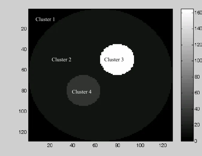
The phantom used in simulation 1 is displayed in Figure 1 of the Appendix. Those pixels outside the field-of-view (FOV) or region-of-interest (ROI) are put in Cluster 1. Inside the FOV or ROI, there are three clusters with different dynamic activities. Cluster 2 has similar activity as time increases. Cluster 3 has decreasing activity as time increases, whereas Cluster 4 has increasing activity as time increases. There are 128 by 128 pixels and 10 time frames simulated according to the model of (2.1.1) and (2.1.2) with D = 192 and *
( )
d d
λ / *
( )
p d
λ = 30%. Time-activity curves in Simulation 1 are plotted in Figure 2.
3.1.1 Procedure 1
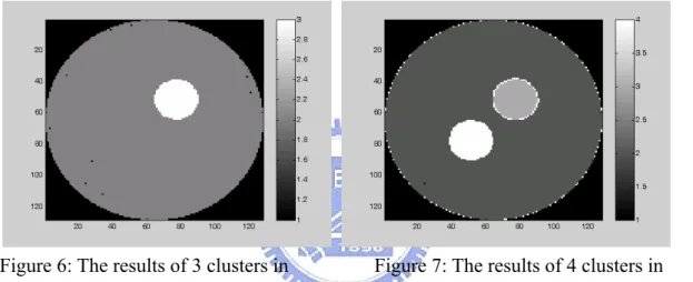
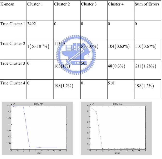
The PCA loadings of simulation 1 are plotted in Figure 3. The first principal component explains 86.9% of the variation and it is used for the purpose of dimension reduction. The BIC plots for k-mean clustering by PCA and regression in time are displayed in Figure 4 and 5 that both suggest the cluster size of 6. The segmentation results of k-mean clustering when the cluster size is 3, 4, 5, and 6 are shown in Figure 6, 7, 8, and 9. Hence, the selected cluster size of 6 results in small clusters caused by noise effects. The neighboring clusters with similar intensities can be merged from the cluster size of 6 to 4. However, the cluster size shall not be reduced from 4 to 3 since the neighboring clusters have different intensities.
The BIC plot of Simulation 1 for the original data by k-mean clustering is plotted in Figure 10. This BIC plot will select the correct cluster size this case. In any case, the cluster sizes selected by BIC with PCA or regression in time can provide a fast
approach to suggest a good initial size for searching the cluster size by BIC for the original data. Classification errors of k-mean clustering with cluster size 4 in Simulation 1 are reported in Table 1 of the Appendix.
3.1.2 Procedure 2
Similarly, we investigate the performance of normal mixture in Procedure 2 for Simulation 1. The BIC plots of normal mixture in Simulation 1 by PCA and regression in time are plotted in Figure 11 and 12, which suggest the cluster size of 6 and 5 that has the largest drops of BIC values respectively. The segmentation results of normal mixtures when the cluster size varies from 3 to 6 are displayed in Figure 13-16. These segmentation results of normal mixture in Figure 13-16 are similar in quality to those of k-mean clustering in Figure 6-9. The BIC plot of k-mean clustering in Simulation 1 for the original data by normal mixture clustering is plotted in Figure 17, which has the largest decrease of BIC value when the cluster size is 4. Classification errors of normal mixture with cluster size 4 in Simulation 1 are reported in Table 2, which are similar in quantity to those of k-mean clustering in Table 1. The error rate of normal mixture is better in Cluster 3 and 4, which have decreasing or increasing activities over time that are the major focus in dynamic studies.
3.1.3 Procedure 3
Procedure 3 is the combination of Procedure 2 and Procedure 1 with the test of homogeneity of variances. The results of Bartlett tests are reported in Table 3, which reject the null hypothesis in this case. Hence, Procedure 1 with normal mixture is used in this case.
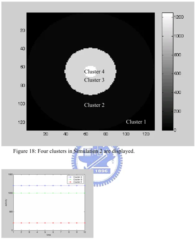
3.2 Simulation 2
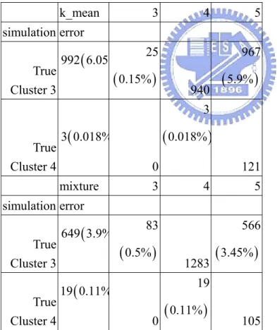
The phantom study in Simulation 2 is displayed in Figure 18, where there are nested clusters that are of interest. The segmentation results are reported in the Appendix. The error rate of normal mixture is better in Cluster 3 and 4 that have similar intensities. Because the simulations are based on the simulations of Poisson distributions in the model of (2.1.1) and (2.1.2), the variance is the same as the mean intensity for a Poisson distribution. So, Cluster 3 and 4 in these two simulations have high intensities and variances. Hence, clustering by normal mixture has higher accuracy to distinguishing the clusters with higher intensities over time in these two simulations.
Chapter 4. Empirical studies
The empirical data are collected from the mouse data from the MocroPET R4 system in Taiwan. There are 63 slices of the volume data and we use the middle
24th slice for investigation. There are 10 time frames. The MLEM reconstruction
of the first time frame is displayed in Figure 28. There are two clusters of regions with high intensities. We will proceed automatic clustering of this data by Procedure 3. The loading of principal components are shown in Figure 29. As the first principal component explains 85% of variation, it is selected as the dimension reduction method for PCA in this study. Linear regression in time is another method of dimension reduction in this study.
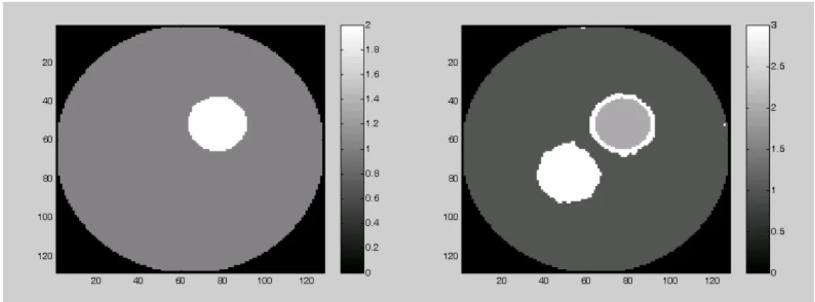
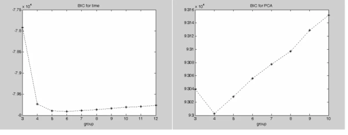
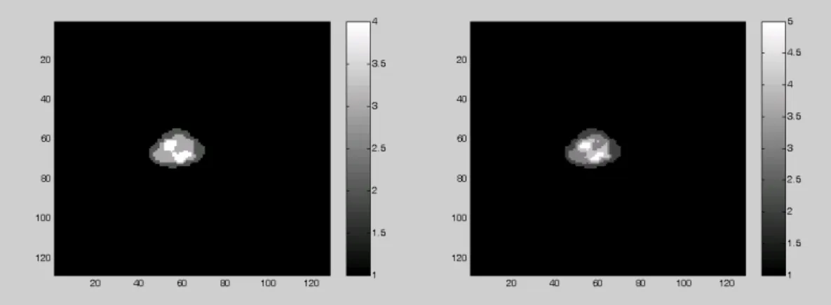
Firstly, k-mean clustering with dimension reduction methods is used to segment the dynamic images. The BIC plots of PCA and regression are displayed in Figure 31 and 30, which suggest that the cluster size can be 4 and 5. The segmentation results of 4 and 5 clusters for the original data by k-mean clustering are demonstrated in Figure 32 and 33.
The results of Bartlett tests are reported in Table 4, which reject the null hypothesis that the variances are equal in all clusters. Hence, the normal mixture is used to segment the images. The segmentation results by normal mixture are displayed in Figure 34-37. The qualities of segmentation results by k-mean clustering and normal mixtures are similar. The quantity differences can be evaluated by expertise in future studies.
Chapter 5. Conclusion and Discussion
We have proposed new methods to segment dynamic microPET images by MLEM reconstruction with k-mean or mixture clustering. The MLEM reconstruction is more precise than the FBP reconstruction with fewer artifacts. K-mean or mixture clustering can perform the segmentation automatically. Tests of homogeneity of variances are used to decide k-mean or mixture clustering. BIC is used to select the cluster size from the data adaptively. Dimension reduction techniques can be integrated to reduce the computation cost in determining the cluster size by BIC.
If the activities of various clusters have different temporary patterns, then regression in time is useful to distinguish them via dimension reduction. Otherwise, the principal component analysis is a general tool for dimension reduction. Besides simple linear regression, we can also consider polynomial or nonlinear regression in time.
Because the images of MLEM reconstruction may be still noisy, noise reduction filters can be applied to remove noises. For example, the median filter can be applied as demonstrated in Figure 38. Other filters that can remove noises and preserve edges are important for this purpose.
For further investigation of these methods, it will be of great interest to evaluate the quality and quantity performance by more phantom studies and empirical studies with the judgments from medical experts in the future.
References
1. Akaike H. Fitting autoregressive models for prediction. Ann. Inst. Stat. Math 1969; 21:243-247.
2. Akaike H. A new look at the statistical model identification. IEEE Trans.
Automat. Ontr., 1974, Dec.; vol. AC-19, pp. 716-723.
3. Chen JC, Tu KY, Lu HHS, Chen TB, Chou KL, Liu RS. Statistical Image Reconstruction for PET Studies. The Biomedical Engineering Society 1998
Annual Symposium. 1998; 71-72.
4. Chen JC, Liu R., Tu KY, Lu HHS, Chen TB, Chou KL. Iterative Image Reconstruction with Random Correction for PET studies. Proceedings of the
Society of Photo-Optical Instrumentation Engineers, 2000; 3979, 1218-1229.
5. Chen CM, Lu HHS, Hsu YP. Cross-Reference Maximum Likelihood Estimate Reconstruction for Positron Emission Tomography. Biomed. Eng. Appl. Basis
Comm., 2001; 13, 4, 190-198.
6. Cooper L. M-dimensional location models: Application to cluster analysis. J.
Reg. Sci., 1979; vol. 13, 99. 41-54.
7. Cunningham VJ, Jones T. Spectral analysis of dynamic PET studies. J. Cereb.
Blood Flow Metab., 1993; vol. 13, pp.15-23.
8. Dempster AP, Laird NM, Rubin DB. Maximum likelihood from incomplete data via the EM algorithm (with discussion). J. R. Statist. Soc. B, 1977; 39, 1-38. 9. Feller W. On the Kolmogorov-Smirno limit theorems for empirical distributions.
Ann. Math. Statist. 1948; 19 179-181.
10. Hotelling H. Analysis of a complex of statistical variables into principal components. Journal of Educational Psychology 1933; 24, 471-411, 498-520. 11. Hsiao IT, Rangarajan A, Gindi G. Joint-Map Reconstruction/Segmentation for
Science Symposium and Medical Image Conference, 1998; vol. 3, pp. 1689-1693.
12. Ollinger JM, Fessler JA. Positron-emission tomography. IEEE Signal Processing
Magazine, 1997 , January; Vol. 41, No.1, pp. 43-55.
13. Levene H. Robust tests for equality of variances. Contributions to Probability
and Statistics: Essays in Honor of Harold Hotelling, I. Olkin et al. eds. Stanford
University Press 1960; pp278-292.
14. Lu HHS, Chen CM, Yang IH. Cross-Reference Weighted Least Square Estimates for Positron Emission Tomography. IEEE Transactions on Medical Imaging, 1998; 17, 1, 1-8.
15. Lu HHS, Tseng WJ. On Accelerated Cross-Reference Maximum Likelihood Estimates for Positron Emission Tomography. Proceedings of the IEEE Nuclear
Science Symposium, 1997; Volume 2, 1484 -1488.
16. McLachlan G.J, Basford KE. Mixture Models: Inference and Applications to
Clustering. Dekker. 1988.
17. Politte DG., Snyder DL. Corrections for accidental coincidences and attenuation in maximum-likelihood image reconstruction for positron-emission tomography.
IEEE Transactions on Medical Image, 1991; vol. 10, no. 1, 99. 82-89.
18. Rand MW. Objective criteria for the Evaluation of clustering methods. Journal
of the American Statistical Association. 1971; 66, 846-850.
19. Snedecor GW, Cochran WG. Statistical Methods, Eighth Edition, Iowa State University Press. 1989.
20. Shepp LA, Vardi Y. Maximum likelihood reconstruction for emission tomography. IEEE Trans. Med. Image, 1982; vol. MI-1, 99. 113-122.
21. Tu KY, Chen JC, Lu HHS, Chen TB, Chou,KL, Liu RS. Iterative Image Reconstruction with Random Coincidence Correction for PET Studies. The
22. Tu KY, Chen JC, Lu HHS, Chen TB, Chou KL, Liu RS. Random Correction Using Iterative Reconstruction for PET. European Association of Nuclear
Medicine Annual Congress. 2000.
23. Tu KY, Chen, TB, Lu, HHS, Liu RS, Chen KL, Chen CM, Chen JC. Empirical Studies of Cross-Reference Maximum Likelihood Estimate Reconstruction for Positron Emission Tomography. Biomed. Eng. Appl. Basis Comm. 2001; 13, 1, 1-7.
24. Wong KP, Feng D, Meikle SR, Fulham MJ. Simultaneous estimation of physiological parameters and input function: In vivo PET data. IEEE Trans.
Inform. Technol. Biomed., 2001; vol. 5, pp. 67-76
25. Wong KP, Feng D, Meikle SR, Fulham MJ. Segmentation of Dynamic PET Images Using Cluster Analysis. IEEE Transactions on Nuclear Science, 2002, Feb.; vol. 49 no. 1.
26. Vardi Y, Shepp LA, Kaufman L. A statistical model for positron emission tomography. Journal of the American Statistical Association, 1985; vol. 80, no. 389, pp. 8-20.
27. Wu CFJ. On the convergence properties of the EM algorithm. Annals of Statistics, 1983; 11, 95-103.
Appendix
Figure 1: Four clusters in Simulation 1 within the size of 128 by 128 are displayed.
Figure 2: Time-activity curves in Simulation 1 are plotted.
Figure 3: PCA loadings of simulation 1 are plotted.
Cluster 4
Cluster 3
Cluster 2 Cluster 1
Figure 4: The BIC plot of k-mean clustering in Simulation 1 by PCA is displayed.
Figure 5: The BIC plot of k-mean clustering in Simulation 1 by regression is displayed.
Figure 6: The results of 3 clusters in
Simulation 1 by k-mean clustering are shown.
Figure 7: The results of 4 clusters in
Simulation 1 by k-mean clustering are shown.
Figure 8: The results of 5 clusters in
Simulation 1 by k-mean clustering are shown.
Figure 9: The results of 6 clusters in
K-mean Cluster 1 Cluster 2 Cluster 3 Cluster 4 Sum of Errors True Cluster 1 3492 0 0 0 0 True Cluster 2 1
(
6 10 %× −3)
11350 5(
0.03%)
104(
0.63%)
110 0.67%(
)
True Cluster 3 0 163( )
1% 505 48(
0.3%)
211 1.28%(
)
True Cluster 4 0 198(
1.2%)
0 518 198 1.2%(
)
Figure 10: The BIC plot of k-mean clustering in Simulation 1 for the original data by k-mean clustering is plotted.
Figure 11: The BIC plot of normal mixture in Simulation 1 by PCA is displayed.
Figure 12: The BIC plot of normal mixture in Simulation 1 by regression is displayed. Table 1: Classification errors and error rates of k-mean clustering in Simulation 1 are shown.
Figure 13: The results of 3 clusters in Simulation 1 by normal mixture are shown.
Figure 14: The results of 4 clusters in Simulation 1 by normal mixture are shown.
Figure 15: The results of 5 clusters in Simulation 1 by normal mixture are shown.
Figure 16: The results of 6 clusters in Simulation 1 by normal mixture are shown.
Figure 17: The BIC plot of normal mixture in Simulation 1 for the original data by normal mixture is plotted.
Normal mixture
Cluster 1 Cluster 2 Cluster 3 Cluster 4 Sum of Errors
True Cluster 1 3492 0 0 0 0 True Cluster 2 64
(
0.4%)
11211 12(
0.07%)
173(
1.05%)
249 1.52%(
)
True Cluster 3 0 85(
0.52%)
520 111(
0.68%)
196 1.2%(
)
True Cluster 4 0 112(
0.68%)
0 604 112 0.68%(
)
Table 2: Classification errors and error rates of normal mixture clustering in Simulation 1 are shown.
Figure 18: Four clusters in Simulation 2 are displayed. Cluster 4
Cluster 3
Cluster 2
Cluster 1
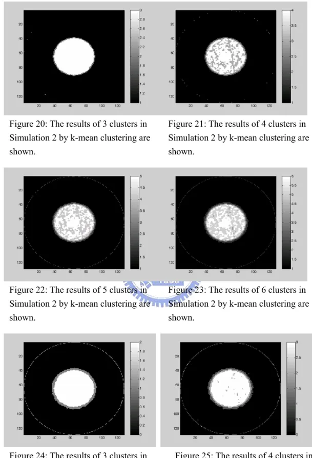
Figure 20: The results of 3 clusters in Simulation 2 by k-mean clustering are shown.
Figure 21: The results of 4 clusters in Simulation 2 by k-mean clustering are shown.
Figure 22: The results of 5 clusters in Simulation 2 by k-mean clustering are shown.
Figure 23: The results of 6 clusters in Simulation 2 by k-mean clustering are shown.
Figure 24: The results of 3 clusters in Simulation 2 by normal mixture are shown.
Figure 25: The results of 4 clusters in Simulation 2 by normal mixture are shown.
k_mean 3 4 5 simulation error True Cluster 3
(
992 6.05 25(
0.15%)
940 967(
5.9%)
True Cluster 4(
3 0.018% 0 3(
0.018%)
121 mixture 3 4 5 simulation error True Cluster 3(
649 3.9% 83(
0.5%)
1283 566(
3.45%)
True Cluster 4(
19 0.11% 0 19(
0.11%)
105 Figure 26: The results of 5 clusters inSimulation 2 by normal mixture are shown.
Figure 27: The results of 6 clusters in Simulation 2 by normal mixture are shown.
Table 3: Classification errors and error rates of k-mean and normal mixture clustering in Simulation 2 are shown.
Figure 28: Experiment data are displayed
Figure 29: PCA loadings of experiment data are plotted.
Figure 31: The BIC plot of k-mean Figure 30: The BIC plot of k-mean
groups P-Value Bartlett test 3 58141 0 Bartlett test 4 68401.68 0 Bartlett test 5 68969.65 0 Bartlett test 6 68180.45 0 Bartlett test 7 67808.42 0 Bartlett test 8 67689.87 0 Bartlett test 9 68524.84 0 Bartlett test 10 68193.19 0 Bartlett test 11 67974.98 0 Bartlett test 12 70109.08 0
Table 4: The results by the Bartlett test are reported. Figure 32: The results of 4 clusters in
experiment data by k-mean clustering are shown.
Figure 33: The results of 5 clusters in experiment data by k-mean clustering are shown.
Figure 34: The results of 3 clusters in experiment data by normal mixture are shown.
Figure 35: The results of 4 clusters in experiment data by normal mixture are shown.
a1 a4 a7 a2 a5 a8 a3 a6 a9 a1 a4 a2 a5 a3 a6 b4 b3 b8 b2 b6 b9 b1 b5 b7 a7 a9 a8 sorting
Figure 36: The results of 5 clusters in experiment data by normal mixture are shown.
Figure 37: The results of 6 clusters in experiment data by normal mixture are shown.
Figure 39: Time-activity curves of experiment data are plotted.