噴射式大氣電漿(APPJ)模擬研究---2D與3D平行化流體模型(II)

行政院國家科學委員會補助專題研究計畫完整報告

噴射式大氣電漿(APPJ)模擬研究-2D 與 3D 平行化流體模型(II)

Development and Applications of Parallelized 2D/3D Fluid Modeling Code

for Atmospheric-Pressure Plasma Jet

計畫類別：x 個別型計畫 □整合型計畫

計畫編號：97-NU-7-009-001-

執行期間：97 年 01 月 01 日至 97 年 12 月 31 日

計畫主持人：吳宗信

共同主持人：黃楓南 國立中央大學數學系

計畫參與人員：胡孟樺 國立交通大學機械工程學系

本成果報告包括以下應繳交之附件：

□ 赴國外出差或研習心得報告一份

□赴大陸地區出差或研習心得報告一份

□出席國際學術會議心得報告及發表之論文各一份

□國際合作研究計畫國外研究報告書一份

執行單位：國立交通大學機械工程學系

中 華 民 國

98 年 03 月 31 日

行政院國家科學委員會專題研究計畫期末報告

噴射式大氣電漿

(APPJ)模擬研究-2D 與 3D 平行化流體模型(II)

Development and Applications of Parallelized 2D/3D Fluid

Modeling Code for Atmospheric-Pressure Plasma Jet

計畫編號：97-NU-7-009-001-

執行期限：97 年 01 月 01 日至 97 年 12 月 31 日

主持人：吳宗信 國立交通大學機械工程學系

共同主持人：黃楓南 國立中央大學數學系

計畫參與人員：胡孟樺 國立交通大學機械工程學系

中文摘要 在此研究計畫裡，我們計劃使用流體模式的技 術，來模擬目前INER 所感興趣的噴射式大氣電漿 (APPJ)，或是更複雜的電漿狀態。因為帶電粒子 在鞘層區有很強的漂移效應(drift)，所以我們利用 FMD 將其連續方程離散化，而對於模擬各種流速 或流體所需的N-S equations，則FVM 離散之。所 有 離 散 之 耦 合 非 線 性 方 程 式 ， 將 利 用 Newton-Krylov-Schwarz (NKS)方法進行數值解析。而考慮 到APPJ 的幾何結構，在第一階段中我們首先發展 一套程式，用以模擬二維/軸對稱座標系統，之後 將程式延伸至三維座標系統，以處理更真實的操 作條件。所有的模擬程式將在PETSc 的DA 資料 結構下平行化。此後，程式可在任何平行化的機 器上執行，例如: PC clusters。總結來說，在這二 年的計劃裡，我們已完成平行化的NS equaton 及 fluidmodeling equation 的測試，詳細將在下列報 告中描述。 關鍵字: 噴射式大氣電漿, 漂移效應, 平行化 Abstract

In the proposed research project, we intend to apply the fluid modeling technique to simulate the atmospheric pressure plasma jet (APPJ), in which the INER is currently interested. Either finite-difference or finite-volume method was used to discrietize the governing equations. All discretized nonlinear equations will be solved using a Newton-Krylov-Schwarz (NKS) scheme. Considering the flat or

round APPJ, in which INER is interested, we will

first develop a simulation code for 2D/axisymmetric coordinate system in the first phase and then extend it into a 3D version in later phases to deal with more realistic operating conditions. All simulation codes will be parallelized under the DA framework of PETSC. Eventually, they shall be able to run on any

memory-distributed parallel machines, e.g., PC clusters. In summary, in the second year of the project we have completed the parallel implementation of NS equation and plasma fluid modeling equation. Results are presented and discussed in the report.

Keywords: APPJ, drift, parallel, fluid modeling, NS

equation

I. INTRODUCTION

Low-pressure plasmas have found wide applications in materials processing and others, and have contributed greatly in advancing the electronic semiconductor industry. The advantages of plasmas in materials processing include very efficient etching and film deposition. The temperature of the wafer can be kept low, which is important for electronics semiconductor processing. In addition, uniform glow discharge can be generated, which provides possibility of uniform processing for a very large surface.

However, operations at reduced pressure increase the cost dramatically since very expensive vacuum equipments have to be employed. Atmospheric-pressure plasmas overcome these inherited disadvantages of low-pressure plasmas and thus have attracted tremendous attention in the past 1-2 decades. On the other hand, several applications require the atmospheric or continuous in-line processing, which include surface modification, surface cleaning, sterilization/activation of bacteria cells, etching, and thin film deposition, among

others. However, research about APPs heavily relies on trial-and-error method, which is very time-consuming and unscientific in essence. Although there were several numerical studies available for APP in the literature, they often concentrated on one-dimensional simulation because of very high computational cost. However, more realistic numerical studies such as two-dimensional simulations are often required for understanding the plasma physics and thus help improving the design at the end. In addition, applications often require the use of post-discharge (jet) region of the APP, in which the fluid motion is very important in affecting the distribution of radicals that is the most critical issue terms of in application viewpoint. These leads to the strong motivation of developing efficient simulation technique for APPs.

II. NUMBERICAL METHOD [i] Neutral Flow Modeling a. Governing Equation

The current implementation attempts to solve both for the flow of charged particles (which are influenced by the presence of electric and magnetic fields) and the flow of an uncharged viscous carrier gas. The motion of the carrier gas, not influenced directly by the presence of electromagnetic fields, is given by the Navier-Stokes Equations in conservative form in two dimension:

[

v

] [

v

]

₀ U t x y F F G G ∂ ∂ ∂ ∂ ∂ ∂ − − + + =

(

)

(

)

0 0 0 xx xy xx xy x xy yy xy yy y t x y u uu u uv v u v q u E p E v vu vv u v q E p v ρ ρ τ ρ ρ τ ρ ρ τ τ ρ τ ρ τ ρ τ τ ∂ ∂ ∂ ∂ ∂ ∂ + − + + + + − + + + ⎧⎡ ⎤ ⎡ ⎤⎫ ⎡ ⎤ ⎪⎢ ⎥ ⎢ ⎥⎪ ⎢ ⎥ _{⎪ ⎪} ⎢ ⎥ ⎢ ⎥ ⎢ ⎥ _{⎨ ⎬} ⎢ ⎥ ⎢ ⎥ ⎢ ⎥ _{⎪ ⎪} ⎢ ⎥ ⎢ ⎥ ⎢ ⎥ _{⎪ ⎪} ⎣ ⎦ ⎩⎣ ⎦ ⎣ ⎦⎭ ⎧⎡ ⎤ ⎡ ⎤⎫ ⎪⎢ ⎥ ⎢ ⎥⎪ ⎪_{⎢ ⎥ ⎢ ⎥}⎪₌ ⎨_{⎢ ⎥ ⎢ ⎥}⎬ ⎪_{⎢ ⎥ ⎢ ⎥}⎪ ⎪_{⎣ ⎦} ⎪ ⎩ ⎣ ⎦⎭

where µ and η are the first and second coefficients of viscosity respectively (related by Stoke’s Hypothesis), ρ is the carrier gas

density, u and v the carrier gas x and y components of velocities, E the total energy of the gas (per unit mass) and p the gas pressure.

b. Numerical Algorithm

Spatial Discretization

The cell-centered scheme is employed here then the control volume surface can be represented by the cell surfaces and the coding structure can be much simplified. The transport equations can also be written in integral form as:

d F nd S d

t_Ωρφ _{Γ Ω} Ω

∂

Ω + ⋅ Γ = Ω

∂

∫

∫

∫

where Ω is the domain of interest, Γ the surrounding surface, n the unit normal in outward direction. The flux function F consists of the inviscid and the viscous parts:

φ µ φ ρ − _φ∇ = V F

The finite volume formulation of flux integral can be evaluated by the summation of the flux vectors over each face,

( ) i j, j j k i F nd F = Γ ⋅ Γ =

∑

∆Γ

∫

where k(i) is a list of faces of cell i, Fi,j represents convection and diffusion fluxes through the interface between cell i and j,

j

∆Γ is the cell-face area.

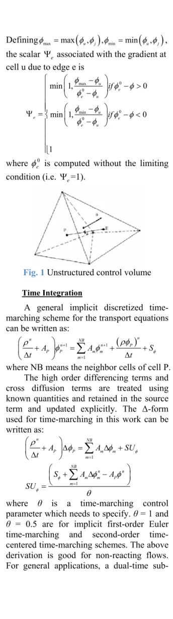
The viscous flux for the face e between control volumes P and E as shown in Fig. 1

can be approximated as:

(

)

E P E P e e E P E r r n n r r r r φ φ φ − φ − ∇ ⋅ ≈ + ∇ ⋅ − − − ⎛ ⎞ ⎜ ⎟ ⎝ ⎠

That is based on the consideration that

(

)

E P e rE rP

φ −φ ≈ ∇ ⋅φ −

where ∇ is interpolated from the neighbor φ cells E and P.

The inviscid flux is evaluated through the values at the upwind cell and a linear reconstruction procedure to achieve second order accuracy

φ_e =φ_u +Ψ_e∇φ_u⋅

(

r_e−r_u

)

where the subscript u represents the upwind cell and Ψ is a flux limiter used to prevent _e from local extreme introduced by the data reconstruction. The flux limiter proposed by Barth [21] is employed in this work.

Definingφ_max =max

(

φ φ φ_u, _j

)

, _min =min

(

φ φ_u, _j

)

, the scalar Ψ associated with the gradient at _e cell u due to edge e is

0 max 0 0 min 0 min 1, 0 min 1, 0 1 u e e u u e e e u if if φ φ _{φ φ} φ φ φ φ _{φ φ} φ φ − − > − − Ψ = − < − ⎧ ⎛ ⎞ ⎜ ⎟ ⎪ ⎝ ⎠ ⎪ ⎪⎪ ⎛ ⎞ ⎨ _{⎜ ⎟} ⎝ ⎠ ⎪ ⎪ ⎪ ⎪⎩ where 0 e

φ is computed without the limiting condition (i.e. Ψ =1). _e

Fig. 1 Unstructured control volume

Time Integration

A general implicit discretized time-marching scheme for the transport equations can be written as:

(

)

1 1 1 n n NB n n P P P m m m A A S t t φ ρφ ρ _φ + _φ + = + = + + ∆ ∆ ⎛ ⎞ ⎜ ⎟ ⎝ ⎠

∑

where NB means the neighbor cells of cell P. The high order differencing terms and cross diffusion terms are treated using known quantities and retained in the source term and updated explicitly. The ∆-form used for time-marching in this work can be written as: 1 n NB P P m m m A A SU t φ ρ _{φ φ} = + ∆ = ∆ + ∆ ⎛ ⎞ ⎜ ⎟ ⎝ ⎠

∑

1 NB n n m m P m S A A SU φ φ φ φ θ = + ∆ − = ⎛ ⎞ ⎜ ⎟ ⎝

∑

⎠

where θ is a time-marching control parameter which needs to specify. θ = 1 and θ = 0.5 are for implicit first-order Euler marching and second-order time-centered time-marching schemes. The above derivation is good for non-reacting flows. For general applications, a dual-time

sub-iteration method is now used in UNIC-UNS for time-accurate time-marching computations.

Pressure-Velocity-Density Coupling

In an extended SIMPLE [14] family pressure-correction algorithm, the pressure correction equation for all-speed flow is formulated using the perturbed equation of state, momentum and continuity equations.

The simplified formulation can be written as: 1 1 ; ; n n ; n n u u D p u u u p p p RT ρ ρ γ + + ′ ′= ′= − ∇ ′ = + ′ = + ′

( )

( )

( )

n n u u u t t ρ′ _{ρ ρ} ρ _ρ ∂ _{′ ′} ∂ + ∇ + ∇ = − − ∇ ∂ ∂ ⎛ ⎞ ⎜ ⎟ ⎝ ⎠

where Du is the pressure-velocity coupling coefficient. The following all-speed pressure-correction equation is obtained,

(

)

( )

1 n n u p D p u RT t t ρ ρ ρ γ ′ _∆ ′ ′ ⋅ + ∇ ⋅ ∇ = − − ∇ ⋅ ∆ ∆ ⎛ ⎞ ⎜ ⎟ ⎝ ⎠

For the cell-centered scheme, the flux integration is conducted along each face and its contribution is sent to the two cells on either side of the interface. Once the integration loop is performed along the face index, the discretization of the governing equations is completed. First, the momentum equation is solved implicitly at the predictor step. Once the solution of pressure-correction equation is obtained, the velocity, pressure and density fields are updated. The entire corrector step is repeated 2 and 3 times so that the mass conservation is enforced. The scalar equations such as turbulence transport equations, species equations etc. are then solved sequentially. Then, the solution procedure marches to the next time level for transient calculations or global iteration for steady-state calculations. Unlike for incompressible flow, the pressure-correction equation, which contains both convective and diffusive terms are essentially transport-like.

High Order Schemes

The challenge in constructing an effective higher-order scheme is to determine an accurate estimate of flux at the

cell faces. Barth and Jespersen [22] proposed a multi-dimensional linear reconstruction approach, which forms the basis for the present scheme. In the cell reconstruction approach, higher-order accuracy is achieved by expanding the cell-centered solution to each cell face with a Taylor series:

(

_{, ,}

)

(

_{, ,}

)

( )

2

c c c c

q x y z =q x y z + ∇ ⋅ ∆ +q r O ∆r where q=

[

ρ, , , , ,u v w t dk de,

]

T

This formulation requires that the solution gradient be known at the cell centers. Here a scheme proposed in [18] is employed to compute the gradients:

qd qnd

Ω Γ

∇ Ω = Γ

∫

∫

The general approach was to: 1) coalesce surrounding cell information to the vertices or nodes of the candidate cell, then 2) apply the midpoint-trapezoidal rule to evaluate the surface integral of the gradient theorem 1 q qnd Γ ∇ = Γ Ω

∫

over the faces of each cells. Here Ω denotes the volume enclosed by the surface Γ.

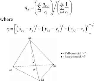
It is possible to further simplify the method for triangle (2D) or tetrahedron (3D) cells such that need not be evaluated explicitly. The simplification stems from the useful geometrical invariant features of triangle and tetrahedron. These features are illustrated for an arbitrary tetrahedral cell in

Fig. 2 Note that a line extending from a

cell-vertex through the cell-centroid will always intersect the centroid of the opposing face. Furthermore, the distance from the cell-vertex to the cell centroid is always three fourths of that from the vertex to the opposing face (For a triangle, the comparable ration of distance is two-thirds). By using these invariants along with the fact that Δr is the distance between them, the above equation can be evaluated as:

(

1 2 3

)

4 1 3 4 n n n n c q q q q q q r r r r r + + − ∂ ∇ ⋅ ∆ = ∆ ≈ ∆ ∂ ∆

Thus q(x,y,z) can be approximated for tetrahedral cells by the simple formula:

(

)

1,2,3 1 2 3 4 1 3 1 4 f c n n n n q =q + ⎡_⎣ q +q +q −q ⎤_⎦ where as illustrated in Fig. 2, the subscripts n1, n2 and n3 denote the nodes comprising face f1,2,3 of cell c and n4 corresponds to the opposite node. This modified scheme is analytically equivalent to that in [18] and results in a factor of two reductions in computational time of the flow solver.

The nodal quantities qn are determined in the manner described in [18]. Accordingly, estimates of the solution are determined at each node by a weighted average of the surrounding cell-centered solution quantities. It is assumed in the nodal averaging procedure that the known values of the solution are concentrated at the cell centers, and that the contribution to a node from the surrounding cells is inversely proportional to the distance from each cell centroid to the node:

, 1 ₁ 1 i N _{c i} N n i i i q q r r = ₌ ⎛ ⎞ ⎛ ⎞ = ∑_{⎜ ⎟ ⎜}∑ _⎟ ⎝ ⎠ ⎝ ⎠ where

(

) (

₂

) (

₂

)

₂ 1 2 , , , i c i n c i n c i n r =_⎣⎡ x −x + y −y + z −z ⎤_⎦

Fig. 2 Reconstruction stencil for tetrahedral cell-centered scheme

Until recently, the sole approach for the reconstruction was a pseudo-Laplacian averaging scheme presented in [17]. This scheme offers the advantage of second-order accuracy in reconstructing data from surrounding cells to a node. However, there is a need to artificially ‘clip’ the weighting factors between 0 and 2 [6] to avert a violation of the positivity principle, which is necessary for solution stability. This artificial ‘clipping’ process does, unfortunately, compromise the formal second-order accuracy of the scheme to some extent. Recent experience of applying

the pseudo-Lapacian scheme to Navier-Stokes computations has surfaced some anomalous behavior, which needs further investigation. Meanwhile, for the present work, we are temporarily reverting to the inverse-distance averaging of qn, which represents only acceptable accuracy, but will never violate the principle of positivity.

Pressure Damping

Following the concept of Rhie and Chow [4] developed for structured grid method to avoid the even-odd decoupling of velocity and pressure fields, a pressure damping term can also introduced for unstructured grid method when evaluating the interface mass flux. This form is written as: p p r r E p E p U U Du_e p_e e e _{r r} r r E p _{E p} − − = − ⋅ − ∇ ⋅ − ₋ ⎛ ⎞ ⎜ ⎟ ⎜ ⎟ ⎜ ⎟ ⎝ ⎠

whereU , _e ∇p_e and Due are interpolated

from the neighboring cells E and P, respectively. The last term on the right hand side is a higher order pressure damping term projected in the direction PE .

Boundary Conditions

Several different types of boundaries may be encountered in flow calculations, such as inflow, outflow, impermeable wall and symmetry. In the case of viscous incompressible flows, the following boundary conditions usually apply:

¾ The velocities and temperature are prescribed at the inlet;

¾ Zero normal gradient for the parallel velocity component and for all scalar quantities, and zero normal velocity component are specified at symmetry planes or axes;

¾ No-slip condition and prescribed temperature or heat flux are specified at the walls;

¾ Zero (or constant non-zero) gradient of all variables is specified at the outlet.

In the case of compressible flows, some new boundary conditions may apply:

¾ Prescribed total conditions (pressure, temperature) and flow direction at inflow;

¾ Prescribed static pressure at outflow; ¾ Supersonic outflow.

Some of these boundary conditions are straightforward to implement the detailed implementation is described in [32].

In order to facilitate the variations of inlet operating conditions in rocket engine applications, an inlet data mapping tool is developed. This inlet data-mapping tool accepts multiple patches of surface data. Each individual surface data patch is a structured grid that contains flow field data such as velocity, pressure, temperature, turbulence quantities and species concentrations, etc.

At start up, the UNIC code reads input data file and restart flow field data, then it will check the existence of the inlet boundary condition file, bcdata.dat. If inlet data is obtained from the inlet boundary condition file, data mapping procedure is then performed to incorporate the new inlet conditions.

Linear Matrix Solver

The discretized finite-volume equations can be represented by a set of linear algebra equations, which are non-symmetric matrix system with arbitrary scarcity patterns. Due to the diagonal dominant for the matrixes of the transport equations, they can converge even through the classical iterative methods. However, the coefficient matrix for the pressure-correction equation may be ill conditioned and the classical iterative methods may break down or converge slowly. Because satisfaction of the continuity equation is of crucial importance to guarantee the overall convergence, most of the computing time in fluid flow calculation is spent on solving the pressure-correction equation by which the continuity-satisfying flow field is enforced. Therefore the preconditioned Bi-CGSTAB [15] and GMRES [20] matrix solvers are used to efficiently solve, respectively, transports equation and pressure-correction equation.

Compared with a structured grid approach, the unstructured grid algorithm is more memory and CPU intensive because “links” between nodes, faces, cells, needs to be established explicitly, and many efficient solution methods developed for structured grids such as approximate factorization, line relaxation, SIS, etc. cannot be used for unstructured methods.

As a result, numerical simulation of three-dimensional flow fields remains very expensive even with today’s high-speed computers. As it is becoming more and more difficult to increase the speed and storage of conventional supercomputers, a parallel architecture wherein many processors are put together to work on the same problem seems to be the only alternative. In theory, the power of parallel computing is unlimited. It is reasonable to claim that parallel computing can provide the ultimate throughput for large-scale scientific and engineering applications. It has been demonstrated that performance that rivals or even surpasses supercomputers can be achieved on parallel computers. c. Flowchart

Fig. 3 Flowchart of the Navier-Stokes Modeling

[ii] Fluid Modeling a. Governing Equation

The continuity equation for ionized species and electrons are:

1 1 , 1, , p i e i p e r p p i r e e i n t n t S p k S = = ∂ ∂ ∂ ∂ + ∇ ⋅ Γ = = + ∇ ⋅ Γ =

∑

∑

…

where np and ne are the number density of

ion species p and electrons e respectively, k

is the number of ion species, rp is the

number of reaction channels that involve the creation and destroy of ion species p, and Γ is the particle flux. The electric field E is calculated from the potential field ψ which is in turn calculated from Poisson’s equation:

2 1 1 k i i e i q n en ψ ε− = ∇ = ⎛_⎜ − ⎞_⎟ ⎝

∑

⎠ and E= −∇ψ

where ε is the permittivity and can vary depending on the material (and therefore location in the simulation). The source terms in each of the charged particle continuity equations depends highly on the electron energy density which is governed by the equation:

(

)

1 c 3 e S i e i i e B m e g n t e E m S n k v T T M ε ε ε = ∂ ∂ + ∇ ⋅ Γ = − Γ ⋅ −

∑

+ −

(

)

5 5 2 2 ne e e B e B e B e e m n k T k T k T m v Γ = Γ − ∇

where nε (=3/2nekBTe) is the electron energy

density, Te is the electron temperature, εi is

the energy loss for the ith inelastic electron collision, kb is Boltzmann’s constant, νm is

the momentum exchange collision frequency between electron (mass me) and background

neutral (mass M), and Tg is the background

gas temperature.

b. Numerical Algorithm

Scharfetter-Gummel Scheme

The Scharfetter-Gummel Scheme provides an optimum way to descretize the drift-diffusion equation for particle transport. For an one-dimensional example, here defines the grid points i and i + 1, and the flux between the grids Γi+1/2. The

drift-diffusion equation of positive charged particle can be written as

1 1 1 , , , 2 2 2 p p p i p i p i n D n x x φ µ + + + ∂ ∂ Γ = − − ∂ ∂

The drift velocity ₁ , 2 p i x φ µ + ∂ ∂ is correlated to the density np through the self-consistent description of fluid modeling. We can

change the valuable from position to potential by chain rule,

1 1 , , 2 2 1 1 , , 2 2 p i p i p p p i p i n n x D x D µ φ φ φ + + + + Γ ∂ ∂ ∂ + = − ∂ ∂ ∂

, which here assume that the x φ ∂ ∂ is independent of potential, 1 1 , , 2 2 1 , 1 2 , 2 p i p i p p p i p i n n D _D x µ φ φ + + + + Γ ∂ + = − ∂ ∂ ∂

The solution of the first-order different equation is

( )

1 , 2 1 , 2 1 , 2 1 , 2 p i p i D _{p i} p p i n Ce D x µ φ φ _φ + + − + + Γ = − ∂ ∂

By applying the boundary condition

( )

i i i

n =n φ and n_i+1=n_i+1

( )

φ_i+1 , the constant C and flux Γ_{p i, 1/ 2+} can be found,

1 1 , , 2 2 1 1 1 , , 2 2 1 p i p i i i p i p i i i D D n n C e e µ µ φ φ + + + + + + − − − = −

( )

( )

[

]

1 , 2 1 1 , 2 p i i i p i D n B X n B X x + + + Γ = − − − ∆ , where , 1/ 2

(

)

1 , 1/ 2 p i i i p i X D µ φ φ + + + = − , and B is Bernoulli function,

( )

1 x X B x e = −

For electron, in the same way we can write the flux equation,

(

)

(

)

1 _e e e B e e e e B e e B e e e e e qn n k T E m v m v n k T qn k T n E m v m v m v Γ = − ∇ − = − ∇ − ∇ −

The first-order differential equation and its solution are

(

B e

)

B e e e e e e e k T k T q n E n m v m v m v ∇ ∇ +⎛_⎜ + ⎞_⎟ = −Γ ⎝ ⎠

(

B e

)

e e e B e B e B e e k T q n E n k T k T k T m v ∇ Γ ∇ +⎛_⎜ + ⎞_⎟ = − ⎝ ⎠

We can change the variable from position to potential and find the solution of density in function of potential.

( )

a x e b n Ce a φ φ φ −_∂ ∂ = +

, where C is a constant, as well as a and b are defined as

(

B e

)

B e B e k T q a E k T k T ∇ = + e B e e b k T m v Γ = −

For a given boundary at i+1 and i, we can know the constant C and the flux Γ , _e

1 1 i i i i a a n n C e φ+ e φ + ′ ′ − − − = −

( )

( )

, 1/ 2 1 1 _{B e} e i i i e k T B X n B X n x m v + + Γ = − ⎡_⎣ − − ⎤_⎦ ∆ , where X =a′

(

φ_i+1−φ_i

)

and a a x φ ′ = _∂ ∂

( )

( )

, 1/ 2 , 1/ 2 1 e i e i i i D n B X n B X x + + + Γ = − ⎡_⎣ − − ⎤_⎦ ∆ Nondimensionization

Here let n0 denote the background gas

density, and potential, length, time, and velocity scaling are list as following:

0 0 B e k T φ φ φ φ ′ = = , 0 p p u u u ′ = , 0 e e u u u ′ = , where u₀ is 1/ 2 0 0 B p k T u m ⎛ ⎞ = ⎜_⎜ ⎟_⎟ ⎝ ⎠

The normalized energy density is

,0 0 B 0 n n n k T ε ε = , and the normalized energy

0

B

e k T

ε′ = ε

, which the ε is in unit eV. x x

λ

′ = , where the character length is

0 1 p n λ σ =

, and the cross-section of Argon ion is

19 2

8.0 10

Ar m

σ +

−

= × . The character time scale is 0 u t t λ ′ =

The dimensionless diffusivity and permittivity are 0 D D u λ ′ = , m up 0 e µ µ λ ′ =

The ion momentum with drift-diffusion approximation and S-G scheme can be scaled

( )

( )

[

]

0 , 1/ 2 , 1/ 2 0 1 0 p i p i i i u D n n B X n n B X x λ λ + + + ′ ′ ′ Γ = − − − ′ ∆

( )

( )

[

]

, 1/ 2 , 1/ 2 1 p i p i i i D n B X n B X x + + + ′ ′ ′ ′ Γ = − − − ′ ∆ , also electron flux

( )

( )

[

]

, 1/ 2 , 1/ 2 1 e i e i i i D n B X n B X x + + + ′ ′ ′ ′ Γ = − − − ′ ∆

The scaling of continuity equation can be written as , 0 0 0 0 0 0 , , 1 e p e p e p n n u n u n u S t λ λ λ ′ ∂ ′ ′ ′ + ∇ ⋅ Γ = ′ ∂ , , , e p e p e p n S t ′ ∂ ′ ′ ′ + ∇ ⋅Γ = ′ ∂

The energy equation

0 0 0 0 0 0 0 0 0 1 B B B u n u n k T n k T u n k T S t ε ε ε λ λ λ ′ ∂ _{′ ′ ′} + ∇ ⋅ Γ = ′ ∂ n S t ε ε ε ′ ∂ _{′ ′ ′} + ∇ ⋅Γ = ′ ∂

, where the normalized energy source term is

e e S S E e ε ε′ ′ = − ′− Γ The scaling of Poisson’s equation,

2 0 0 2 0 1 B 1 s s s k T q n n e φ λ ∇′ ′= −ε

∑

(

)

2 2 2 0 0 s s B e e n sign n k T λ φ ε ′ ′ ′ ∇ = −

∑

(

)

2 1 s s sign n φ ε ′ ′ ′ ∇ = − ′

∑

, where 2 0 2 2 0 o p u m e n ε ε λ ′ =

Finite Difference Descritization

In this report, we descritize the fluid modeling equations through the use of finite difference method. Since continuity equations for different species are similar, here only presents the discretization for the equation. By employing the backward Euler scheme for time integration and the Sharfetter-Gummel scheme for representing the particle flux and after tedious algebraic rearrangement, the resulting discretized equation on a typical grid point (m, n) can be written as, , , , , , , , 1/ 2, , 1/ 2, , , 1/ 2 , , 1/ 2 , , 1 t t t m n m n t t m n m t t t t t t t t m n m n m n m n t t m n i m n n n t x S x y α α α α α α α α α γ +∆ +∆ +∆ +∆ +∆ +∆ + − + − +∆ = − + Γ ∆ Γ − Γ Γ − Γ + + = ∆ ∆

∑

, where α can be electrons, ion, and uncharged species, xm is the distance from original point to grid point m, ∆ and x_m ∆ y_m are the step length at grid (m, n), γ is a factor using to deal with the coordinate system, for cylindrical coordinate is 1 and for Cartesian coordinate is 0, Γ are the flux defined _α between grids which can be expressed in Scharfetter-Gummel form as,

( )

(

)

( )

(

)

1/ 2 , 1/ 2 1/ 2 , 1 1/ 2 , 1/ 2 m m m m m m m D x n B sign q X n B sign q X α α α α α + + + + + + Γ = − ∆ ⎡ − ⎣ ⎤ − − _⎦

( )

(

)

( )

(

)

1/ 2 , 1/ 2 1/ 2 , 1 1/ 2 , 1/ 2 n n n n n n n D x n B sign q X n B sign q X α α α α α + + + + + + Γ = − ∆ ⎡ − ⎣ ⎤ − − _⎦

, where X is a non-dimensional variable define as,

(

)

(

)

1/ 2 1/ 2 1 1/ 2 1/ 2 1/ 2 1 1/ 2 m m m m m n n n n n X D X D µ φ φ µ φ φ + + + + + + + + = − = −

, and B is the Bernoulli function which is defined as,

( )

1 x x B x e = −

The electron energy equation is descritized as

(

)

, , , , , , , , , , , 1/ 2, , 1/ 2, , , 1/ 2 , , 1/ 2 , , , , , , , 1 3 2 3 i t t t t t t e m n e m n e m n e m n t t e m n m t t t t t t t t e m n e m n e m n e m n m n S t t t t t t e t t e m n m n i m n e B m e m n g i n T n T t x x y m E S n k v T T M ε ε γ ε +∆ +∆ +∆ +∆ +∆ +∆ +∆ + − + − +∆ +∆ +∆ +∆ = − + Γ ∆ Γ − Γ Γ − Γ + + ∆ ∆ = −Γ ⋅ −

∑

− −

, where Te and ε_i are in unit of eV, ν_m is the electron collision frequency, and the descretized form energy fluxes Γ are ε expressed as, , , , 1/ 2, , 1, , 1/ 2, , 1/ 2, , 1/ 2, , 1/ 2, 5 5 2 2 e m n m n e m n e m n e m n e m n e m n e m m T T n T T m v x ε + + + + + + Γ = − Γ − ∆ , , , , 1/ 2 , , 1 , , 1/ 2 , , 1/ 2 , , 1/ 2 , , 1/ 2 5 5 2 2 e m n m n e m n e m n e m n e m n e m n e m n T T n T T m v y ε + + + + + + Γ = − Γ − ∆ Finally, the Poisson’s equation is discretized as

(

)

(

)

(

)

(

)

(

)

(

)

(

)

1 1/ 2 1 1/ 2 1 2 1/ 2 1 1/ 2 1 2 2 1 1 t t t t m m m m m t t t t t t t t m m m m m m m t t t t t t t t n n n n n n n x x x y γε _{φ φ} ε φ φ ε φ φ ε φ φ ε φ φ +∆ +∆ + +∆ +∆ +∆ +∆ + + − − +∆ +∆ +∆ +∆ + + − − − ∆ + − − − ∆ + − − − ∆

Parallel Newton-Krylov-Swartz Algorithm

In this study, the parallel fully coupled Newton-Krylov-Swartz(NKS) algorithm [11] to solve the large sparse system of nonlinear discretized equations, which are derived in the previous section, has applied. All the functions for each dependent variables are form a global functional vector. Jacobian matrix is then computed based on this global vector. Nevertheless, this treatment results in a fully implicit scheme, which allows much larger time step as compared to semi-implicit or explicit scheme. Another advantage of solving the coupled equations directly, rather than solving the equations one by one or some heuristic way of

coupling, is that it can have better time accuracy with appreciable time-step size, and much better parallel performance since the grain size is much larger. In this method, an inexact Newton method is used to solve the coupled nonlinear discretized equations at each time step. The resulting Jacobian system computed by using finite difference for the Newton corrections are solved with a preconditioned Krylov subspace type method, relying directly only on iterative operations. The Krylov method requires preconditioning for achieving acceptable convergence speed of inner interactions. A good preconditioner saves time and memory by allowing fewer iterations in the Krylov loop and smaller storage for the Krylov subspace. In this study, we have utilized a parallel additive Schwarz(AZ) type preconditioner with an inexact or exact solver such as incomplete LU(ILU) or LU factorizations in each subdomain. It was shown that this AS preconditioner can greatly reduce the runtime required for inner iterations in an inexact Newton method [3]. This results from that the smaller subdomain blocks maintain better cache residency and shorter convergence time for an approximate solver. In addition, either scheme was used to solve the preconditioned matrix equation at each time step. By combining the AS preconditioner with Krylov type subspace method BiCG-STAB(or BCGS) [12] or GMRES [19] in the present study within an inexact Newton method leads to a coherent fully parallel solver: Newton-Krylov-Schwarz(NKS) algorithm [16].

In practical implementation, we employed the PETSc package [9], which features distributed data structure –index sets, vectors, and matrices – as functional objects. Iterative linear and nonlinear solvers are combined modularly, recursively, and extensively through a uniform application programmer interface. In addition, the Jacobian system within the inexact Newton method can be computed automatically by the finite-difference scheme within the PETSc framework or by the user himself/herself. Portability is achieved through MPI, which is a stander in message passing among processors nowadays,

although the details are not requires in practical coding. All the codes were programmed in C/C++.

III. RESULTS AND DISCUSSIONS [i] Neutral Flow Modeling

The driven flow in a square cavity is used as the model problem. Solutions are obtained for configurations with meshes consisting of as many as 129 x 129 points.

The streamline contours for the cavity flow configurations with Re increasing from 100 to 5000 are shown in Fig. 4. As is well known, the center of primary vortex is offset toward s the top right corner at Re =100. It moves towards the geometric center of the cavity with increasing Re.

Compare these results with Ghia(1982, Fig 5. left), we can verify our Navier-Stokes Model is valid.

Fig. 4a Streamline pattern of Re=100

Fig. 4b Streamline pattern of Re=400

Fig. 4c Streamline pattern of Re=1000

Fig. 4d Streamline pattern of Re=3200

Fig. 4e Streamline pattern of Re=5000

[ii] Fluid Modeling

The results shown in the following are adapted from the simulation of an argon gas flowing through two parallel electrode with gap distance of 1 mm and length of 50 mm (Fig. 5), in which the discharged is maintained by a RF power source (f=13.56 MHz) with amplitude of 300 Volt. The simulation domain includes the post-discharge (jet) region, which is important in APPJ applications. The potential field, predicted electron and ion number density and general flow features are in general agreement between the two solvers.

Fig. 5 Details of the simulation performed

by the FDM (top) and FVM (bottom) showing the distant target body (lower).

In addition, simulation conditions included: 6 unknowns (Φ, Te, ne, nAr, nAr+, nmetastable, nresonance) in each grid point, 100 time steps in each RF cycle, 10-4 of relative convergence for the Newton iteration, 10-5 of relative convergence for the KSP matrix solver. Mobility and diffusivity of argon ions was taken to be 0.14 m2V-1s-1 and 4*10 -3 _m2_s-1_{, respectively [13]. In parallel}

computing, an ASM preconditioner using only one overlapping layer with LU as the subdomain solver was employed. A relatively simple plasma chemistry was considered as summarized in Table 1.

Table 1. Argon plasma chemistry.

a. Parallel Performance Testing

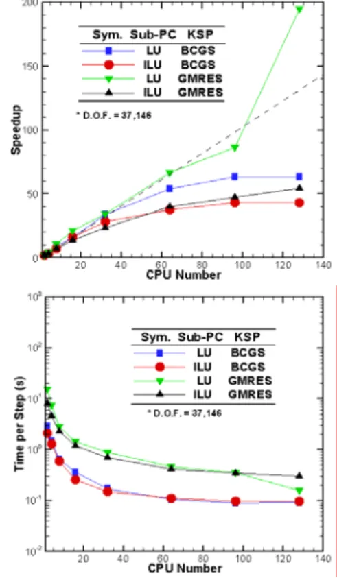
Fig. 6 illustrates the parallel

performance related results as a function of the number of processors. Fig. 6a shows that the parallel speedup for the cases using GMRES as the KSP solve and LU as the subdomain solver in the preconditioner generally perform better than the cases using Bi-CGStab (or BCGS) and LU. In addition, the parallel speedup of the cases using BCGS as the KSP solve levels off as the number of processors exceeds 96, while that of the cases using GMRES still increases up to 128 processors. Interestingly, ~195% of parallel efficiency for the case of LU-GMRES is observed at 128 processors. As shown in Fig. 6b, the absolute runtime per time step using LU-BCGS is generally larger than that using ILU-BCGS as the number of processors is less than or equal 32. However, the absolute run times per time step of the LU-BCGS case becomes slightly smaller than that of the ILU-BCGS case as the number of processor exceeds 32. This is reasonable since LU solve is more efficient if the grain size is small enough (larger number of processors for the same problem size). Most importantly, the runtime per time step using BCGS is generally much smaller than (4-5 times) that using GMRES. Based on the present study, we estimate that it will take 15,000 seconds (~4 hours) to simulate for 1,000 RF cycles with 32 processors. Of course, this can be further reduced, should higher order temporal scheme and programming optimization are employed. In

brief summary, combination of LU with BCGS performs the best in terms of absolute runtime, although the corresponding speedup may not be the best. This observation has to be taken with care, since we have observed that KSP solve using GMRES is generally more robust than that using BCGS. More clever strategy in combining both kinds of KSP solve requires further investigation. In addition, more test using larger problem size are definitely required to further investigate its effect on the parallel performance of the fluid modeling code developed in the present study.

Fig. 6Parallel performance of the parallel

fluid modeling code for 2D argon parallel plate CCP.

b. Argon Atmospheric-Pressure Plasma

Fig. 7 shows the potential and electron

temperature distribution of argon APP between two parallel electrode plates at different phases.

Fig. 8a shows the electron and Ar ion number density distribution of argon APP which the power electrode voltage just starts to rise.

Fig. 8b shows the electron and Ar ion number density distribution of argon APP

which the voltage reaches 150V at the powered electrode.

Fig. 8c shows the electron and Ar ion number density distribution of argon APP which the voltage reaches the positive peak value of 300V at the powered electrode.

Fig. 8d shows the electron and Ar ion number density distribution of argon APP which the voltage reduces from the positive peak value down to 150V at the powered electrode.

During the rapid fall of powered voltage from peak value to 0V, the electrons are accumulated on the dielectric surface near the powered electrode.

Fig. 8e shows the electron and Ar ion number density distribution of argon APP which the voltage reduces from 150V down to 0V at the powered electrode.

Fig. 8f shows the electron and Ar ion number density distribution of argon APP which the voltage reduces from 0V down to -150V at the powered electrode.

Fig. 8g shows the electron and Ar ion number density distribution of argon APP which the voltage reaches the negative peak value of -300V at the powered electrode.

Fig. 8h shows the electron and Ar ion number density distribution of argon APP which the voltage increases from negative peak value to -150V at the powered electrode. a) b) c) d) e) f) g) h)

Fig. 7 Potential(left) and Electron

Temperature(right) distribution of argon APP between two parallel electrode plates at phases of a) 0, b) π/4, c)π/2, d) 3π/2, e) 2 π, f) 5π/2, g) 3π, h) 7π/2.

a)

b)

d)

e)

f)

g)

h)

Fig. 8 Electron(left) and Ar ion(right)

number density distribution of argon APP between two parallel electrode phases of a) 0, b) π/4, c)π/2, d) 3π/2, e) 2π, f) 5π/2, g) 3π, h) 7π/2.

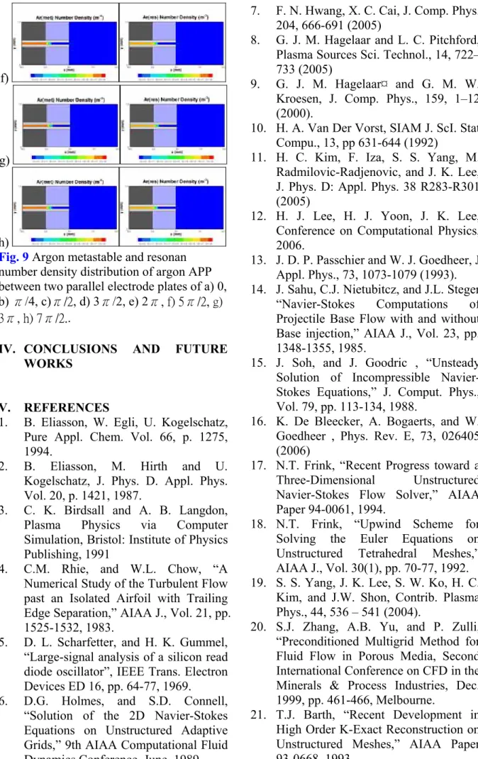
Fig. 9a shows the Ar metastable and resonan number density distribution of argon APP which the power electrode voltage just starts to rise.

Fig. 9b shows the Ar metastable and resonan number density distribution of argon APP which the voltage reaches 150V at the powered electrode.

Fig. 9c shows the Ar metastable and resonan number density distribution of argon APP which the voltage reaches the positive peak value of 300V at the powered electrode.

Fig. 9d shows the Ar metastable and resonan number density distribution of argon APP which the voltage reduces from

the positive peak value down to 150V at the powered electrode.

Fig. 9e shows the Ar metastable and resonan number density distribution of argon APP which the voltage reduces from 150V down to 0V at the powered electrode.

Fig. 9f shows the Ar metastable and resonan number density distribution of argon APP which the voltage reduces from 0V down to -150V at the powered electrode.

Fig. 9g shows the Ar metastable and resonan number density distribution of argon APP which the voltage reaches the negative peak value of -300V at the powered electrode.

Fig. 9h shows the Ar metastable and resonan number density distribution of argon APP which the voltage increases from negative peak value to -150V at the powered electrode. a) b) c) d) e)

f)

g)

h)

Fig. 9 Argon metastable and resonan

number density distribution of argon APP between two parallel electrode plates of a) 0, b) π/4, c)π/2, d) 3π/2, e) 2π, f) 5π/2, g) 3π, h) 7π/2..

IV. CONCLUSIONS AND FUTURE WORKS

V. REFERENCES

1. B. Eliasson, W. Egli, U. Kogelschatz, Pure Appl. Chem. Vol. 66, p. 1275, 1994.

2. B. Eliasson, M. Hirth and U. Kogelschatz, J. Phys. D. Appl. Phys. Vol. 20, p. 1421, 1987.

3. C. K. Birdsall and A. B. Langdon, Plasma Physics via Computer Simulation, Bristol: Institute of Physics Publishing, 1991

4. C.M. Rhie, and W.L. Chow, “A Numerical Study of the Turbulent Flow past an Isolated Airfoil with Trailing Edge Separation,” AIAA J., Vol. 21, pp. 1525-1532, 1983.

5. D. L. Scharfetter, and H. K. Gummel, “Large-signal analysis of a silicon read diode oscillator”, IEEE Trans. Electron Devices ED 16, pp. 64-77, 1969.

6. D.G. Holmes, and S.D. Connell, “Solution of the 2D Navier-Stokes Equations on Unstructured Adaptive Grids,” 9th AIAA Computational Fluid Dynamics Conference, June, 1989.

7. F. N. Hwang, X. C. Cai, J. Comp. Phys., 204, 666-691 (2005)

8. G. J. M. Hagelaar and L. C. Pitchford, Plasma Sources Sci. Technol., 14, 722– 733 (2005)

9. G. J. M. Hagelaar¤ and G. M. W. Kroesen, J. Comp. Phys., 159, 1–12 (2000).

10. H. A. Van Der Vorst, SIAM J. ScI. Stat. Compu., 13, pp 631-644 (1992)

11. H. C. Kim, F. Iza, S. S. Yang, M. Radmilovic-Radjenovic, and J. K. Lee, J. Phys. D: Appl. Phys. 38 R283-R301 (2005)

12. H. J. Lee, H. J. Yoon, J. K. Lee, Conference on Computational Physics, 2006.

13. J. D. P. Passchier and W. J. Goedheer, J. Appl. Phys., 73, 1073-1079 (1993). 14. J. Sahu, C.J. Nietubitcz, and J.L. Steger,

“Navier-Stokes Computations of Projectile Base Flow with and without Base injection,” AIAA J., Vol. 23, pp. 1348-1355, 1985.

15. J. Soh, and J. Goodric , “Unsteady Solution of Incompressible Navier-Stokes Equations,” J. Comput. Phys., Vol. 79, pp. 113-134, 1988.

16. K. De Bleecker, A. Bogaerts, and W. Goedheer , Phys. Rev. E, 73, 026405 (2006)

17. N.T. Frink, “Recent Progress toward a Three-Dimensional Unstructured Navier-Stokes Flow Solver,” AIAA Paper 94-0061, 1994.

18. N.T. Frink, “Upwind Scheme for Solving the Euler Equations on Unstructured Tetrahedral Meshes,” AIAA J., Vol. 30(1), pp. 70-77, 1992. 19. S. S. Yang, J. K. Lee, S. W. Ko, H. C.

Kim, and J.W. Shon, Contrib. Plasma Phys., 44, 536 – 541 (2004).

20. S.J. Zhang, A.B. Yu, and P. Zulli, “Preconditioned Multigrid Method for Fluid Flow in Porous Media, Second International Conference on CFD in the Minerals & Process Industries, Dec. 1999, pp. 461-466, Melbourne.

21. T.J. Barth, “Recent Development in High Order K-Exact Reconstruction on Unstructured Meshes,” AIAA Paper 93-0668, 1993.

22. T.J. Barth, and D.C. Jespersen, “The Design and Application of Upwind Schemes on Unstructured Meshes,” AIAA Paper 89-0366, 1989.

23. U. Kogelschatz, “Filamentar, Patterned, and Diffuse Barrier Discharges,” IEEE Transactions Plasma Science, Vol. 30, pp. 1810-1828, 2002.

24. U. Kogelschatz, Advanced ozone generation. In Process Technology for Water Treatment (S. Stucki, ed.), p. 87, Plenum Press, New York (1988).

25. U. Kogelschatz, B. Eliasson and W. Egli, “From ozone generators to flat television screens: history and future potential of dielectric-barrier discharges,” Pure Appl. Chem., Vol. 71, pp. 1819-2828, 1999.

26. U. Kogelschatz, XVI. International Conference on Phenomena in Ionized Gsaes, Invited Papers, p. 240, Dusseldorf, 1983.

27. U. Kogelschatz, XXIII. International Conference on Phenomena in Ionized Gsaes, Invited Papers, p. C4-47, Toulouse, 1997.

28. V.G. Samoilovich, V.I. Gibalov and K.V. Kozlov, Physical Chemistry of the Barrier Discharge, DVS-Verlag GmbH, Dusseldorf, 1997 (J.P.F. Conrads, F. Leipold, eds). Original Russian Edition, Moscow State University (1989).

29. X. C. Cai, M. A. Casarin, F. W. Elliott, Jr, and O. B. Widlund, Proceedings of the 10th Intl. Conf. on Domain Decomposition Methods (1998)

30. X. C. Cai, W. D. Gropp, D. E. Keyes, and M. D. Tidriri, Proceedings of the 7th Intl. Conf. on Domain Decomposition Methods (1994).

31. Y. Saad and M. H. Schultz, SIAM J. ScI. Stat. Compu., 7, 856-869 (1986) 32. Y.S. Chen, “An Unstructured Finite

Volume Method for Viscous Flow Computations”, 7th International Conference on Finite Element Methods in Flow Problems, Feb. 3-7, 1989, University of Alabama in Huntsville, Huntsville, Alabama.

33. Y.S. Chen, “UNIC-UNS USER’S MANUAL”, 2000.