Valuation of Standard Options under the Constant Elasticity of
Variance Model
Richard Lu*
Department of Insurance, Feng Chia University, Taiwan Yi-Hwa Hsu
Merry Electronics Co., Ltd., Taiwan
Abstract
A binomial model is developed to value options when the underlying process follows the constant elasticity of variance (CEV) model. This model is proposed by Cox and Ross (1976) as an alternative to the Black and Scholes (1973) model. In the CEV model, the stock price change ( dS ) has volatility / 2
Sβ
σ instead of σ in the Black-Scholes model. S The rationale behind the CEV model is that the model can explain the empirical bias exhibited by the Black-Scholes model, such as the volatility smile. The option pricing formula when the underlying process follows the CEV model is derived by Cox and Ross (1976), and the formula is further simplified by Schroder (1989). However, the closed-form formula is useful in some limited cases. In this paper, a binomial process for the CEV model is constructed to yield a simple and efficient computation procedure for practical valuation of standard options. The binomial option pricing model can be employed under general conditions. Also, on average, the numerical results show the binomial option pricing model approximates better than other analytic approximations.
Key words: binomial model; constant elasticity of variance model; option pricing JEL classification: G13
1. Introduction
Black and Scholes (1973) derive the well-known option pricing formula by assuming the underlying stock price follows a geometric Brownian motion. Under this construction, the price distribution is lognormal, and ignoring the time effect, the volatility is constant. However, in general, empirical evidence neither supports the lognormal distribution nor the constant volatility. In applications, the existence of a volatility smile may be the empirical bias exhibited by the underlying process in
Received July 16, 2004, revised June 9, 2005, accepted July 23, 2005. *
Correspondence to: Department of Insurance, College of Business, Feng Chia University, 100 Wenwha Rd., Taichung, Taiwan 407. E-mail: [email protected]. We are grateful to Jin-Ping Lee and the anonymous referees for their comments and suggestions.
the Black-Scholes model. To deal with this problem, many authors have suggested alternative underlying processes, such as Merton’s (1976) jump-diffusion model, Cox and Ross’s (1976) CEV model, and many stochastic volatility models.
The focus of this paper is the CEV model, which is a simple way to generalize the geometric Brownian motion in the Black-Scholes model. Following Black and Scholes (1973), Cox and Ross (1976) derive the European option pricing formula under the CEV model. Schroder (1989) shows this formula can be expressed in terms of the non-central chi-square distribution function, analogous to the standard normal distribution function in the Black-Scholes model. Since computations involving the non-central chi-square distribution function are more complicated, Schroder (1989) also provides an analytic approximation CEV option pricing formula in term of the standard normal distribution function.
The main feature of the CEV model is that it allows the volatility to change with the underlying price. As documented in Beckers (1980) and Schroder (1989), there are theoretical arguments for and empirical evidence that volatility changes with stock prices. Also, several studies support the CEV pricing model instead of the Black-Scholes pricing model (MacBeth and Merville, 1980; Emanuel and Macbeth, 1982). However, the CEV closed-form pricing formula involving the evaluation of the non-central chi-square distribution function and the analytic approximation method using the standard normal distribution function are only for European options, which can only be exercised at maturity, and not for American options, which can be exercised earlier.
The aim of this paper is to develop a simple binomial option pricing model when the underlying price process follows the CEV model. As shown in Cox et al. (1979), the early exercise valuation problem can be solved in the binomial framework. The binomial model was originally developed to approximate the normal distribution under a multiperiod setting in Cox et al. (1979). By choosing a proper transformation function, the binomial model can also be used to approximate the non-central chi-square distribution. This paper provides numerical results and compares the computational accuracy with an analytic approximation method.
The rest of this paper is organized as follows. Section 2 presents the CEV model and some versions of the CEV option pricing formula. In Section 3, a discrete-time binomial process of the CEV model is developed. Section 4 presents numerical results from the binomial option pricing model and the analytic approximation method. Finally, Section 5 concludes.
2. The CEV Model and the CEV Option Pricing Formula
The CEV model extends the Black-Scholes model to allow for stochastic volatility with a closed-form solution for option pricing. In the CEV model, the stock price is assumed to be governed by the diffusion process:
/ 2
where μ , σ , and β are parameters for growth rate, volatility, and elasticity, respectively, and w is a Wiener process. If β =2, the CEV model is just the geometric Brownian motion model. If β<2, the volatility increases as the stock price decreases. This kind of probability distribution is similar to that observed for equities with a heavy left tail and a less heavy right tail. Thus, our analysis considers the situation when β<2.
Considering a stock option with strike price K and time to maturity T−t in a constant interest rate r economy, the CEV call option pricing formula when
2 <
β in its Cox’s original form is as follows:
⎥ ⎦ ⎥ ⎢ ⎣ ⎢ + − + + − ⎥ ⎦ ⎥ ⎢ ⎣ ⎢ − + + + =
∑
∑
∞ = − − ∞ = 0 ) ( 0 ) 1 ' ( ) 2 1 1 ' ( ) 2 1 1 ' ( ) 1 ' ( j t T r j t j K G j S g e j K G j S g S Cβ
β
where . ) ( ) ( ) ( ) ( , ) 1 )( 2 ( 2 , ' ' 1 ) 2 ( ) ( 2 2 ) 2 ( ) ( 2 dy m y g m x G m x e m x g e r k k K K k e S S x m x t T r t T r∫
∞ − − − − − − − − − = Γ = − − = = = β β β β β σSchroder (1989) shows that this option pricing formula can be expressed in terms of the non-central chi-square distribution function:
⎥ ⎦ ⎥ ⎢ ⎣ ⎢ − − − − + = − ,2 ') 2 2 ; ' 2 ( 1 ) ' 2 , 2 2 2 ; ' 2 ( K S e K Q S K Q S C rt t t β β ,
where Q(z;v,k) is a complementary non-central chi-square distribution function with z, v , and k the evaluation point of the integral, degrees of freedom, and non-centrality parameter. For evaluating the distribution function, Schroder (1989) presents a simple and efficient algorithm for computation. Although the CEV option formula can be represented in terms of non-central chi-square distributions that are easier to interpret, the evaluation of an infinite sum of these distributions can be computationally slow. The algorithm suggested for computing Q(2z;2v,2k) may
converge slowly when z and k are large. Furthermore, to make this pricing formula useful, the parameter β must be equal to some specific value such that the degrees of freedom is an integer in the non-central chi-square distribution. A number of approximations to the non-central chi-square distribution have been developed. One particularly good approximation is derived by Sankaran (1963):
[ ] 1 1 0.5(2 ) ( ; , ) ~ 2 (1 ) h z hp h h mp v k Q z v k h p mp ⎛ ⎛ ⎞ ⎟⎞ ⎜ ⎜ ⎟ ⎟ ⎜ − − + − −⎜ ⎟ ⎟ ⎜ ⎜⎝ ⎟⎠ ⎟ ⎜ + ⎟ ⎜ ⎟ Φ ⎜⎜ ⎟⎟ + ⎟ ⎜ ⎟ ⎜ ⎟ ⎜ ⎟⎟ ⎜⎝ ⎠ , where 2 2 1 (2 / 3)( )( 3 )( 2 ) , 2 , ( ) ( 1)(1 3 ), h v k v k v k v k p v k m h h − = − + + + + = + = − −
and Φ is the standard normal distribution function.
3. A Binomial CEV Model
In this section, a general method for constructing binomial models proposed by Nelson and Ramaswamy (1990) is adopted. To approximate the CEV diffusion process with a binomial model, the interval
[ ]
t T, is divided into n equal pieces, each of width Δt. Over each time increment, the stock price can either increase to a particular level or decrease to another level. For the CEV model, the volatility is not constant but varies with the level of the underlying price. When the volatility varies with the level of the price, the probability of an upward move has to be recomputed at each node.At the beginning, we need to transform the diffusion process to one in which the volatility is constant and then approximate the transformed process by a simple lattice. Finally, we have to modify the probabilities on the lattice when their computed values are negative or exceed one.
Assume the stock price follows the CEV diffusion process given by: dw
S Sdt
dS =
μ
+σ
1−α ,where α =1−β 2. Considering the process x=Sα ασ and using Ito’s lemma we have:
. 2 ) 1 ( ) ( ) 1 ( 2 1 ) ( 2 1 1 2 1 2 1 2 1 2 2 dt dS S dt S S dS S dt S S x dt t x dS S x dx σ α σ σ σ α σ σ α α α α α − + = − + = ∂ ∂ + ∂ ∂ + ∂ ∂ = − − − − − (1)
Substituting into the above equation and using the fact that ασ 1α
) (x S= , Equation (1) becomes: . ) 2 ) 1 ( ( 2 ) 1 ( ) ( 2 ) 1 ( 1 1 1 dw dt x dt dS x dt dS S dx + − + = − + = − + = − − σ α αμ σ α σ ασ σ α σ α α (2)
Through transformation, this results in a new process with a constant volatility equal to 1.
Next, a binomial approximation is made to the transformed process. In each increment the approximation to Equation (2) is given by:
x+ =x+ Δt
x
x− =x− Δt.
Given the values on the x lattice, we can recover the dynamics of the stock price on its lattice: S+ = f(x+) ) (x f S= S− = f(x−).
t x x++= ++ Δ x+ =x+ Δt x x+−=x x−=x− Δt x−− =x−− Δt . Equivalently, we could construct the lattice for the S values:
) ( ++ + + = x f S S+ = f(x+) ) (x f S= S+−= f(x) S− = f(x−) ) ( −− − − = x f S .
The risk-neutral probability of an upward move depends on the level of S and the values of S+ and S− . The risk-neutral probability of an upward move is calculated by: − + − Δ − − = S S S Se P t r u . 4. Numerical Results
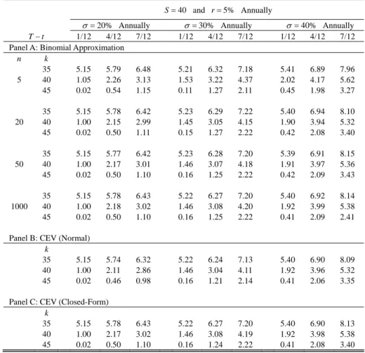
Based on the examples in Cox et al. (1979), numerical results for checking the model performances are presented in Tables 1 and 2. We choose α equal to 0.1 and 0.5 because the two numbers can fit into Schroder’s (1989) formula, which requires integer degrees of freedom in the complementary non-central chi-square distribution function. The stock price is 40 and the interest rate is 5%. The values of
σ in the CEV model are chosen such that the annual standard deviations of stock returns equal 0.2, 0.3, and 0.4. These parameter values are the same as in Cox et al. (1979). Furthermore, an approximate analytic solution using the normal distribution function is given for comparison.
As with other binomial applications, the values of the options converge quickly to the closed-form solutions as the number of steps n increases. When n=20, on average, the value from the binomial option pricing model is closer to the closed-form solutions than the approximate analytic solution using the normal distribution function. For n=50, the numerical results show that the difference between the binomial model the closed-form formula is less than or equal to 0.02. However, the results from the approximate analytic solution show larger deviation,
especially for longer maturity. For instance, when the time to maturity is 7 months and the annual standard deviation is 20%, the value of the at-the-money option is 2.86 by the approximate analytic solution, while the closed-form solution is 3.02.
Table 1. Values of European Call Options on Stock for the CEV Process (α=0.5)
40 = S and r=5% Annually % 20 =
σ Annually σ=30% Annually σ=40% Annually
t
T− 1/12 4/12 7/12 1/12 4/12 7/12 1/12 4/12 7/12 Panel A: Binomial Approximation
n k 35 5.15 5.82 6.51 5.22 6.37 7.23 5.44 6.95 8.08 5 40 1.05 2.26 3.13 1.53 3.22 4.37 2.02 4.17 5.62 45 0.01 0.50 1.10 0.10 1.22 2.05 0.42 1.91 3.15 35 5.15 5.80 6.46 5.23 6.34 7.29 5.43 7.01 8.21 20 40 1.00 2.15 2.99 1.45 3.05 4.16 1.90 3.94 5.33 45 0.02 0.48 1.05 0.14 1.21 2.14 0.39 2.01 3.29 35 5.15 5.79 6.46 5.23 6.33 7.26 5.42 6.99 8.26 50 40 1.00 2.17 3.01 1.46 3.07 4.18 1.91 3.97 5.36 45 0.02 0.47 1.05 0.14 1.20 2.14 0.39 2.01 3.32 35 5.15 5.80 6.46 5.24 6.32 7.28 5.42 7.00 8.25 1000 40 1.00 2.18 3.02 1.46 3.07 4.20 1.92 3.99 5.39 45 0.02 0.47 1.05 0.15 1.19 2.14 0.39 2.01 3.30 Panel B: CEV (Normal)
k
35 5.15 5.78 6.39 5.24 6.32 7.27 5.42 7.02 8.29 40 1.00 2.13 2.92 1.46 3.07 4.19 1.92 4.01 5.43 45 0.02 0.44 0.97 0.14 1.18 2.13 0.39 2.02 3.34 Panel C: CEV (Closed-Form)
k
35 5.15 5.79 6.44 5.23 6.31 7.26 5.42 6.99 8.23 40 1.00 2.17 3.00 1.46 3.07 4.19 1.92 3.98 5.37 45 0.02 0.47 1.04 0.14 1.18 2.13 0.38 2.00 3.29 Notes: S denotes spot price; r represents interest rate; k , t, and n indicates strike price, time to maturity, and the number of steps in the binomial model, respectively. The value of σ is set such that the annual standard deviations σ are 0.2, 0.3, and 0.4 at the spot price 40. The option values in Panel B are calculated with the approximate analytic formula using the normal distribution function. The option values in Panel C are the closed-form solutions for the CEV process.
In additional to the numerical example in Cox et al. (1979), we consider numerical results when the stock price equals either 30 or 40 and the interest rate equals 2% or 8% to check the robustness of the results. Comparing the three models, the accuracy of results is similar to Tables 1 and 2. As a consequence, the additional results are not reported here (but are available from the authors upon request).
Table 2. Values of European Call Options on Stock for the CEV Process (α=0.1) 40 = S and r=5% Annually % 20 =
σ Annually σ=30% Annually σ=40% Annually
t
T− 1/12 4/12 7/12 1/12 4/12 7/12 1/12 4/12 7/12 Panel A: Binomial Approximation
n k 35 5.15 5.79 6.48 5.21 6.32 7.18 5.41 6.89 7.96 5 40 1.05 2.26 3.13 1.53 3.22 4.37 2.02 4.17 5.62 45 0.02 0.54 1.15 0.11 1.27 2.11 0.45 1.98 3.27 35 5.15 5.78 6.42 5.23 6.29 7.22 5.40 6.94 8.10 20 40 1.00 2.15 2.99 1.45 3.05 4.15 1.90 3.94 5.32 45 0.02 0.50 1.11 0.15 1.27 2.22 0.42 2.08 3.40 35 5.15 5.77 6.42 5.23 6.28 7.20 5.39 6.91 8.15 50 40 1.00 2.17 3.01 1.46 3.07 4.18 1.91 3.97 5.36 45 0.02 0.50 1.10 0.16 1.25 2.22 0.42 2.09 3.43 35 5.15 5.78 6.43 5.22 6.27 7.20 5.40 6.92 8.14 1000 40 1.00 2.18 3.02 1.46 3.08 4.20 1.92 3.99 5.38 45 0.02 0.50 1.10 0.16 1.25 2.22 0.41 2.09 2.41 Panel B: CEV (Normal)
k
35 5.15 5.74 6.32 5.22 6.24 7.13 5.40 6.90 8.09 40 1.00 2.11 2.86 1.46 3.04 4.11 1.92 3.96 5.32 45 0.02 0.46 0.98 0.16 1.21 2.14 0.41 2.06 3.35 Panel C: CEV (Closed-Form)
k
35 5.15 5.78 6.43 5.22 6.27 7.20 5.40 6.90 8.13 40 1.00 2.17 3.02 1.46 3.08 4.19 1.92 3.98 5.38 45 0.02 0.50 1.10 0.16 1.24 2.22 0.41 2.08 3.40 Notes: S denotes spot price; r represents interest rate; k , t, and n indicates strike price, time to maturity, and the number of steps in the binomial model, respectively. The value of σ is set such that the annual standard deviations σ are 0.2, 0.3, and 0.4 at the spot price 40. The option values in Panel B are calculated with the approximate analytic formula using the normal distribution function. The option values in Panel C are the closed-form solutions for the CEV process.
5. Conclusion
In this paper, we follow a general method for constructing binomial models to develop a binomial lattice for pricing options when the underlying process follows the CEV model. The CEV model was proposed by Cox and Ross (1976) as a more general alternative to the Black and Scholes (1973) model. In the CEV model, the stock price can exhibit volatility changes with the price level. The motivation behind the CEV model is that it can explain the empirical bias exhibited by the Black-Scholes model, such as a volatility smile. Though the CEV closed-form pricing formula and the analytic approximation method for CEV option pricing have
been developed, they are only for European-style options and not for American-style options.
In this paper, a binomial process for the CEV model is constructed to yield a simple and efficient computational procedure for practical valuation of standard options. This binomial option pricing model can be used for options with early exercise features. On average, the numerical results show the binomial option pricing model approximates well compared with the analytic approximation method.
References
Black, F. and M. Scholes, (1973), “The Pricing of Options and Corporate Liabilities,” Journal of Political Economy, 81, 637-654.
Beckers, S., (1980), “The Constant Elasticity of Variance Model and Its Implications for Option Pricing,” Journal of Finance, 35, 661-673.
Cox, J. C. and S. A. Ross, (1976), “The Valuation of Options for Alternative Stochastic Processes,” Journal of Financial Economics, 3, 145-166.
Cox, J. C., S. A. Ross, and M. Rubinstein, (1979), “Option Pricing: A Simplified Approach,” Journal of Financial Economics, 7, 229-263.
Cox, J. C. and M. Rubinstein, (1985), Option Markets, Englewood Cliffs, NJ: Prentice-Hall.
Emanuel, D. C. and J. D. MacBeth, (1982), “Further Results on the Constant Elasticity of Variance Call Option Pricing Model,” Journal of Financial and
Quantitative Analysis, 17, 533-554.
MacBeth, J. D. and L. J. Merville, (1980), “Tests of the Black-Scholes and Cox Call Option Valuation Models,” Journal of Finance, 35, 285-301.
Merton, R. C., (1976), “Option Pricing when Underlying Stock Returns are Discontinuous,” Journal of Financial Economics, 3, 125-144.
Sankaran, M., (1963), “Approximations to the Non-Central Chi-Square Distribution,”
Biometrika, 50, 199-204.
Schroder, M., (1989), “Computing the Constant Elasticity of Variance Option Pricing Formula,” Journal of Finance, 44, 211-219.