An Improved Weighted Clustering Algorithm for Determination of Application Nodes in Heterogeneous Sensor Networks

An Improved Weighted Clustering Algorithm for

Determination of Application Nodes in Heterogeneous

Sensor Networks

Tzung-Pei Hong1,2 and Cheng-Hsi Wu3

1

Department of Computer Science and Information Engineering National University of Kaohsiung

2

Department of Computer Science and Engineering, National Sun Yat-sen University

3

Department of Electrical Engineering, National University of Kaohsiung Kaohsiung, Taiwan, R.O.C.

E-mail: [email protected], [email protected]

Abstract

Along with the advances of internet and communication technology, mobile ad hoc networks (MANETs) and wireless sensor networks have attracted extensive research efforts in recent years. In the past, Chatterjee et al. proposed an efficient approach, called the weighted clustering algorithm, to determine the cluster heads dynamically in mobile ad hoc networks. Wireless sensor networks are, however, a little different from traditional networks due to some more constraints. Besides, in wireless sensor networks, prolonging network lifetime is usually an important issue. In this paper, an improved algorithm based on the weighted clustering algorithm is proposed with additional constraints for selection of cluster heads in mobile wireless sensor networks. The cluster heads chosen will act as the application nodes in a two-tired wireless sensor network and may change in different time intervals. After a fixed interval of time, the proposed algorithm is re-run again to find new applications nodes such that the system lifetime can be expected to last longer. Experimental results also show the proposed algorithm behaves better than Chatterjee’s on wireless sensor networks for long system lifetime.

Keywords: mobile ad hoc network, wireless sensor network, two-tiered

1.

Introduction

Along with the advances of internet and communication technology, mobile ad hoc networks (MANETs) and wireless sensor networks have attracted extensive research efforts in recent years [1][23]. In the past, many approaches were proposed to efficiently handle the problems of path routing, node clustering, dynamic scheduling, among others in mobile ad hoc networks [4][6][11][12][19][24]. For example, appropriate transmission ways were designed for multi-hop communication in ad-hoc networks [7][14][22]. Wireless sensor networks are, however, a little different from traditional networks due to some more constraints. Especially, the former must usually take the energy factor into consideration in order to prolong the network lifetime [8][20]. Efficiently utilizing energy in wireless sensor networks thus becomes an important research topic in this area. Good algorithms for allocation of base stations and sensors nodes were then proposed to reduce power consumption [10][13][15][20].

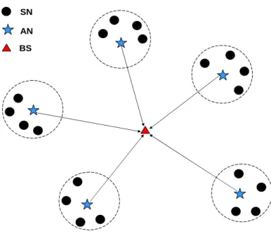
Sensors in a wireless sensor network can not only collect data from an environment but can also process data and transmit information. Recently, a two-tiered architecture of wireless sensor networks has been proposed and become popular [5][25]. It is motivated by the latest advances in distributed signal processing and source coding and can offer a more flexible balance among reliability, redundancy and scalability of wireless sensor networks. A two-tiered wireless sensor network, as shown in Figure 1, consists of sensor nodes (SNs), application nodes (ANs), and one or several base stations (BSs).

SN AN BS

Figure 1: A two-tiered architecture of wireless sensor networks

Sensor nodes are usually small, low-cost and disposable, and do not communicate with other sensor nodes. They are usually deployed in clusters around interesting areas. For instance, sensor nodes may be used to detect a designated target, environment temperature and humidity, among others. Each cluster of sensor nodes is allocated with at least one application node. Application nodes possess longer-range transmission, higher-speed computation, and more energy than sensor nodes. The raw data obtained from sensor nodes are first transmitted to their corresponding application nodes. After receiving the raw data from all its sensor nodes, an application node conducts data fusion within each cluster. It then transmits the aggregated data directly to the base station or via multi-hop communication. The base station is usually assumed to have unlimited energy and powerful processing capability. It also serves as a gateway for wireless sensor networks to exchange data and information to other networks. Wireless sensor networks usually have some assumptions for SNs and ANs. For instance, each AN may be aware of its own location through receiving GPS signals [15] and its own energy. Many researches based on the two-tiered wireless sensor network were done. For example, Pan et al. collected information from nearby SNs for good scheduling in two-tiered wireless

of base stations in two-tiered wireless sensor networks [16][17]. Hong and Shiu also proposed an allocation scheme for base stations based on the technique of particle swarm optimization (PSO) [9].

Sensor networks may be divided into homogeneous and heterogeneous ones. All sensor nodes in a homogeneous sensor network possess the same parameters and in a heterogeneous one possess different parameters. Besides, sensors may be fixed or moveable. In this paper, heterogeneous sensor networks are considered. Sensor nodes may have different capability and different parameters. Besides, each node may act as both the roles of a sensor node and an application node. An improved algorithm based on the weighted clustering algorithm used in mobile ad hoc networks is proposed to determine the cluster heads in a given mobile wireless sensor network. The cluster heads chosen will act as the application nodes and may change in different time intervals. The power energy and the transmission rate of sensor nodes are taken into consideration in the algorithm. After a fixed interval of time, the proposed algorithm is re-run again to find new applications nodes such that the system lifetime can be expected to last longer. An example is also given and experiments are made to show the effectiveness of the proposed algorithm in wireless sensor networks for lifetime.

The remaining parts of this paper are organized as follows. The WCA approach is introduced in Section 2. An improved algorithm based on WCA for application in wireless sensor networks is proposed in Section 3. An example to illustrate the proposed algorithm is given in Section 4. Experimental results for demonstrating the performance of the algorithm is described in Section 5. Conclusions and future works are given in Section 6.

2.

Review of the Weighted Clustering Algorithm

Along with the advances of internet and communication technology, mobile ad hoc networks (MANETs) have attracted extensive research efforts in recent years. In the past, Chatterjee et al. proposed the weighted clustering algorithm (WCA) for identifying cluster heads in mobile ad-hoc networks [2][3]. A mobile ad hoc network can be modeled as composing of nodes and links, which is usually represented by a

graph G =(V,E), where V represents the set of nodes and E represents the set of

links. They assume the transmission radii for all nodes are the same. The following formula is used to calculate the combined weight (Wv) of a node v as a cluster head:

v v v v v w w D w M wT W = 1∆ + 2 + 3 + 4 ,

where v is the serial number (ID) of a mobile node, △v is the degree difference of

node v, Dv is the sum of the distances between v and its neighbors, Mv is the mobility

speed of node v, Tv is the cumulative time in which node v acted as a cluster head, and

wi is the weighted coefficient for the i-th factor. The degree of a node v is the number

of nodes within its transmission radius, not including itself. The degree difference is thus the difference between the degree of a node v and a predefined ideal node

number M in a cluster. Wv is used to determine the goodness of a node as a cluster

head. The lower the Wv value is, the better v acts as a cluster head. The details of the

weighted clustering algorithm are described below:

The Weighted Clustering Algorithm:

Input: A set of sensor nodes, each with the same transmission radius Rv, its individual

cumulative time Tv and mobility speed Mv, the predefined ideal node number

M in a cluster, and the four coefficients w1 to w4.

Output: A set of cluster heads with its neighbors.

Step 1: Find the neighbors N(v) of each node v, where a neighbor is a node with its

distance with v within the transmission radius Rv. That is:

} ) ' , ( distance |' { ) (v v v v Rv N = ≤ .

Calculate the degree dv of node v as the number of the neighbors of v.

Step 2: Compute the degree difference △v as |dv – M| for every node v.

Step 3: Compute the sum Dv of the distances between node v with all its neighbors. That

is:

∑

(

) (

)

∑

where (Xt, Yt) and (Xt-1, Yt-1) are the coordinate positions of node v at time t

and t-1.

Step 5: Find the cumulative time Tv in which node v has acted as a cluster head. A larger

Tv value with node v implies that it has spent more resources (such as energy).

Step 6: Calculate the combined weight W_v =w₁∆_v +w₂D_v +w₃M_v +w₄T_v for every node v.

Step 7: Choose the node with a minimum Wv as the cluster head.

Step 8: Eliminate the chosen cluster head and its neighbors from the set of original sensor nodes.

Step 9: Repeat Steps 1 to 8 for the remaining nodes until each node is assigned to a cluster.

After Step 9, all the mobile nodes can be grouped into several clusters, and each cluster has its cluster head. Sensor networks in general have more constraints (such as the energy) than traditional networks. In this paper, we will modify the weighted clustering algorithm such that it can be used in sensor networks with their specific constraints considered.

3. The Proposed Approach

The WCA algorithm was designed to select cluster heads dynamically in mobile ad hoc networks. As mentioned above, sensor networks in general have more constraints than traditional networks. It is thus not so appropriate to directly apply the WCA algorithm to the sensor networks since it does not take the power energy, the transmission rate, among others into consideration. In this paper, we will modify the weighted clustering algorithm such that it can be used in sensor networks with the specific constraints in sensor networks being considered. Especially, we add one more factor about the characteristic of a sensor node into the evaluation formula, such that the nodes chosen as cluster heads may have a better behavior in heterogeneous sensor networks than those without the additional factor. The cluster heads can then act as

application nodes in the sensor networks. After a fixed interval of time, the proposed algorithm is then re-run again to find new applications nodes for the purpose of getting a longer system lifetime. The details of the improved WCA algorithm for heterogeneous sensor networks are stated below.

The improved WCA algorithm (IWCA) for heterogeneous sensor networks:

Input: A set of sensor nodes, each with the same transmission radius Rv, its individual

cumulative time Tv, mobility speed Mv, transmission rate rv, the initial energy

Ev, the constant of amplification c the predefined ideal node number M in a

cluster, and the five coefficients w1 to w5.

Output: A set of application nodes with its neighbors.

Step 1: Find the neighbors N(v) of each node v, where a neighbor is a node with its distance with v within the transmission radius Rv. That is:

} ) ' , ( distance |' { ) (v v v v Rv N = ≤ .

Calculate the degree dv of node v as the number of the neighbors of v.

Step 2: Compute the degree difference △v as |dv – M| for every node v.

Step 3: Compute the sum Dv of the distances between node v with all its neighbors. That

is:

∑

Step 4: Compute the mobility speed of every node v by the following formula:

(

) (

)

∑

where (Xt, Yt) and (Xt-1, Yt-1) are the coordinate positions of node v at time t and t-1.

Step 5: Find the cumulative time Tv in which node v has acted as a cluster head. A larger

Tv value with node v implies that it has spent more resources (such as energy).

Step 6: Compute the characteristic Cv of every node v as follows:

v v v E r c C = * ,

where rv is the transmission rate, Ev is the initial energy and c is a constant for

Step 7: Calculate the combined weight W_v =w₁∆_v+w₂D_v +w₃M_v +w₄T_v +w₅C_v for every node v.

Step 8: Choose the node with a minimum Wv as the cluster head (application node).

Step 9: Eliminate the chosen cluster head and its neighbors from the set of original sensor nodes.

Step 10:Repeat 1 to 9 for the remaining nodes until each node is assigned to a cluster.

Note that in Step 6, the factor for the characteristic of a node is added to evaluate the goodness of a node as a cluster head. As an alternative to evaluate the goodness of a node, the factor of the cumulative time can be removed and the initial energy in the characteristic factor of a node can be changed as the remaining energy. This is because the remaining energy of a node partially depends on its cumulative time as a cluster head.

4. An Example

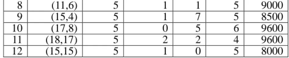
A simple example in a two-dimensional space is given to explain how the IWCA can be used to find the application nodes in dynamic wireless sensor networks. Assume in this example there are totally twelve mobile sensor nodes activated with their initial factors shown in Table 3, where “SN” represents the series number of a sensor node, “Location” represents the coordinate position of an SN, “Radius” represents the transmission radius, “Mobility” represents the mobility speed, “Time” represents the cumulative time, “Rate” represents the transmission rate, and “Energy” represents the initial power energy.

Table 3: The initial factors of SNs in the example

SN Location Radius Mobility Time Rate Energy

1 (3,3) 5 2 1 5 7500 2 (4,7) 5 2 2 6 7200 3 (4,12) 5 1 4 6 6600 4 (7,15) 5 1 6 4 8400 5 (11,15) 5 2 0 5 10000 6 (15,20) 5 3 2 4 7600 7 (7,4) 5 4 1 4 9600

8 (11,6) 5 1 1 5 9000

9 (15,4) 5 1 7 5 8500

10 (17,8) 5 0 5 6 9600

11 (18,17) 5 2 2 4 9600

12 (15,15) 5 1 0 5 8000

Besides, some required parameters have to be set for the improved weighted clustering algorithm (IWCA) to work. In this example, the threshold number M is set at 3, which means an application node can ideally handle 3 sensor nodes. The five coefficient values are set as follows: w1=0.5, w2=0.1, w3=0.05, w4=0.05 and w5=0.3

where the summation of the weights is equal to 1. For this example, the proposed algorithm proceeds as follows. Only the first SN is demonstrated to show the execution process.

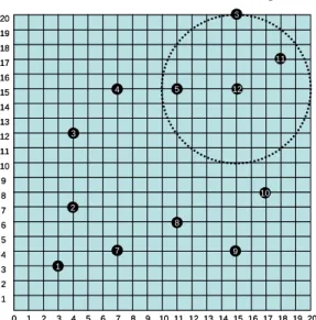
Step 1: The neighbors of every sensor node v are searched and its degree dv is

obtained. The results are shown in Figure 2, where the neighbors of SN1 are SN2 and SN7. The degree d1 is thus 2.

19 20 18 17 16 15 14 13 12 11 10 9 8 7 6 5 4 3 2 1 0 1 2 3 4 5 6 7 8 9 10111213 14151617 1819 20 0 1 2 3 4 5 6 7 8 9 10 11 12 13 14 15 16 17 18 19 20 1 2 3 4 5 6 7 8 9 10 11 12 13 14 15 16 17 18 19 20 1 2 2 3 3 4 4 55 6 6 7 7 8 8 9 9 10 10 11 11 12 12

Figure 2: The neighbors of each SN in the example

Step 2: The degree difference of every node v is computed by the formula

M dv

v = −

∆ . Assume in this example, M=3. The degree difference of SN1 is

Step 3: The sum of the distances Dv between an SN and all its neighbors is

calculated. For SN1, D₁=

(

) (

)

(

) (

)

example, assume in the past 2 time blocks, SN 1 has moved from the position (1, 1) to (1, 3) and then to (3, 3). Its mobility speed is calculated as follows:

( ) ( )

( ) ( )

Step 5: The cumulative time Tv for a node v to act as an application node is

obtained. Assume the cumulative time obtained so far is shown in the column Tv of

Table 4.

Step 6: The characteristic Cv of every node v is derived. Assume in this

example, the constant of amplification c is set at 1000. The characteristic factor for SN1 is calculated as follows: 67 . 0 7500 / 5 * 1000 / * 1 1 1 =c r E = ≅ C .

Step 7: The combined weight of each sensor node v is calculated by the

formula: v v v v v v w w D w M wT wC W = 1∆ + 2 + 3 + 4 + 5 .

For SN1, it weight is:

. 67 . 1 67 . 0 * 3 . 0 1 * 05 . 0 2 * 05 . 0 25 . 8 * 1 . 0 1 * 5 . 0 * 3 . 0 * 05 . 0 * 05 . 0 * 1 . 0 * 5 . 0 _{1 1 1 1 1} 1 = + + + + = + + + + ∆ = D M T C W

After Step 7, all the factor values for the sensor nodes are listed in Table 4.

Table 4: The factor values of the sensor nodes in this example

SN Loc Rv rv Ev dv △v Dv Mv Tv Fv Wv 1 (3,3) 5 5 7500 2 1 8.25 2 1 0.67 1.67 2 (4,7) 5 6 7200 3 0 13.37 2 2 0.83 1.79 3 (4,12) 5 6 6600 2 1 9.24 1 4 0.91 1.95 4 (7,15) 5 4 8400 2 1 8.24 1 6 0.48 1.82 5 (11,15) 5 5 10000 2 1 8.00 2 0 0.50 1.55 6 (15,20) 5 4 7600 2 1 9.24 3 2 0.53 1.83 7 (7,4) 5 4 9600 3 0 12.84 4 1 0.42 1.66 8 (11,6) 5 5 9000 2 1 8.94 1 1 0.56 1.66

9 (15,4) 5 5 8500 2 1 8.94 1 7 0.59 1.97

10 (17,8) 5 6 9600 1 2 4.47 0 5 0.63 1.88

11 (18,17) 5 4 9600 2 1 7.85 2 2 0.42 1.61

12 (15,15) 5 5 8000 3 0 12.61 1 0 0.63 1.50

Step 8: The node with a minimum W is chosen as the cluster head. It can be _v

observed from Table 4 that W12 has a minimum combined weight (1.5). SN12 is thus

chosen as an application node. The results are shown as Figure 3.

19 20 18 17 16 15 14 13 12 11 10 9 8 7 6 5 4 3 2 1 0 1 2 3 4 5 6 7 8 9 10111213141516171819 20 0 1 2 3 4 5 6 7 8 9 10 11 12 13 14 15 16 17 18 19 20 1 2 3 4 5 6 7 8 9 10 11 12 13 14 15 16 17 18 19 20 1 2 3 4 5 6 7 8 9 10 11 12

Figure 3: The first chosen application node with its neighbors

Step 9: The chosen cluster head and its neighbors are thus eliminated from the set of

original sensor nodes. The results after SN12 and its neighbors are deleted are shown in Figure 4. 19 20 18 17 16 15 14 13 12 11 10 9 8 7 6 5 4 3 2 1 0 1 2 3 4 5 6 7 8 9 10111213141516171819 20 0 1 2 3 4 5 6 7 8 9 10 11 12 13 14 15 16 17 18 19 20 1 2 3 4 5 6 7 8 9 10 11 12 13 14 15 16 17 18 19 20 1 2 3 4 7 8 9 10

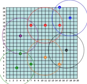
Step 10:Steps 1 to 9 are repeated for processing the remaining nodes until each node is assigned to a cluster. The final clusters are shown in Figure 5. There are totally 4 clusters formed in this example

19 20 18 17 16 15 14 13 12 11 10 9 8 7 6 5 4 3 2 1 0 1 2 3 4 5 6 7 8 9 10111213141516171819 20 0 1 2 3 4 5 6 7 8 9 10 11 12 13 14 15 16 17 18 19 20 1 2 3 4 5 6 7 8 9 10 11 12 13 14 15 16 17 18 19 20 1 2 3 4 5 6 7 8 9 10 11 12

Figure 5: The final clusters by IWCA

For a comparison, the WCA algorithm is also run for the same example. The clustering results are shown in Figure 6. More clusters are derived by WCA than by IWCA. 19 20 18 17 16 15 14 13 12 11 10 9 8 7 6 5 4 3 2 1 0 1 2 3 4 5 6 7 8 9 10111213141516171819 20 0 1 2 3 4 5 6 7 8 9 10 11 12 13 14 15 16 17 18 19 20 1 2 3 4 5 6 7 8 9 10 11 12 13 14 15 16 17 18 19 20 1 2 3 4 5 6 7 8 9 10 11 12

Figure 6: The final clusters of the given SNs by WCA

5. Experimental Results

algorithm and the original WCA algorithm on the determination of the application nodes. They were implemented in the C++ language on an AMD Athlon 64-bits PC with 1.99 GHZ CPU and 2G RAM under the Microsoft Windows XP operating system. The simulation was done in a two-dimensional real-number square space 1000*1000. The four coefficient values of WCA were set at the same values as those in the original WCA experiments [2][3]. Those are w1 = 0.7, w2 = 0.2, w3 = 0.05, and

w4 = 0.05, where the summation of the weights is equal to 1. In the IWCA algorithm,

the five coefficient values are set as w1 = 0.5, w2 = 0.1, w3 = 0.05, w4 = 0.05 and w5 =

0.3, according to the previous WCA experiments with a little adjustment for the sensor characteristics. The summation of the weights is still equal to 1. The degree threshold M is set at 100, the transmission rate was limited between 1 to 10, the range of the initial energy was limited between 10000000 to 99999999, and both the mobility speed and the cumulative time were limited between 0 to 10. The number of sensor nodes was 1000. The data of all the sensor nodes, each with its own, were thus randomly generated according to the above rules.

In the experiments, the base stations were randomly generated to compute the system lifetime from the application nodes which were clustered by IWCA and WCA respectively. The lifetime formula is the same as that in [17]. The number of base stations was simulated from 1 to 5. The transmission radius of an application node was assumed unlimited for simplifying the computation of system lifetimes. Every application node would thus choose the nearest base station and compute its lifetime. The minimum lifetime among those generated from all the application nodes was the system lifetime. The system lifetimes from the application nodes determined by the two algorithms along with different numbers of base stations were shown in Figure 7.

0 5 10 15 20 25 1 2 3 4 5 number of BSs lif et im e IWCA WCA

Figure 8: The lifetimes by the two algorithms for different numbers of base stations

It can be observed from Figure 7 that the lifetimes along with different numbers of base stations would go up steadily. In the experiments, the IWCA algorithm got better system lifetimes than the WCA algorithm. It was because IWCA took the characteristics of a sensor node into consideration, but WCA didn’t. The execution time of the two algorithms along with different numbers of base stations is shown in Figure 8. 0 2 4 6 8 10 12 1 2 3 4 5 number of BSs ex ec ut io n tim e IWCA WCA

Figure 8: The execution time of the two algorithms for different numbers of base stations

It could be observed from Figure 8 that the execution time was almost the same for IWCA and WCA. The execution time increased along with the increase of the number of base stations. The clusters obtained in the experiments were 15 to 20 approximately. There was a small difference of the numbers of application nodes for IWCA and WCA. The execution time of the two algorithms was thus about the same.

6. Conclusions

In wireless sensor networks, power consumption is an important factor for network lifetime. In this paper, we have proposed an improved clustering algorithm based on the weighted clustering algorithm with additional constraints for selection of cluster heads in mobile wireless sensor networks. The characteristics of sensor nodes including the power energy and the transmission rate are considered in the proposed algorithm. The cluster heads chosen can act as the application nodes in a two-tired wireless sensor network and may change in different time intervals. After a fixed interval of time, the proposed algorithm is re-run again to find new applications nodes such that the system lifetime can be expected to last longer. An example has also been given to illustrate the proposed algorithm in details. Experimental results have shown the proposed algorithm behaves better than Chatterjee’s on wireless sensor networks for long system lifetime. In the future, we will consider using other effective clustering approaches to the problem [21][26]. We will also attempt to extend the proposed approach to solving more complicated problems in wireless sensor networks.

References

[1] I. Akyildiz, W. Su, Y. Sankarasubramaniam, and E. Cayirci, “Wireless sensor networks: a survey”, Computer Networks, Vol. 38, No.4, pp. 393-422, 2002. [2] M. Chatterjee, S. K. Das, and D. Turgut, “An on-demand weighted clustering

algorithm (WCA) for ad hoc networks”, The IEEE Global Telecommunications

Conference, pp. 1697-1701, 2000.

[3] M. Chatterjee, S. K. Das, and D. Turgut, “WCA: a weighted clustering algorithm

for mobile ad hoc networks”, Cluster Computing, Vol. 5, No. 2, pp. 193-204, 2002.

[4] I. Chlamtac and A. Farago, “A new approach to the design and analysis of peer-to-peer mobile networks”, Wireless Networks, Vol. 5, No. 3, pp. 149-156, 1999.

processing approach to reducing energy consumption in sensor networks”, The

22nd IEEE Conference on Computer Communications, pp. 1054-1062, 2003.

[6] P. Gupta and P. R. Kumar, “The capacity of wireless networks”, IEEE

Transactions on Information Theory, Vol. 46, No. 2, pp. 388-404, 2000.

[7] W. Heinzelman, J. Kulik, and H. Balakrishnan, “Adaptive protocols for

information dissemination in wireless sensor networks”, The Fifth ACM

International Conference on Mobile Computing and Networking, pp. 174-185,

1999.

[8] W. Heinzelman, A. Chandrakasan, and H. Balakrishnan, “Energy-efficient

communication protocols for wireless microsensor networks”, The 33rd Annual

Hawaiian International Conference on Systems Science, 2000.

[9] T. P. Hong, G. N. Shiu, and Y. C. Lee, "Finding base-station locations in two-tiered wireless sensor networks by particle swarm optimization", Particle

Swarm Optimization, Chapter 16, I-Tech Education and Publishing, pp. 261-274,

2009.

[10] C. Intanagonwiwat, R. Govindan and D. Estrin, “Directed diffusion: a scalable and robust communication paradigm for sensor networks”, The ACM

International Conference on Mobile Computing and Networking, 2000.

[11] S. Jin, M. Zhou, A. S. Wu, “Sensor Network Optimization Using a Genetic Algorithm”, The 7th World Multiconference on Systemics, Cybernetics, and

Informatics, 2003.

[12] M. Joa-Ng and I. T. Lu, “A Peer-to-Peer Zone-based Two-level Link State Routing for Mobile Ad Hoc Networks”, IEEE Journal on Selected Areas in

Communications, Vol. 17, No. 8, pp. 1415-1425, 1999.

[13] V. Kawadia and P. R. Kumar, “Power control and clustering in ad hoc networks”,

The 22nd IEEE Conference on Computer Communications, pp. 459-469, 2003.

[14] S. Lee, W. Su, and M. Gerla, “Wireless ad hoc multicast routing with mobility prediction”, Mobile Networks and Applications, Vol. 6, No. 4, pp. 351-360, 2001.

[15] D. Niculescu and B. Nath, “Ad hoc positioning system (APS) using AoA”, The

22nd IEEE Conference on Computer Communications, pp. 1734-1743, 2003.

networks”, The Ninth ACM International Conference on Mobile Computing and

Networking, pp. 286-299, 2003.

[17] J. Pan, L. Cai, Y. T. Hou, Y. Shi, and S. X. Shen, "Optimal base-station locations in two-tiered wireless sensor networks", IEEE Transactions on Mobile

Computing, Vol. 4, No. 5, pp. 458-473, 2005.

[18] J. Pan, Y. T. Hou, L. Cai, Y. Shi, and S, X. Shen, “Serialized optimal relay schedules in two-tiered wireless sensor networks”, Computer Communication, Vol. 29, No.4, pp. 511-524, 2006.

[19] Y. Q. Qin, D. B. Sun, N. Li, and Y. G. Cen, “Path planning for mobile robot using

the particle swarm optimization with mutation operator”, The IEEE Third

International Conference on Machine Learning and Cybernetics, pp. 2473-2478

2004.

[20] V. Rodoplu and T. H. Meng, “Minimum energy mobile wireless networks”, IEEE

Journal on Selected Areas in Communications, Vol. 17, No. 8, pp. 1333-1344,

1999.

[21] L. Ramachandran, M. Kapoor, A. Sarkar, and A. Aggarwal, “Clustering

algorithms for wireless ad hoc networks”, The Fourth International Workshop on

Discrete Algorithms and Methods for Mobile Computing and Communications,

pp. 54-63, 2000.

[22] R. Ramanathan and R. Hain, “Topology control of multihop wireless networks using transmit power adjustment”, The 19th IEEE Conference on Computer

Communications, pp. 404-413, 2000.

[23] R. Ramanathan and J. Redi, “A brief overview of ad hoc networks: challenges and directions”, IEEE Communications Magazine, Vol. 40, pp. 20–22, 2002.

[24] D. Tian and N. Georganas, “Energy efficient Routing with guaranteed delivery in

wireless sensor networks,” The IEEE Wireless Communication & Networking

Conference, pp. 1923-1929, 2003.

[25] F. Ye, H. Luo, J. Cheng, S. Lu and L. Zhang, “A two-tier data dissemination model for large scale wireless sensor networks”, The 8th ACM International

Conference on Mobile Computing and Networking, 2002.

and its application in hierarchical community discovery”, Journal of Information