The Integer Transforms Analogous to Discrete
Trigonometric Transforms
Soo-Chang Pei, Fellow, IEEE, and Jian-Jiun Ding
Abstract—Integer transform (such as the Walsh transform)
is the discrete transform that all the entries of the transform matrix are integer. It is much easy to implement because the real number multiplication operations can be avoided, but the performance is usually worse. On the other hand, the noninteger transform, such as the DFT and DCT, has good performance, but the real number multiplication is required. In this paper, we will try to derive the integer transforms analogous to some popular noninteger transforms. These integer transforms remain most of the performance quality of the original transform, but the implementation will be much simpler. Especially, for two-di-mensional (2-D) block transform in image/video, the saving can be huge for using integer operations. In 1989, Cham had derived the integer cosine transform. Here, we will derive the integer sine, Hartley, and Fourier transforms. We also introduce the general method to derive the integer transform from some noninteger transform. Besides, the integer transform derived by Cham still requires real number multiplication for the inverse transform. We will modify the integer transform introduced by Cham and introduce the complete integer transform. It requires no real number multiplication operation, no matter what the forward or inverse transform. The integer transform we derive would be more efficient than the original transform. For example, for the 8-point DFT and IDFT, there are in total four real numbers and eight fixed-point multiplication operations required, but for the forward and inverse 8-point complete integer Fourier transforms, there are totally 20 fixed-point multiplication operations required. However, for the integer transform, the implementation is simpler, and many of the properties of the original transform will be kept.
Index Terms—Integer cosine transform, integer Fourier
trans-form, integer Hartley transtrans-form, integer sine transtrans-form, integer transform.
I. INTRODUCTION
S
UPPOSE there is a linear discrete transform with the trans-form matrix :(1) If the values of can all be expressed as
where are integer (2) then we call this discrete transform the integer transform. For example, the Walsh transform and Hadamard transform are all integer transforms.
Manuscript received October 12, 1999; revised August 18, 2000. The asso-ciate editor coordinating the review of this paper and approving it for publication was Dr. Xiang-Gen Xia.
The authors are with the Department of Electrical Engineering, National Taiwan University, Taipei, Taiwan, R.O.C. (e-mail: [email protected]).
Publisher Item Identifier S 1053-587X(00)10135-7.
Fig. 1. Implementation of the multiplication of 7 ( : binary shifting operation).
The most important advantage of the integer transform is that real number multiplication operations are required to implement it. We find that if the transform matrix has some entries that are not in the form of (2), then the real number multiplication oper-ations are required to implement it. The implementation of real number multiplication is usually more complicated and time consuming. In contrast, if all the entries in the transform ma-trix can be expressed as the form of (2), we only require the fixed-point multiplication operations to implement it. We can implement the fixed-point multiplication operations by the ad-dition and binary shifting operations. For example, if we want to implement the multiplication of 7, we can implement it as Fig. 1.
In addition, for the multiplication of the number not satisfying (2), we cannot implement it by the method of Fig. 1. Besides, for the computer, the multiplication of the noninteger number re-quires the real number processor and will be more complex and expansive. Thus, if we consider efficiency of hardware imple-mentation and the computation by computer, the integer trans-form would be better than the noninteger transtrans-form.
However, if we consider performance, the noninteger transforms are usually better than the integer transforms. For example, the discrete Fourier transform (DFT) can do the frequency domain analysis, and the discrete cosine transform (DCT) has the high ability of data decorrelation [6]. Thus, although they all require the real number multiplication, they are widely applied.
In this paper, we try to find the integer transforms analo-gous to some popular noninteger discrete transform, such as the DFT, discrete Hartley transform (DHT), discrete sine transform (DST), and DCT. In [1]–[4], they have derived some types of in-teger cosine and sine transforms. In this paper, we will improve their methods to derive the integer Fourier and Hartley trans-forms and other types of integer cosine and sine transtrans-forms. Be-cause these integer transforms will approximate to the original transforms, their performance will be very similar to the original transforms, but the real number multiplication can be saved.
Our goal for deriving the integer transforms is not approxi-mating the original transforms. We just want the properties of the original transform to be kept. Then, we can use the trans-form with much simpler implementation to do the applications 1053–587X/00$10.00 © 2000 IEEE
of the original transform. We hope the integer transforms we de-rive can replace the original transforms in many applications.
In Section II, we will introduce the general method to derive the integer transform from a noninteger transform. We will introduce two types of integer transform. One is near-complete integer transform; it still requires some real number multiplica-tions for the inverse transform. The other is complete integer transform, which requires no real numbers multiplications. From Sections III to V, we will introduce the integer Fourier, Hartley, Sine, and Cosine transforms. We will also compare them with the original noninteger transforms. In Section VI, we will discuss the advantages of the integer transform over the approximation directly and discuss how to choose the parameters. Finally, in Section VII, concludes the paper.
II. GENERALMETHOD TODERIVE THEINTEGERTRANSFORM ANALOGOUS TOSOMENONINTEGERTRANSFORM A. Conditions for the Integer Transforms
In addition to all the entries being integers, the following re-quirements must also be satisfied for the integer transform if we want it to be approximated to the original noninteger transform. a) The equality relations for the entries in each row of the integer transform matrix must be kept exactly the same as the original noninteger transform matrix. That is, if in the original noninteger transform matrix
(3) then the integer transform matrix must have the fol-lowing relations:
(4) b) In addition, the inequality relations for each row must also be the same. That is, if in the original noninteger trans-form matrix
Re Re
Im Im (5)
then in the integer transform matrix
Re Re
Im Im (6)
For flexibility, we allow the original inequality relation without equality in (5) becomes the inequality relation with equality in (6). With the requirements of (a) and (b), we can assure each row of the integer transform matrix will be of the same shape as the row of the original trans-form matrix.
c) The sign for each entry must be the same as the original. That is, if is the original transform matrix, and is the integer transform matrix, then
sgn Re sgn Re sgn Im sgn Im (7) where sgn when sgn when sgn when (8)
If this requirement is satisfied, then we can assure the number and the locations of the zero-crossings for each row will remain the same.
d) The basis vectors of the integer transform matrix must also be orthogonal. That is
(9)
where is the symbol of conjugation. The constraint of (9) can assure that the following relation will be satisfied:
(10) where represents the Hermitian operation (transpose and conjugation), and is
when
is defined as (9) (11) Then, the inverse of the integer transform is . It is just the Hermitian of the forward integer transform ma-trix with the multiplication operation. The requirement of orthogonality is the key difference between the integer transform with the direct approximation. This will be il-lustrated in Section VI-A.
If all the four requirements are satisfied, then the integer trans-form we obtain will have the properties similar to those of the original noninteger transform.
From the above constraints, we can be assured that the forward integer transform only requires the fixed-point multi-plication operations. However, since the inverse transform is , if the value of is not as the form of where is some integer, some floating-point multiplications are still required for the inverse transform. Thus, if the integer transform satisfies the above constraints, we can only be assured that the number of floating-point multiplications for the inverse transform is less than ( is the number of points).
To fully avoid the floating-point multiplication operations, we will use another matrix other than the Hermitian of the for-ward integer transform matrix as the inverse transform matrix. This is because it is very hard to find the integer matrix such that all the value of in (9) will be the form as . Require-ments a), b), and c) for the forward integer matrix must also be satisfied for the inverse transform matrix , and the require-ment d) is modified as
Then
(13) where
when
when (14)
Therefore, the inverse transform matrix is , and the real number multiplication will be fully not required. We call this type of integer transform the complete integer transform and call the former type of integer transform the near-complete integer transform.
Sometimes, however, the complete integer transforms are very hard to derive. In these cases, we will either only try to de-rive near-complete integer transform or relax some requirement in constraints a)–d). For example, we can relax some equality constraint in (4).
Thus, there are two types of integer transforms that can be derived:.
1) Near-Complete Integer Transform: In this case, the in-verse of the forward transform matrix will be , where , and is defined in (9). That is, the basis vectors of are orthogonal. Some real numbers multiplications are still required (but we can assure they are less then ).
2) Complete Integer Transform: In this case, the inverse of the forward transform matrix will be . That is, the basis vectors of and are dual orthogonal. No real number multiplication is required.
B. Process to Derive the Integer Transform
When we try to find the integer transform that is analogous to some noninteger transform, we can use the following steps.
1) Forming the Prototype Matrix—To Satisfy the Require-ments a) and c): We first form the prototype of integer trans-form matrix and assign the unknowns properly to obey the rela-tions as follows.
1) The equality relations for each row of the original nonin-teger transform should be kept.
2) The sign of the entries of original noninteger transform should be kept.
To be convenient, all the unknowns are assumed to be positive real integers. If the prototype matrix has too many unknowns, we can try to make some unknowns be the same or make some unknowns be 1 to reduce the number of unknowns.
If we want to derive the complete integer transform, this pro-totype is common for the forward transform matrix and the inverse transform matrix , but sometimes, we must modify the prototype a little so that the complete integer transform can be derived. For example, when we derive the complete integer Fourier transform of six points, we have modified the original prototype (illustrated in Section III-D).
2) Constraints for Orthogonality (Equality Constraints)—To Satisfy Requirement d): In this step, we search for the require-ments to make all the rows of the integer transform matrix be orthogonal to one another. These will be the constraints for the unknowns we have assigned.
If we want to derive the complete integer transform, these types of constraints become the constraints for dual orthogo-nality for the forward and inverse transform matrix.
3) Constraints for Inequality (Inequality Constraints)—To Satisfy Requirement b): In this step, we find the inequality relations among the unknowns from the inequality relations for each row of the original noninteger transform matrix. These will also be the constraints for the unknowns.
If we want to derive the complete integer transform, this type of constraint is common for the forward and inverse transform matrix.
4) Assign the Values for All the Unknowns: At last, we as-sign the values of unknowns. They must all be expressed as (2) and satisfy the constraints obtained from steps 2) and 3).
If we want to derive the complete integer transform, the values of unknowns assigned for the forward and inverse transform matrix would be different.
In Sections III to V, we will use this method to derive the integer transform.
We note, however, for the complete integer transform that the inverse matrix will not be the Hermitian of the forward transform matrix . However, since and are of the same prototype, the structures of their implementation are also ba-sically the same, except that the direction is reversed, and the parameters are different.
III. INTEGERFOURIERTRANSFORM(8-POINTS AND6-POINTS) A. Near-Complete Integer Fourier Transform
In this subsection, we will derive the 8-point integer Fourier transform (ITFT) analogous to the 8-points DFT:
(15) We will follow the method introduced in Section II-B. Because this is the first integer transform we derive in this paper, we will discuss the derivation process in detail.
Step 1) Forming the prototype matrix of the 8-point ITFT. We first list the equality relations for each row of the DFT matrix as in Table I. The values of and mean, for the th row of the 8-points DFT matrix
(16) where is the modulus addition
where is some integer and (17)
Then, together with the sign of the real and imagi-nary parts of each entry of the 8-point DFT matrix, we obtain the prototype matrix of the 8-point integer Fourier transform (ITFT) as in (18), shown at the bottom of the next page, and there are a total of 12 unknowns.
Step 2) Searching the constraints for orthogonality of the unknowns.
Before discussing the constraints for orthog-onality, we first introduce a special way to con-clude that two discrete vectors are orthogonal
to each other. Suppose there are two vectors that have the length of where is even. In addition, suppose we use some method that make every two points form a set:
, where
, and for
all for . Then, if
have the symmetry relations
for (19)
and satisfies
for (20)
We then find that
(21)
(22) That is, are orthogonal to each other. Thus, the relation of (19) and (20) will be the suf-ficient condition for the two functions to be orthog-onal.
Thus, from (19)–(22) and Table I, we can con-clude, except for row 1, row 5 and row 3, row 7 , that all pairs of rows will be orthogonal to each other.
Then, calculating the inner product of row 1, row 5 and row 3, row 7 directly, we find that if we want these pairs of rows to be orthogonal, the fol-lowing equation must be satisfied:
(23) Step 3) Searching the inequality constraints of the
un-knowns.
From the inequality relations for each row of the original DFT matrix, we obtain the inequality con-straints for the ITFT as
(24) and we have obtained all the constraints for the un-knowns.
From all the constraint equations, we find that the unknowns set is independent of the set , and their constraints are all the same. There is also no constraint for . Thus, we can use the following equality equations:
(25) We note that after we use the above equality rela-tions, then the ITFT we obtain will satisfy
(26) Then, the conjugation system property, which is the important property of the original DFT, will be kept. Although we can also use
instead of
, when we use these equality relations, then the conjugation system relation of (26) will not exist. From (25), the number of unknowns of the prototype matrix is reduced from 12 to 4, and the prototype matrix of ITFT in (18) is simplified as in (27), shown at the bottom of the next page. The constraints then become
(28) Step 4) Assign the values of unknowns.
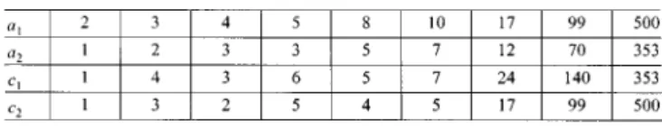
Then, we follow step 4 in Section II-B and assign the values of unknowns to satisfy (28) and (29), shown at the bottom of the next page. We find that there are many possible choices for the values of unknowns . We list some possible choices of the parameters as Table II.
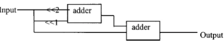
We can implement 8-point ITFT by the method of 1) decimation-in-frequency (as shown in Fig. 2) and 2) deci-mation-in-time (as shown in Fig. 3). We find that both the decimation-in-time implementation and the decimation-in-fre-quency implementation require eight integer multiplications. For the original DFT, we require four real number
TABLE I
SYMMETRY RELATION OF THE 8-POINTS
DFT MATRIX
TABLE II
SOMEPOSSIBLECHOICES OF THEPARAMETERS OF8-POINTSITFT
plications. Although the 8-point ITFT requires twice the multiplication operations and since all the multiplication operations are fixed-point, it will still be more efficient.
From (10), the inverse 8-point ITFT is as in (29), where when
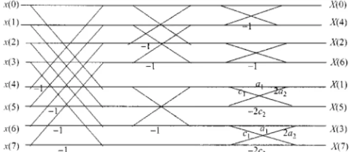
(30) The inverse 8-point ITFT can be implemented as in Fig. 4. We note that the implementation of the inverse ITFT has almost the same structure as the implementation of the forward ITFT in Fig. 2. The difference is that the direction is reverse, and there are some multiplication operations for the input of inverse ITFT. In fact, for all of the the integer transform, the implementations of the forward and inverse transforms will have the same struc-ture.
Fig. 2. Decimation-in-frequency 8-point integer Fourier transform.
Fig. 3. Decimation-in-time 8-point integer Fourier transform.
B. Complete Integer Fourier Transform of 8-Points
After the near-complete integer Fourier transform has been derived, now we will also derive the complete integer Fourier transform. We first discuss the case of 8-points.
We will also use (27) as the prototype of the forward 8-point complete ITFT. In addition, for the inverse transform, we use a similar prototype but modify the parameters as
(27)
Fig. 4. Implementation of the 8-points inverse integer Fourier transform. , shown in (31) at the bottom of the page. There-fore, there are a total of eight parameters. The equality constraint in (28) now becomes
(1) (2) (32)
From the requirement of (12), we also obtain the equality con-straint as
(3)
(4) (33)
where are integer numbers. The inequality constraints in (28) become
(5) (6) (7) (8)
(34) Thus, there are a total of four equality constraints and four in-equality constraints.
To find the values of the eight parameters that satisfy all the above eight constraints directly is time consuming. We introduce a convenient process to assign the values of the parameters as follows. From (1) and (2), we can set
(35) Then, (3) and (4) become
(3 )
(4 ) (36)
We can then implement the following process to find the values of the parameters.
a) Choose the values of such that are integer numbers and
(37) b) Find the integer values of such that
and
where is integer. (38)
c) Set the value of as
is any integer. (39)
Then, the parameters are all obtained.
We list some examples of the parameters as follows. 1)
This is the smallest, simplest integer solution for the pa-rameters. If (40) then . 2) .
We note that when we choose the parameters as the values
list above, the ratios of are all
near to 1.414:1, which is ratio of the original discrete Fourier transform. If is defined as (82), then in this case,
.
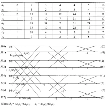
We use Table III to list some possible choices of the values of the parameters of the 8-point ITFT.
We can also implement the forward transform as Fig. 2 or 3 and implement the inverse transform as Fig. 5.
We note that the numbers of multiplication operations required for the 8-point original and complete integer Fourier transform are
Original DFT:
four real numbers, 8 fixed-point multiplication operations Complete ITFT:
20 fixed-points multiplication operations.
TABLE III
SOMEPOSSIBLECHOICES OF THEVALUES OF THEPARAMETERS OF
8-POINTCOMPLETEITFT
Fig. 5. Implementation of the inverse 8-point complete ITFT. That is, we replace four real number multiplication operations with 12 fixed-point multiplication operations. The complete ITFT will be much faster than the original DFT.
C. The Properties and Performance of the 8-Point Complete ITFT
We will see some interesting properties of the 8-point com-plete integer Fourier transform (ITFT). Many properties of the original 8-point DFT will also exist for the 8-point ITFT.
a) Even input even output, odd input odd output: If is even, and is odd
(41) then the complete ITFT of [denoted by ] will also be even, and the complete ITFT of [denoted by
] will also be odd
(42) b) Pure real input conjugated symmetry output, pure
imaginary input conjugated asymmetry output: If is pure real, is pure imaginary, i.e.,
Im Re , and the complete ITFT of
are , then
(43) c) Power preservation property:
If are the complete ITFT of ,
then
where is defined as (40). (44)
d) Time-reverse property and conjugation property: ITFT
ITFT (45)
e) Shift-invariant property:
For the 8-point complete ITFT, if ITFT
(46) then
when is even or when is odd and is even (47)
when is odd and is odd. (48) Equation (47) is satisfied because the equality rela-tions for each row of the original 8-point DFT matrix (listed in Table I) have been kept for the 8-point ITFT; therefore, for the 8-point ITFT matrix, the relation that is still satisfied when is even or when is even. Thus, if the amount of time-shift is even or is even, then
and the relation of (47) has been proved.
Then, we will see the performance of the 8-point ITFT. Here, the parameters we choose are
. Then, we just require 4 bits to implement the kernel of forward ITFT (since the largest entry is ) and require 5 bits to implement the kernel of inverse ITFT (since the largest entry is ).
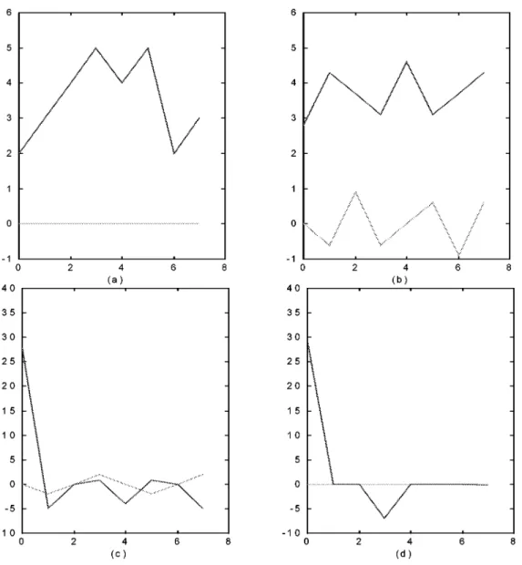
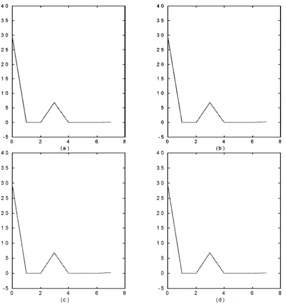
We first see the transform result. We choose two inputs: (49)
(50) We plot them in Fig. 6(a) and (b). (The real part and imaginary part are plotted in separation.). Then, we do the original 8-point DFT, and plot the transform results in Fig. 6(c) and (d). Then, we do the 8-point complete ITFT. To facilitate the comparison, we will normalize the transform results. That is, for the transform result of the complete ITFT
Fig. 6. Transform results of the original, approximated DFTs and complete ITFT. (a), (b) Original signals. (c), (d) Transform results of original DFT. we will normalize by the first column of the forward
integer transform matrix
(52) We plot the normalized transform results of the 8-point complete ITFT in Fig. 7(c) and (d).
We will compare the complete ITFT with the direct approxi-mation of DFT. Since, in this example, we require 4 bits to plement the kernel of forward ITFT and require 5 bits to im-plement the kernel of inverse ITFT, we will also use 4 bits to approximate the forward DFT and use 5 bits to approximate the inverse DFT:
(53)
Here, we use to
de-note DFT, IDFT, approximated DFT, and approximated IDFT, respectively. Then, we use the approximated DFT to calculate
the transform results of and plot the results in Fig. 7(a) and (b).
We then use the following equation to calculate the approxi-mation error.
err (54)
where is the transform result of original DFT. Then, the errors of the four results in Fig. 7 are
for Fig. 7(a): err for Fig. 7(b): err Fig. 7(c): err
for Fig. 7(d): err (55)
We find that the errors are very small. The approximated results of the complete ITFT [Fig. 7(c) and (d)] are even better than the direct approximation (Fig. 7(a), (b)) and are very similar to the transform results for the original 8-point DFT.
Besides, we note that input is the combination of a low-frequency component and a high-low-frequency component. These
Fig. 7. Transform results of the original, approximated DFTs and complete ITFT. (a), (b) Transform results of approximated DFT. (c), (d) Transform results of complete ITFT.
two components can be separated by both original and complete ITFTs. Therefore, the complete ITFT can also be used for the filter design. We can set
is the complete ITFT of when when
to remove the high-frequency component and then do the in-verse complete ITFT for
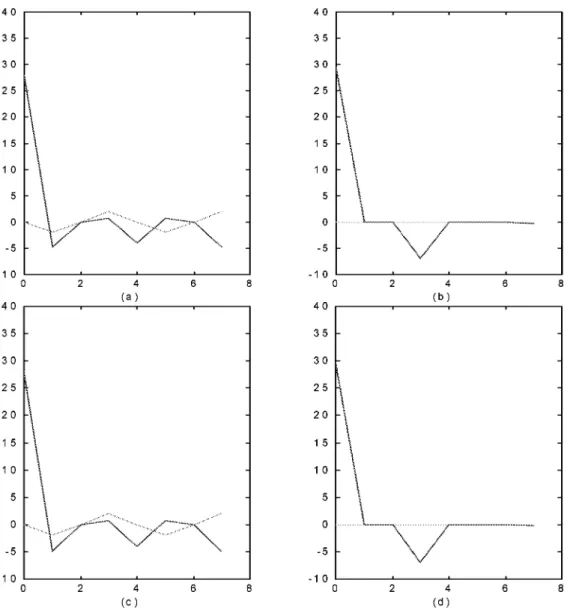
to obtain the filter output. In Fig. 8, we show the filter results. We plot the original signal in Fig. 8(a). Then, we use the original DFT to filter out the high-frequency component, and plot the result in Fig. 8(b). Then, we use the approximated DFT [as (53)] and plot the result in Fig. 8(c). Then, we use the com-plete ITFT and plot the result in Fig. 8(d). Then, we use (54) to calculate the error, but is changed to the filter output by the original DFT, and is changed to the filter outputs
by the approximated DFT and by the complete ITFT. The errors are
for Fig. 8(c): err for Fig. 8(d): err
We find that the error of approximated DFT is about three times the error of the complete ITFT. This is because the complete ITFT is orthogonal and, hence, is reversible. However, the ap-proximated DFT is not orthogonal and reversible, especially when we use fewer bits. Therefore, for the applications that we must do both the forward and inverse transforms, such as the filter design, the performance of complete ITFT will be much better than the approximated DFT.
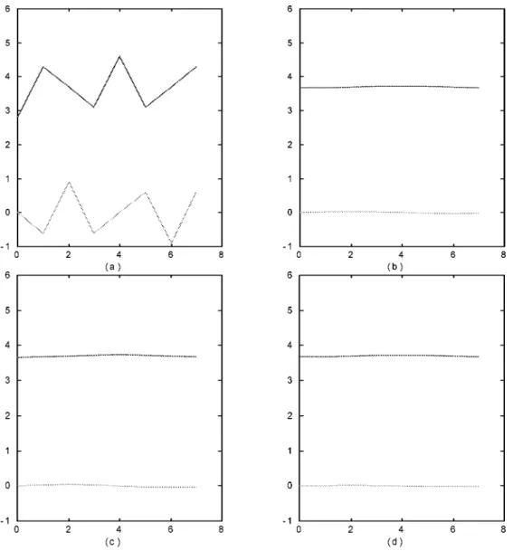
Then, we see the displacement property of the complete ITFT. Here, we use the displacement of input [which is defined in (50)] as the input:
(56) We plot in Fig. 9(a) and (b). Then, we do the complete ITFT for and plot the amplitudes of the normalized re-sults in Fig. 10(c) and (d). We also do the original DFT and the
Fig. 8. Filter experiment. (a) Original signal. (b) Filter by original DFT. (c) Filter by approximated DFT. (d) Filter by complete ITFT.
approximated DFT [as in (53)] for , plot the amplitudes of the results of the original DFT in Fig. 9(a) and (b), and plot the amplitudes of the results of the approximated DFT in Fig. 10(a) and (b).
We find that for the complete ITFT, the displacement property is almost kept. The signal after displacement will have the same transform amplitude as the original signal. When we compare the phase, there is an interesting phenomenon. We find that
angle angle
(57)
angle angle
(58)
This is exactly the same as the original DFT.
Then, we use the equation as below to calculate the dif-ference between (the ITFT or approximated DFT of
) and (the ITFT or approximated DFT of ):
dif or
(59) Then
for Fig. 10(a): dif
for Fig. 10(b): dif (approximated DFT) Fig. 10(c): dif
for Fig. 10(d): dif (complete ITFT) (60) Thus, the complete ITFT will have more excellent displace-ment-invariant property than the approximated DFT, especially when the bits are fewer.
D. Complete Integer Fourier Transform of 6-Points
Because , it seems impossible to avoid the real num-bers multiplication for 6-point DFT, but in fact, we can also de-rive the 6-point complete ITFT.
The original 6-point DFT is
where (61)
By a similar process as the derivation of the 8-point ITFT, we obtain the prototype of the 6-point ITFT as in (62), shown at the bottom of the page. For the prototype as in (92), it is impossible to derive the 6-point complete ITFT; therefore, we modify the prototype a little as in (63) at the bottom of the page. The pro-totype for the inverse transform can be set as in (64), shown at the bottom of the page. From the orthogonality, we obtain the constraints as
(1) (2)
(3) (65)
From the requirement of (12), we obtain the constraints as (4)
(5) (66)
From the inequality relations of the entries of the original 6-point DFT matrix, we obtain the inequality relations as
(6) (7) (67)
Besides, to make (93) and (94) similar to (92), we also impose the following inequality constraints:
(8) (9) (68)
There are a total of five equality constraints and four inequality constraints for ten parameters.
From the constraints 3, 5, we can convert these constraints as
(3 ) (5 ) (69)
and from the constraints 1, 2,
. We can substitute them into the new constraint 5’, and we obtain
(70) Together with constraint 4, we obtain
(71) Thus, to find the values of the parameters, we can follow the process as follows.
1) Choose the value of , and must be satis-fied.
2) Find the value of such that , and where is integer (72)
3) Choose as
where are integer numbers (73) 4) Then, values of can be calculated as
the same as above (74)
(62)
(63)
Fig. 9. Space-invariant property. (a), (b) Shifted input. (c), (d) Amplitude of the transform results of original ITFT.
5) Find the values of such that
are the same as above (75) In addition, the inequality constraints 6 and 7 must be satis-fied.
We give some examples of the values of parameters as fol-lows.
a)
.
This would be the smallest possible choice of the param-eters. If
(76)
then .
b)
.
In this case, the 6-point complete ITFT will be more sim-ilar to the original 6-point DFT. If is defined as (107),
then .
We can implement the forward 6–point complete ITFT as Fig. 11. There are ten integer multiplication operations required. In contrast, to implement the original 6-point DFT, we need eight real multiplication operations. If we consider the overall system, that is, include the forward and inverse transform, then the numbers of multiplication operations required are as
original 6-point DFT:
22 real number multiplication operations.
(eight for forward, eight for inverse, six for normalization) complete 6-point ITFT:
26 fixed-point multiplication operations.
(ten for forward, ten for inverse, six for normalization). It is obvious that the complete integer 6-points DFT is much more efficient.
IV. INTEGERHARTLEYTRANSFORM The discrete Hartley transform (DHT) [5] is defined as
Fig. 10. Space-invariant property. (a), (b) Amplitude of the transform results of approximated DFT. (c), (d) Amplitude of the transform results of complete ITFT.
Fig. 11. Implementation of 6-point integer Fourier transform.
where cas . The transform matrix of the
DHT is just the summation of the real part and imaginary part of DFT
Re Im (78)
The basis vectors of the DHT are orthogonal
The applications of the DHT are similar to the applications of the DFT, and the most important advantage of the DHT is when the input is pure real; then, the output is also pure real.
In this subsection, we will derive the integer Hartley trans-form (ITHT). We will not follow the process introduced in Sec-tion II. Instead, we will just derive the near-complete ITHT as
Re Im (79)
where is the near complete ITFT. We can just derive the complete ITHT as
forward ITHT
Re Im (80)
inverse ITHT
Re Im (81)
where is the forward complete ITFT, and
is the inverse complete ITFT. Here, we have constrained that the ITFT we derive should keep the conjugation system property
(82) The goal of the integer transform is to keep the abilities of the original transform, but no real number multiplication operation is required. If we define the ITHT as (79) or (80) and (81), then the abilities of the DHT will be kept. That is, as the original
DHT, the ITHT defined as (79) or (80) and (81) will be another form of the ITFT, but for the real input, the output will also be real. Therefore, the ITHT may replace the ITFT for processing the real signals.
We then prove that the ITHT is reversible. We prove that the complete ITHT is reversible. From (80) and (81)
Re Re
Im Im
Im Re
Re Im
Since the basis vectors of ITFT are orthogonal, we have
Re Re Im Im Im Re Re Im (83) Thus Re Re Im Im (84) Im Re Re Im (85) and (83) becomes Im Re (86)
Then since, for the ITFT, we have kept the conjugation sym-metry property of (82) so that
Re Re Im Im (87) Re Re Im Im (88) we have Im Re Im Re Im Re Im Re Im Re (89) and (86) becomes (90) From (27) and (79), we can derive the prototype of the trans-form matrix of 8-point near-complete ITHT as (91), shown at the bottom of the page. The constraints are the same as (28).
Similarly to the near-complete ITFT, we can choose the values of as the values listed in Table II.
For the 8-point complete ITHT, the prototype of the forward transform matrix is the same as (91). From (31) and (81), we can derive the prototype of the inverse transform matrix of the 8-point complete ITHT as (92), shown at the bottom of the page.
The values of must also satisfy the
constraints of (32)–(34). We can also choose the values of the as in Table III.
We draw the implementation of the forward, inverse ITHT as Figs. 12 and 13.
For the original DHT and complete ITHT, the multiplication operations we required are
original DHT:
four real number, eight fixed-point multiplication operations complete ITHT:
20 fixed-point multiplication operations.
Although there are fewer multiplication operations for the orig-inal DHT, four of the multiplication operations are real numbers. For the complete ITHT, although there are more fixed-point multiplication operations, there are no real number multiplica-tion operamultiplica-tions. Thus, the complete integer Hartley transform will be simpler and faster.
V. INTEGERSINE ANDCOSINETRANSFORMS
A. Integer Sine Transform of 8-Points
There are many types of DST [6]. In [2], they have derived the 8-point integer: even sine-1, even sine-2, even sine-3, odd sine-1, and odd sine-2 transforms. We describe the 8-point in-teger even sine-1 transform. Others can be seen in [2].
The original 8-point discrete even sine-1 transform is defined as
where (93)
Fig. 12. Implementation of the forward 8-point complete integer Hartley transform.
Fig. 13. Implementation of the inverse 8-point complete integer Hartley transform.
In [2], they have derived the prototype of the 8-point integer even sine-1 transform (ITST-1) as
(94) There are four unknowns . The constraints of the parameters are
(1) (2)
(3) (95)
There are many possible choices of the values of these unknowns (see [2, Tab. II]). One example is (This is the example where the parameters are smallest).
The implementation of the 8-point ITST-1 has not been dis-cussed in the previous works. We draw the implementation of the 8-point ITST-1 as Fig. 14.
The implementation of the 8-point ITST-1 requires a total of eight fixed-point multiplication operations. Since the 8-point ITST-1 introduced above is a near-complete integer transform, there are still eight real number multiplication operations re-quired for the inverse transform. It is very hard to derive the complete integer sine transform.
B. Integer Cosine Transform of 8-Points
In [1], they have derived the integer cosine transform (ITCT), which approximates the 8-point discrete cosine transform
where (96)
The prototype matrix of ITCT is
(97) The constraints are
(1)
(2) (3) (98)
Other details about ITCT can be seen in [1] and [2]. The 8-point ITCT can be implemented as Fig. 15.
In [1], they have also discussed the implementation of the 8-point integer cosine transform. In the above, we use an al-ternative method to implement it, and only the fixed-point mul-tiplication operations are required. As in [1], we set . Here, we try to make the number of multiplication operations as small as possible. If we implement the 8-point ITCT as in Fig. 15, there are 12 integer multiplication operations required for both the forward and inverse transform, but there are still six real number multiplication operations required for the inverse transform.
After the 8-point integer cosine transform (ITCT) defined in (97) has been derived in [1], in [3] and [4], the 16-point ITCT has been derived. In [2], the 8-point integer even cosine-2, odd cosine-1 transforms have been derived, and the ITCT defined as (97) is treated as the 8-point integer even cosine-1 transform.
We can also derive the complete integer cosine transform and do not require any real number multiplication operations, no matter what the forward or inverse transform. We also use (97) as the prototype for the forward ITCT. For the inverse ITCT,
Fig. 14. Implementation of the 8-point ITST-1.
Fig. 15. Implementation of 8-point integer cosine transform.
we also use the same form of prototype, but the parameters are changed as in
(99) Thus, there are a total of 12 parameters
. Then, from the requirement of dual or-thogonality, we obtain the constraints as
(1)
(2) (100)
From the requirement that the inner product must be the value of , we obtain
(3)
(4) (101)
where are integer numbers. We keep the two inequality con-straints in (98) as
(5) (6) (102)
For flexibility, we omit the inequality constraints required for . Thus, we obtain four equality constraints and two inequality constraints.
Although there are 12 parameters and four constraints, it seems that there would be many possible solutions for the
values of the parameters. However, these solutions are hard to find. We introduce a special method to find the solutions. We set , and constraints 1, 2, and 3 become
where is an integer (103) Therefore, we want
det
where is an integer (104) Then, we can assure the solution of will all be the values of the form as , where are integer numbers. We then want
where is an integer (105) The values of that satisfy (105) are hard to find. Therefore, we suppose
i.e., (106)
Then, (38) becomes
where is an integer (107) We further suppose that ; therefore, the requirement becomes
where and must be an integer (108)
Thus, we can do the following process to choose the parameters. a) First, find the value of to satisfy con-straint 4. Since, for the original cosine transform,
, and , we
can choose and and substitute them into constraint 4 to find the values of .
b) Set and , where is an integer number.
c) Choose , and set as
must be an integer (109) d) Calculate from
is an integer (110) e) Check whether . If not, go back to step b). f) Solve from (103).
Then, we can obtain the values of all the parameters. However, we must be careful to satisfy the inequality constraints.
We list some other possible choices of the values of parame-ters as Table IV.
We note that the forward ITCT can be implemented as Fig. 15. The inverse ITCT can also be implemented in Fig. 15, but the direction is reversed with some multiplication operations at the input. There are 12 fixed-point multiplication operations both
TABLE IV
SOMEPOSSIBLECHOICES OF THEVALUES OF THEPARAMETERS OF THE
8-POINTCOMPLETEITCT
Fig. 16. Data structure including the sign, mantissa, and exponent terms. for the forward and inverse transform. There are eight multipli-cation operations for , where is defined as
(111) Four of the multiplications of can be absorbed in the multi-plication operations of the inverse transform; therefore, we need a total of 28 fixed-point multiplication operations for the overall system.
VI. DISCUSSION ABOUT THEINTEGERTRANSFORMS A. Advantages of the Integer Transform over Direct Approximation
In this paper, we use the integer transforms to approximate the noninteger transforms. In fact, we can also approximate the noninteger transform directly. For example, we can use the following data structure, including the mantissa and exponent terms to simulate real number operations by the fixed-point operations numerically [10] as in Fig. 16. In Fig. 16, “ ” is the sign of the number, “Exponent” is the exponent term, and “Significand” is the mantissa term. For example, when we use the above structure to express the real value of , we can first approximate as the form of
is a positive integer number is an integer number (112) Then, we can use “ ” to express the minus sign, use “Exponent ” to express the exponent of 2, and use “Significand ” to express the mantissa term. After using the above data structure, we can use the fixed-point operations to simulate the real number operations.
We may ask what are the advantages of the integer transform over the direct approximation method. We list the advantages below. We will just compare the direct approximation method with the near-complete integer transform.
1) The basis vectors of the integer transform are orthogonal. We note that in Section II-A, we have discussed the four requirements for the integer transform. We note that requirements a)–c) are also necessary for the direct ap-proximation method. The key difference between the in-teger transform and the direct approximation method is requirement d). That is, for the complete integer trans-form, the basis vectors of the forward transform is dual orthogonal to the basis vectors of the inverse transform. However, for the direct approximation method, the basis
vectors of the transform matrix may not be orthogonal. This difference is very important, and many of the advan-tages of the integer transform come from it.
2) The integer transform is reversible, but the transform ob-tained by direct approximation will not be reversible.
Since the complete integer transform is dual orthog-onal, i.e., the basis vectors of the forward transform ma-trix are dual orthogonal to the basis vectors of some matrix , then , where , which is defined as (12) and (14), is the inverse of the forward transform.
However, for the direct approximation method, since the basis vectors are not orthogonal, if the forward trans-form matrix is , then the inverse of (i.e., ) will not be as simple as the inverse of the integer transform. Furthermore, the entries of can usually just be ap-proximated and not explicitly expressed as the data struc-ture as Fig. 16. Thus, although the basis vectors of the original transform (which are denoted by ) are orthog-onal, when we use the data structure as Fig. 16, we will use a transform matrix to approximate and use an-other transform matrix to approximate . Since
(113) we use the data structure as Fig. 16 to approximate a reversible transform; then, the approximated transform would not be reversible.
The reversible property is very important, especially for the applications such as the filter design, data com-pression, and other applications that must do both the for-ward and inverse transforms. Although, for the directly approximation method, if the number of the bits are suffi-cient, then the approximated transform will be almost re-versible. However, for the integer transform, we can use far fewer bits to obtain the reversible transform.
3) The integer transform can use fewer bits to obtain the accurate approximation results.
This is because when we use the data structure as in Fig. 16, some bits must be used for the exponent. Besides, the length of the data structure in Fig. 16 is usually fixed to 16 or 32 bits [10], but for the integer transform, the approximation results are sufficient, even when we use fewer bits. For example, for the two experiments about the ITFT in Section III-C, the largest parameter we choose is , and it only requires 5 bits. Other parameters require 4 bits or less. From the experiment results, we still get accurate approximation results.
4) For the integer transform, when the input is expressed as the fixed-point representation, we do not need to convert it as the real number representation in Fig. 16. We can process it without any real number processor during the overall system.
5) More properties will be kept for the integer transform. For example, the power preservation property will be kept for the complete ITFT (see Section III-C), but this property will not be kept when we approximate the DFT directly.
In conclusion, even when we use fewer bits, the integer trans-forms can still approximate the original transtrans-forms well and re-tain the properties and performance of the original transform. If we use enough bits, then using the direct approximation method will also have the advantages described above. In this case, the advantages of the integer transform may not be so obvious as the case where we use fewer bits.
B. Which Set of Parameters Is the Best
From the discussion about the integer sine, cosine, Hartley, and Fourier transforms, we find that the number of the equality constraints is always less than the number of the parameters. Thus, there are always infinite possible choices for the parame-ters. Thus, we have a question: Among these choices of param-eters, which one is the best? Here, we will discuss this question. To discuss which set of the parameters is the best, we mainly consider two aspects.
1) For the implementation, we want the parameters to be as small as possible. As in Fig. 1, for binary implementation, the entire number is decomposed as
where (114)
Thus, if the parameters we choose are small, then the number of such that will usually be less. Then, for the binary implementation, the number of binary-ad-dition operations and binary-shifting operations will be less.
2) For the performance, we want the ratios of the entries for each row of the integer transform matrix to be approxi-mated to those of the original transform matrix.
For example, for the 8-point ITFT that has the prototype (27), from (15), the original 8-point DFT will have the parameters
as
(115) Therefore, if we want the performance of the 8-point ITFT to be similar to the original, then we want
(116) For the complete integer transform, it is difficult for the param-eters of the forward and inverse transforms to have the ratios approximated to the original at the same time. In this case, the parameters of the forward transform will have higher priority. If the parameters of the forward transform have ratios similar to the original transform, then the transform result will be similar to the original transform.
In [1], the tradeoff between how large the values of unknowns we choose and the performance for the integer cosine transform is discussed. In fact, this tradeoff also exists for other integer transforms. If the unknowns we choose are very large, than it is possible for the integer transforms to better approximate the original transforms and make the performance better; however, the implementation will be tough. On the other hand, if the values of unknown are too small, then the implementation is easier, but the performance is usually worse.
Fig. 17. (a) Implementation of 8-point ITFT (decimation-in-frequency) between the fifth position of the second stage and the fifth and sixth position of the third stage. (b) Binary implementation of Fig. 17(a) whena = 4 and
c = 3. (c) Simplification of (b).
To find the optimal choices for the parameters is hard work. We suggest a way to find the better choices for the parameters.
1) First, find the ratios between the parameters for each row of the original transform matrix.
2) Then, assign the smaller integer values for the parameters such that the ratios are approximated well, and all the constraints for the parameters are satisfied.
Then, although we may not obtain the optimal choices for the parameters, the integer transform we obtain will perform better with simpler implementation.
C. Some Special Methods to Implement Further More Efficient Suppose , where are integer numbers; then if we want to multiply a number , we can first decompose as the linear combination of the powers of 2:
where (117)
For the integer transform, all the multiplication operations can be implemented by the method of (117), and all use the binary shifting and the addition operations. Sometimes, the amount of multiplication operations is huge, or the numbers we want to multiply are very large. In such a case, there will be a lot of binary shifting and addition operations required. We intro-duce some ways to decrease the number of addition and binary shifting operations as follows.
1) Decompose properly so that in (117), the amount of that will be minimum.
For example, we can decompose 15 as
or . However,
the former has 4 s not equal to 0, and the latter only has 2 s not equal to 0. When multiplying 15, decomposing 15 as will require less binary addition operations.
2) Some multiplication operations with the same multipli-cand can be merged together.
For example, for the 8-point ITFT implemented by dec-imation-in-frequency (Fig. 2), between the fifth position of the second stage and the fifth and sixth position of the third stage, there is the branch as Fig. 17(a). For the case
that and , when we implement the
mul-tiplication of 3 and 4 individually, then we must require two binary shifting operations and one addition opera-tion, as in Fig. 17(b). In fact, we can implement these two multiplication operations together. We can decompose 3 as , and then, there is one binary shifting operation that is common for the multiplication of 3 and 4. Therefore, when we implement the multiplication of 3 and 4 together, then one binary shifting is saved, as in Fig. 17(c).
VII. CONCLUSION
In Sections III–V, we only derive the integer cosine, sine, Hartley, and Fourier transform of eight points and the integer Fourier transform of six points. In fact, we can also derive the integer transforms analogous to other noninteger transforms in a similar way.
For the integer transform, we can replace the real number multiplication operations with the fixed-points multiplication operations. Especially for the complete integer transform, there are no real number multiplication operations required. Thus, the integer transform is very efficient. If the datum we want to process are all integer numbers, using the complete integer transform is especially efficient, such as in image and video pro-cessing. This is because during the whole process, there are no real number processors required.
The concept of integer transform analogous to the noninteger transform is very new, and there has been little about it until now. Because they are convenient for implementation and almost re-tain the quality of original noninteger transform; therefore, they can compete with the original discrete transform in many appli-cations. We believe the integer transform will be very popular in the future.
REFERENCES
[1] W. K. Cham, “Development of integer cosine transform by the principles of dyadic symmetry,” Proc. Inst. Elect. Eng., pt. 1, vol. 136, no. 4, pp. 276–282, Aug. 1989.
[2] W. K. Cham and P. P. C. Yip, “Integer sinusoid transforms for image processing,” Int. J. Electron., vol. 70, no. 6, pp. 1015–1030, 1991. [3] W. K. Cham and Y. T. Chan, “An order 16-integer cosine transform,”
IEEE Trans. Signal Processing, vol. 39, pp. 1205–1208, May 1991.
[4] S. N. Koh, S. J. Huang, and H. K. Tang, “Development of order 16-in-teger transforms,” Signal Process., vol. 24, pp. 283–289, Sept. 1991. [5] R. N. Bracewell, The Hartley Transform. New York: Oxford Univ.
Press, 1986.
[6] A. K. Jain, “A sinusoid family of unitary transforms,” IEEE Trans.
Pat-tern Anal. Machine Intel., vol. PAMI-4, pp. 356–365, Oct. 1979.
[7] W. K. Cham, C. S. Choy, W. K. Lam, and S. M. Chiang, “2-D integer cosine transform chip set and its application,” IEEE Trans. Consumer
Electron., vol. 38, pp. 43–47, May 1992.
[8] T. C. J. Pang, C. S. O. Choy, C. F. Chan, and W. K. Cham, “A self-timed ICT chip for image coding,” IEEE Trans. Circuits Syst. Video Technol., vol. 9, no. 6, pp. 856–860, 1999.
[9] W. K. Cham, “Integer sinusoid transform,” Adv. Electron. Phys., vol. 88, pp. 1–61, 1994.
[10] W. Stallings, Computer Organization Architecture, Principle of
Soo-Chang Pei (F’00) was born in Soo-Auo, Taiwan,
R.O.C., in 1949. He received B.S.S.E. degree from National Taiwan University (NTU), Taipei, in 1970 and the M.S.S.E. and Ph.D. degrees from the Univer-sity of California, Santa Barbara, in 1972 and 1975, respectively.
He was an engineering officer with the Chinese Navy Shipyard from 1970 to 1971. From 1971 to 1975, he was a Research Assistant with the University of California, Santa Barbara. He was the Professor and Chairman with the Electrical Engineering Department, Tatung Institute of Technology from 1981 to 1983 and with NTU from 1995 to 1998. Presently, he is a Professor with the Electrical Engineering Department, NTU. His research interests include digital signal processing, image processing, optical information processing, and laser holography.
Dr. Pei received the National Sun Yat Sen Academic Achievement Award in Engineering in 1984, the Distinguished Research Award from the National Sci-ence Council from 1990 to 1998, the Outstanding Electrical Engineering Pro-fessor Award from the Chinese Institute of Electrical Engineering in 1998, and the Academic Achievement Award in Engineering from the Ministry of Educa-tion in 1998. He has been President of the Chinese Image Processing and Pattern Recognition Society in Taiwan from 1996 to 1998 and is a member Eta Kappa Nu and the Optical Society of America.
Jian-Jiun Ding was born in 1973 in Pingdong,
Taiwan, R.O.C. He received both the B.S. and M.S. degree in electrical engineering from National Taiwan University (NTU), Taipei, Taiwan, in 1995 and 1997, respectively. He is currently pursuing the Ph.D. degree under the supervision of Prof. S.-C. Pei with the Department of Electrical Engineering, NTU.
He is currently a Teaching Assistant with NTU. His current research areas include fractional and affine Fourier transforms, other fractional transforms, orthogonal polynomials, integer transforms, quaternion Fourier transforms, pattern recognition, fractals, and filter design.