Network Design Consideration for Distributed Control Systems

Network Design Consideration for Distributed Control Systems

Feng-Li Lian, James Moyne, and Dawn Tilbury

Abstract—This paper discusses the impact of network

architec-ture on control performance in a class of distributed control sys-tems called networked control syssys-tems (NCSs) and provides design considerations related to control quality of performance as well as network quality of service. The integrated network-control system changes the characteristics of time delays between application de-vices. This study first identifies several key components of the time delay through an analysis of network protocols and control dy-namics. The analysis of network and control parameters is used to determine an acceptable working range of sampling periods in an NCS. A network-control simulator and an experimental networked machine tool have been developed to help validate and demonstrate the performance analysis results and identify the special perfor-mance characteristics in an NCS. These perforperfor-mance character-istics are useful guidelines for choosing the network and control parameters when designing an NCS.

Index Terms—Distributed control systems, networked control

systems (NCSs), network transmission delay, processing time delay, sampling time selection.

I. INTRODUCTION

T

HE trend of modern industrial and commercial systems is to integrate computing, communication and control into different levels of factory operations and information pro-cesses [1]. For example, an integrated manufacturing system might include computer-numerically controlled machines, computer-aided design tools, supervisory controllers, and intelligent monitoring devices. The introduction of control network “bus” architectures can improve the efficiency, flexi-bility, and reliability of these integrated applications, reducing installation, reconfiguration, and maintenance time and costs. The change of communication architecture from point-to-point to common-bus, however, introduces different forms of time delay uncertainty between sensors, actuators, and controllers. These time delays come from the time sharing of communi-cation medium as well as additional functionality required for physical signal coding and communication processing. The characteristics of time delays could be constant, bounded, or even random, depending on the network protocols adopted and the chosen hardware. This type of time delay could potentially degrade a system’s performance and possibly cause system instability.

Manuscript received November 30, 2000. Manuscript received in final form October 26, 2001. Recommended by Associate Editor A. Ray. This work was supported in part by the NSF Engineering Research Center for Reconfigurable Machining Systems under Grant EEC95-92125.

F.-L. Lian and D. Tilbury are with the Department of Mechanical Engi-neering, University of Michigan, Ann Arbor, MI 48109-2125 USA (e-mail: [email protected]; [email protected]).

J. Moyne is with the Department of Electrical Engineering and Computer Science, University of Michigan, Ann Arbor, MI 48109-2122 USA (e-mail: [email protected]).

Publisher Item Identifier S 1063-6536(02)01770-0.

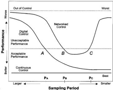
Fig. 1. Performance comparison of continuous control, digital control, and networked control cases.

Research in this class of systems, called networked control systems (NCSs), has focused on two areas: communication protocols and controller design. A proper message transmission protocol is necessary to guarantee the network quality of service (QoS), whereas advanced controller design is desirable to guarantee the control quality of performance (QoP). There are a wide variety of different commercially available control networks such as ControlNet, DeviceNet, Ethernet, Profibus, Sercos, WorldFIP, etc., for the implementation of a NCS architecture. During the NCS design, a performance chart can be derived as shown in Fig. 1. This performance chart provides a clear way to choose the proper sampling period for an NCS. Fig. 1 is the comparison of control performance versus sampling period for continuous control, digital control and net-worked control. The worst, unacceptable, acceptable, and best regions can be defined based on control system specifications such as overshoot, steady-state error, and/or phase margin. The performance axis in Fig. 1 could be chosen to reflect a subset of these metrics. Since the performance of continuous control is not a function of sampling period, the performance index is constant for a fixed control law. For the digital control case, the performance only depends on the sampling period assuming no other uncertainties. The performance degradation point of sampling period in digital control could be estimated based on the relationship between control system bandwidth and sampling rate. For the networked control case, point can be determined by further investigating the characteristics and statistics of network-induced delays and device processing time delays. As the sampling period gets smaller, the network traffic load becomes heavier, the possibility of more contention

time or data loss increases in a bandwidth-limited network and longer time delays result. This situation causes the existence of point in an NCS. The analysis in this paper will show how these points can be computed.

The goals of this paper are to study the key components of time delays and to provide guidelines for obtaining the optimal working range of sampling times. The characteristics of time de-lays are analyzed as a combination of data processing and mes-sage transmission delays; data collected from actual traffic on an industrial control network validates the analysis. The data anal-ysis results provide several time delay models for performance evaluation purposes and the usage of control applications. Based on digital control theory, the impact of sampling period selec-tion is then analyzed. A network-control simulator that takes as input actual device performance profile data, is used to simulate the network traffic with different network protocols, evaluate the control performance of an NCS and validate the phenomena found in the experimental study.

This paper is organized as follows. Section II provides detailed background and related work associated with this study. Section III addresses the key components of time delay between two devices and provides several scenarios to identify these components. Section IV presents the network and control performance analysis in terms of network QoS and control QoP. Section V details the simulation and experimental case study of a networked machine tool. This paper concludes with Section VI.

II. BACKGROUND

There are now a large number of networks available for ap-plications at the information level as well as at the control level. The goal of a control network is to provide a guaranteed quality of service such as deterministic time delays and maximum throughput for real-time control applications. These networks target various types of industrial automation and processing applications and are distinguished through static parameters such as data rate, message size, medium length, supported topology, number of nodes, and dynamic parameters such as medium access control mechanism, message connection type, interoperability, and interchangeability. The detailed compar-ison of these control networks in terms of the above-mentioned parameters can be found in [2]–[4].

Much of the research on the network architecture in con-trol applications has been focused on the network QoS of ex-isting network solutions and then on modifications of the mes-sage scheduling algorithm or medium access control to guar-antee a certain level of network QoS. The network QoS includes predicting time delays, improving throughput, utilization, and efficiency, minimizing lost data rate and calculating message schedulability. Comparisons of network QoS metrics such as network utilization and efficiency versus static network param-eters such as message size and data rate were considered in [6] for several popular control networks. The results provided a first understanding of the NCS time delay without considering other network dynamic parameters which may cause time delay vari-ance. Data latency, or time delay, was analyzed by Ray and Halevi on the medium access control (MAC) mechanism for centralized controlled access, distributed controlled access and

random access [7], [8]. Statistical models of network-induced delays of sensor-controller and controller-actuator links were also studied in terms of message size, period, and station re-sponse time. This statistical information provided a foundation for further analysis of control system stability and performance in a stochastic process setting.

When the time delays do not meet the control system re-quirements, several “traffic smoothers,” for example, were adopted to adjust the message generation rate [9]. These traffic smoothers were installed between the UDP or TCP/IP layer and the MAC layer and gave higher priority to real-time packets over nonreal-time ones. The adaptive traffic smoother harmonically increased and multiplicatively decreased the input limit of real-time or nonreal-time packets to avoid network congestion and improve throughput. Other approaches such as assigning different data sampling periods for different control loops and redesigning network topology into a multihop network were studied by Hong [10] and Tovar et al. [11], respectively. The sampling period of every individual control loop was determined by the limitation of maximum loop delays and the availability of network bandwidth, so as to meet both the control stability con-dition and the network schedulability concon-dition [10]. Multihop topology, on the other hand, provided one quick solution for maintaining the timing requirement [11]. However, additional hardware and software were needed to implement the message transmission between hops, increasing the system cost.

When encountering the degradation of control QoP of an NCS, most studies assumed that, given the information of network-induced delays, robust or optimal controllers could be designed using discrete-time or continuous-time models. Ray et al. used an augmented state to model the network-induced delays within one sampling period and provided design considerations on the stability issues of different time skews and sampling rates in [12] and [13]. Moreover, a stochastic regulator solution that uses dynamic programming and the optimality principle was studied in the presence of randomly time-varying delays [14]. On the other hand, Krtolica et al. expanded the number of states to include the delayed signals, assuming the time delays are equal to multiples of one sampling period [15]. For continuous-time models, studies focused on finding the maximum allowable delay bound based on a Lyapunov stability approach [16]. Based on this bound, they also provided some scheduling algorithms or protocols to guarantee this requirement.

III. TIMINGCOMPONENTS

The important time delays that should be considered in a distributed control system analysis are the sensor to controller and controller to actuator end-to-end delays. In an NCS, message transmission delay can be broken into two parts: device delay and network delay. The device delay1_{includes the time delays at}

the source and destination nodes. The time delay at the source node includes the preprocessing time, and the waiting time, . The time delay at the destination node is only the postprocessing time, . The network time delay includes the

1_{Each device requires processing time for both network communication and}

data acquisition. There may be one processor performing both function or mul-tiple processors. In this paper, we define the total elapsed time required as the pre- or post-processing time.

Fig. 2. A timing diagram showing time spent sending a message from a source node to a destination node.

Fig. 3. Waiting time diagram.

total transmission time of a message and the propagation delay of the network. The total time delay can be expressed by the following equation:

(1) The key components of each time delay are shown in Fig. 2 and will be discussed in the following sections.

A. Preprocessing Time at Source Nodes

The preprocessing time at the source node is the time needed to acquire data from the external environment and encode it into the appropriate network data format. This time depends on the device software and hardware characteristics. In many cases, it may be assumed that the preprocessing time is constant or negligible. However, we will show in Section III-E that this as-sumption is not true in general; in fact, there may be noticeable differences in processing time characteristics between similar devices and these delays may be significant. We will show how experimentally-identified models of the processing time can be used to characterize this delay.

B. Waiting Time at Source Nodes

A message may spend time waiting in the queue at the sender’s buffer and could be blocked from transmitting by other messages on the network. Depending on the amount of data the source node must send and the traffic on the network, the waiting time may be significant. The main factors affecting waiting time are network protocol, message connection type and network traffic load.2_For

example, consider a strobe message connection in Fig. 3. If Slave

2_{In a practical control application, most message transmissions are periodic}

and only the most recent data are used. Hence, in this paper, we do not consider the case where the sender transmits stale messages.

Fig. 4. Nine identical devices with strobed message connection.

1 is sending a message, the other eight devices must wait until the network medium is free. In a CAN3_{-based DeviceNet}4 _network,

it can be expected that Slave 9 will encounter the most waiting time because it has a lower priority on this priority based network. However, in any network, there will be a nontrivial waiting time after a strobe, depending on the number of devices that will re-spond to the strobe.

Fig. 4 shows experimental data of the waiting time of nine identical devices on a DeviceNet network. These devices have a very low variance of processing time. We collected 200 pairs of messages (request and response). Each symbol denotes the mean and the distance between the upper and lower bars equals

3_{CAN stands for controller area network which is a bit-synchronized control}

network that utilizes a nondestructive collision resolution scheme through mes-sage priority specified in the mesmes-sage arbitration field.

4_{DeviceNet implements the physical layer and data link layer of a standard}

CAN protocol and defines its own node and message priority. Specifically, DeviceNet further utilizes the message arbitration field to define different classes of message and node priorities. The waiting time in a DeviceNet network is a function of the message or node number, i.e., priority.

Fig. 5. Processing time histogram of six typical DeviceNet devices.

two standard deviations. If these bars are over the limit (max-imum or min(max-imum), then the value of limit is used instead. It can be seen in Fig. 4 that the average waiting time is propor-tional to the node number (i.e., priority). Also, the first few de-vices have a larger variance than the others, because the variance of processing time occasionally allows a lower-priority device to access the idle network before a higher-priority one. C. Transmission Time on Network Channel

The transmission time is the most deterministic parameter in a network system because it only depends on the data rate, the message size, and the distance between two nodes. The for-mula for transmission time can be described as follows:

, where is the message size in terms of bits, is the bit time and is the propagation time between any two devices. Since the typical transmission speed in a com-munication medium is 2 10 m/s, the propagation time is negligible in a small scale (100 m or shorter) control network. D. Postprocessing Time at Destination Nodes

The postprocessing time at the destination node is the time taken to decode the network data into the physical data format and output to the external environment. Some experimental analysis of postprocessing time along with preprocessing times will be discussed in the following section.

E. Experimental Investigation of Timing Components

In practical applications, it is very difficult to identify each individual timing component discussed above. Instead, by

mon-itoring the time-stamped traffic of the request-response mes-saging on a DeviceNet network, we will show the characteristics of processing times, i.e., the sum of preprocessing and postpro-cessing times of one device.

In the experimental setup, there is only one master and one slave connected to the network and the master continuously polls this slave. Refer to Fig. 2 and let Node A be the master and Node B be the slave. Here, there is no other network traffic other than the request-response messages between the master and slave, i.e., and the request-response frequency is set low enough such that no messages are queued up at the sender buffer. By monitoring the message traffic on the net-work medium and time-stamping each message, we can fur-ther calculate the processing time of each request-response, i.e.,

, after subtracting the transmission time.

Fig. 5 shows the histogram of 400 samples of six typical DeviceNet device processing times. The (right) solid and (left) dashed lines are the maximum and minimum values of pro-cessing times, respectively. The histogram plots indicate the nondeterministic processing times of different network devices and their variance. Devices 1 and 5 have similar functionality of discrete inputs/outputs, but different numbers of input–output modules. Device 5 provides several augmentable modules and hence has more processing units and computation load. Device 1, on the other hand, has only one unit. Devices 2, 3, and 4 have fairly consistent processing times, i.e., low variance. Note that the smallest time that can be recorded is 1 s. The uniform dis-tribution of processing time at Device 6 is due to the fact that it has an internal sampling time which is mismatched with the

(a)

(b)

(c) Fig. 6. Three models of processing time.

request frequency. Hence, the processing time recorded here is the sum of the actual processing time and the waiting time inside the device. Device 6 also provides more complex functionality and has a longer processing time than the others.

In an effort to classify device processing time, we propose three device processing time models as shown in Fig. 6, based on the histograms shown in Fig. 5. The classification of device pro-cessing times is based on a heuristic grouping of experimental data. The first model is similar to the network delay model in [17]. By using these parameters, i.e., s, s, , and , we can specify the probability distribution of the processing time. In model (a), and are the minimum and maximum processing times and is the processing times with higher probability. and are the probability of the two portions. That is

Prob (2)

where . Model (b) is the uniform distri-bution and can expressed by the following form:

Prob (3)

where . Model (c) is the general case; the mul-tiple majority processing times are assumed to have same

prob-ability. Here we classify Devices 1, 2, 3, and 5 as model (a), Device 6 as model (b), and Device 4 as model (c).

IV. NETWORK ANDCONTROLPERFORMANCEANALYSIS

Networks are used to transmit data among control system de-vices. Hence, the network QoS should be analyzed before im-plementing control systems with network architectures. On the other hand, the control QoP should be specified to help evaluate the control system performance. The main evaluation measures of the network QoS are time delay statistics, network efficiency, network utilization, and the number of lost or unsent messages and have been studied in [6]. These measures are used to deter-mine the capability of network medium and provide information to specify control parameters such as sampling period.

A. Control Quality of Performance

In this section we discuss several performance criteria such as IAE/ITAE and control system specifications and their relation to sampling periods. Simulation results relating different time delays and system dynamics are also provided in this section to help provide an understanding of the impact of time delay on control performance.

Two criteria, IAE and ITAE, are generally used to evaluate control system design and performance. IAE is the integral of the absolute value of the error and ITAE is the integral of the time multiplied by the absolute value of the error [18]. Their mathematical formulas are as follows:

IAE or and

ITAE or (4)

where and are the initial and final times of the evaluation period in continuous (discrete) time and is the error between the actual and reference trajectories. ITAE weights later errors heavier and discounts the transient response, whereas IAE weights all errors equally.

When sensors, actuators and controllers are interconnected by one common-bus network, all devices need to share the trans-mission medium. In addition, application signals are discretized. Hence, it is natural to analyze these types of systems using a digital control approach. In order to guarantee system stability and control performance, two control measures can be used to determine the best sampling period: phase margin and control system bandwidth.

The phase margin is the amount by which the phase of an open-loop system exceeds 180 when the magnitude equals one. The primary effect of the sampling time delay is additional phase lag. The phase lags due to discretization, and time delay, , are summarized as follows [19], [20]:

and (5)

where is the system frequency is the sampling period and is the time delay.

The control system bandwidth is defined as the max-imum frequency at which the output of a system will track an

Fig. 7. Impact of time delay mean and variance on control performance.

input sinusoid in a satisfactory manner. In order to guarantee the control QoP, the “rule of thumb” for selecting sampling periods in digital control is that the desired sampling multiple ( ) is [19]:

(6) In order to visualize the impact of sampling and time de-lays on control QoP, a second-order system is considered. Its open-loop transfer function is

(7) The phase margin of this system is 40 at rad/s (as-suming unity feedback). Hence, the maximum sampling period, based on (5), is ms. If considering an additional time delay of 2 ms, the phase lag due to time delay is

using (5). This additional time delay will further reduce the max-imum sampling period.

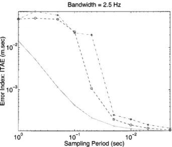
Fig. 7 shows the simulation study of the impact of sampling effect and time delay on control QoP. A closed-loop system with control system bandwidth of 2.5 Hz is studied and the results are shown in Fig. 7. The horizontal axis is sampling period and the vertical axis is ITAE. The (red) solid lines with “ ” are the re-sult of only considering the sampling effect. The (blue) dashed lines with “ ” are the result of considering the sampling effect and a constant time delay of 2 ms. The (green) dashdot lines with “ ” are the result of the sampling effect and a uniformly distributed time delay between 0 and 4 ms. These delays are experienced at both the sensing and actuation nodes. The re-sult of random delay case is the average value of three identical simulation runs. Based on the sampling rule of thumb in (6), the suggested maximum sampling period is 20 ms. For the case without any additional time delay, i.e., only the sampling effect, the control performance gets worse when the sampling periods are larger than the maximum values. When additional time de-lays are also considered, the point of degradation moves to the right. That is, the control performance becomes worse with the

same sampling period. In addition, the case with uniformly dis-tributed time delays shows a further degradation of system per-formance because the time-delay variation causes uncertainty at actuator’s actions.

Fig. 7 demonstrates how point in Fig. 1 can be determined using (5)–(6). If the statistics of the additional time delay are known, point can be determined as follows. Using (5), the total phase lags due to digital control without time delay, and digital control with time delay can be further expressed as follows:

and

(8) Suppose both digital control and digital control with delay have same phase lags, i.e., . Hence, we have

or . Furthermore, (6) can be used to estimate in terms of control system bandwidth, i.e.,

. So, the sampling period of point can be described as follows:

(9) Therefore, using (9) and assuming a 2–ms delay, for the system discussed is estimated as follows:

ms. B. Network Bandwidth Versus Control Performance

For smaller sampling periods, the network traffic is saturated and longer time delays will adversely impact the control perfor-mance. The result of smaller sampling periods and high network traffic load describes the location of point in Fig. 1. There-fore, can be estimated by the total transmission time of all cyclic messages in a control application. However, using

means that the network is saturated. Hence, a better estimation suggested by the sufficient schedulability condition in [25] is as follows:

(10) where 0.69 is the maximum ratio of utilization to meet the suf-ficient schedulability condition for infinite messages.

Further-more, equals for strobe or for poll,

where is the number of devices and is the transmission time of each message. When considering the device processing time, the minimum sampling period, , will increase and can be further modified as follows:

(11) where is the maximum of all device processing time for strobe, or the sum of all device processing times for poll. C. Sampling Period Selection

Due to the interaction of the network and control re-quirements, the selection of the best sampling period is a compromise. Based on the previous analyzes, smaller sam-pling periods guarantee a better control QoP. However, in a bandwidth-limited control network, smaller sampling periods introduce high-frequency communications and may degrade

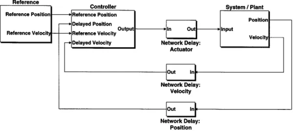
Fig. 8. Simulation model of the networked Robotool in Matlab/Simulink.

the network QoS. The degradation of network QoS could further worsen the control QoP due to longer time delays when network is near saturation. These issues will be further illustrated in the following section by the simulation and experimental study of a networked machine tool.

V. CASESTUDY: A NETWORKEDMACHINETOOL

In this section, we provide a case study of network configura-tion on a machine tool. We investigate the interacconfigura-tion between network and control system parameters through simulation and experiment.

A. System Setup of the Machine Tool

The machine tool studied has three axes: , , and . Each axis moves on a linear slide and is driven through a ball screw by a dc motor with a tachometer, which provides an angular velocity measurement. The dc motor is driven by a PWM drive with control input between zero and 255. Each axis also has a linear encoder that provides linear position measurement. Therefore, both position and velocity feedback are available. The three axes operate independently. The mathematical model of each axis between the PWM input ( ) and the position output ( ) is described by a second-order linear transfer function:

(12) The time constants (s) for each axis are 0.055 ( ), 0.056 ( ) and 0.040 ( ) and the overall gains ((mm/s)/PWM) are 8.346 ( ), 8.956 ( ) and 1.606 ( ), respectively. In the past, several authors used the machine tool as a testbed for research on open architecture control systems [21], supervisory control [22] and cross-coupling control [23]. All previous work used a traditional point-to-point communication architecture. We have installed a DeviceNet network system on the machine tool to study the ad-vantages of a distributed architecture and the impact of network induced delays on control performance.

B. Simulation Model

A network-control simulation model has been implemented in Matlab/Simulink as shown in Fig. 8. The simulation model has two parts: a network simulator and a control simulator. By specifying the MAC mechanism of different protocols and network parameters such as node numbers, data rates, data sizes and message periods, the network simulator produces the network induced delays between different nodes with experimentally determined device performance profiles and provides statistics of these time delays and related network QoS evaluation of the network configuration. Three types of network protocols, Ethernet, ControlNet (token-passing) and DeviceNet (CAN-based) are implemented in the network simulator.5 _The

time delay data can be fed into the control simulator to simulate the dynamic response of the closed-loop system with network induced delays. A PID controller is used on each axis of the machine tool; gains are calculated based on a discrete-time model of the system and a set of desired closed-loop poles. The control simulator also provides the control QoP in terms of ITAE and IAE. The detailed description of this simulation software package can be found in [24].

C. Simulation Study With Network Delay

In this section, we consider the cases with network-induced delays only. Device processing time delay will be discussed in the next section. In this study we consider two fundamental mes-sage connections: strobe and poll. In a strobe connection, all sensors are asked for new information at the same time and the response messages are received by the controller one at a time based on the different network protocols. The controller then calculates the actuation command based on the control law and sends the command to the actuators through the network. For the case of a poll connection, sensors respond with new infor-mation after they have received poll requests. Because sensing messages arrive at the controller at different time instants, it is possible for the controller to update the actuation command im-mediately to obtain better control performance. However, this

5_{The detailed description and comparison of Ethernet, ControlNet, and}

high-frequency updating will generate more network traffic and further increase the time delay. Hence, we only consider the case of a single actuation during each sampling period. Also, if the network is overloaded, the sending nodes only transmit the most current data when the network is available, i.e., stale backlogged data are discarded.

The reference trajectory considered in this simulation study is

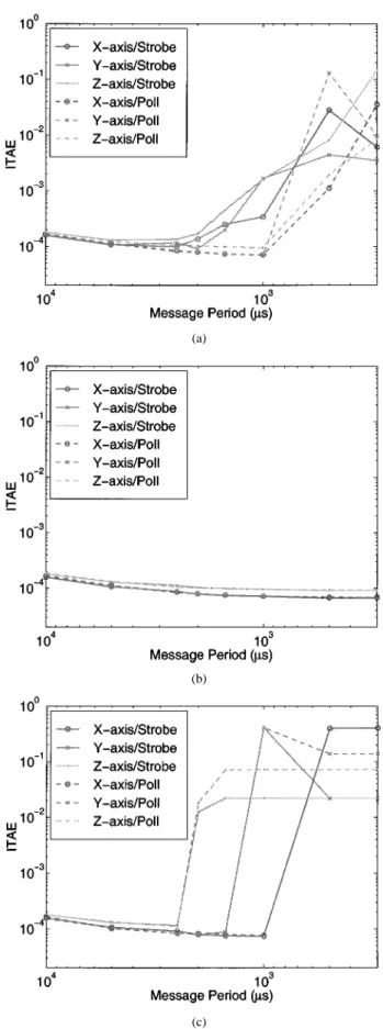
for the and axes, where is the unit step function. The reference trajectory of the axis is equal to half of that of the and axes since the axis has a shorter working range in the experimental setup. ITAE is used to evaluate the control per-formance. The ITAE results, shown in Fig. 9, illustrate the sim-ulated control performance of each axis of the networked ma-chine tool using Ethernet (at 10 Mb/s), ControlNet (at 5 Mb/s), and DeviceNet (at 500 Kb/s), respectively, and strobe and poll message connections. As expected from classical digital control theory, the ITAE value becomes smaller as the sampling rate in-creases and the system performance becomes worse when time delays are longer.

When the time delay varies due to network characteristics, the ITAE values first decrease and then increase as the sampling rate increases. The decrease occurs when the network has a rel-atively low traffic load or is unsaturated; thus, the performance is similar to the constant time delay cases. However, as the sam-pling rate increases, a large number of messages (i.e., higher frequency messages) are contending for the network medium and the time delay of each message becomes larger when total number of messages that need to be sent requires more network bandwidth than available from the transmission medium. There-fore, the ITAE values increase above a critical period. These critical periods are a function of the transmission time to finish transmitting all messages. This is the occurrence of point in Fig. 1. Because the node numbering has little effect in Ethernet and ControlNet, the performance of the three axes are similar in Fig. 9(a) and (b). However, for DeviceNet in Fig. 9(c), the node numbering has a significant effect because nodes are prioritized. In this simulation we set the -axis nodes as high priority and the -axis nodes as low priority, thus the performance of the

-axis subsystem worsens first.

Although we only show the comparison of three different net-work protocols, the simulation tool can be programmed for other network solutions as well. The type of simulation study is useful for the first stage of NCS design where the physical network and control system are not available yet. Hence, by simulating network and control models, an NCS designer can compare the performance and decide on the best network protocol for this specific control application. In addition to the network trans-mission delays, device processing times can also be included in the simulation tool [24].

D. Simulation Study With Network and Device Delays

The simulation study in previous subsection provides infor-mation on how the delays associated with different network pro-tocols impact control performance. However, in practical appli-cations, device delays such as software and hardware processing times are also important as discussed in Section III. In this sec-tion, a set of timestamped network traffic data is collected from

(a)

(b)

(c)

Fig. 9. Control performance (ITAE) versus message period of three control networks and two messaging connections. (a) Ethernet. (b) ControlNet. (c) DeviceNet.

a DeviceNet network. There is one controller node and nine nodes of input–output modules which are used as the interface

Fig. 10. Simulation and experimental results of control QoP: centralized and networked cases. Top row: (a), (b), (c). Bottom row: (d), (e), (f).

between physical sensing/actuating devices and the DeviceNet communication medium. By analyzing the timestamped net-work traffic, the actual time delays between the sensors/actu-ators and controllers can be obtained. These time delays can be further fed into the network-control simulator.

Fig. 10(a)–(c) show the simulation results with actual net-work data. In each plot, the horizontal axis is the sampling pe-riod (s) and the vertical axis is the performance index, i.e., trajec-tory error in terms of ITAE (ms). The (red) dashed lines with “ ” are the results of digital sampling effect only and the (blue) solid lines with “ ” are the results with actual network traffic data which includes network and device delays. In this example, the axis has a higher priority than the and axes. Hence, with smaller sampling periods, the network traffic load is heavy and some of the - or -axis messages do not get through. There-fore, the control performance of and axes degrades first. Note that the and axes have similar dynamic characteris-tics and reference trajectories, but the axis is slightly different, as described in (12). Fig. 10(a)–(c) demonstrate the same time delay effect discussed in Section IV and shown in Fig. 7. How-ever, Fig. 10(a)–(c) also indicate that as the sampling period de-creases, the control performance gets worse when the network load is near saturated. Therefore, in this example, at a sampling period of about 7 ms the axis is still in control, but the and

axes are out of control.

The trend of the simulation result with actual network and device delays here agrees with the DeviceNet case in the pre-vious section, except for the exact sampling periods where the system performance degrades. In the previous section, only net-work transmission time was considered. The simulation sce-nario here includes both network and device delays and the sim-ulation result suggests that the device delays contribute more to the performance degradation than the network delays. Hence, in addition to using a high-speed network and a proper MAC protocol for control applications, networked devices with small processing delays must be chosen.

E. Experimental Study

Fig. 10(d)–(f) illustrate the experimental results of the corre-sponding simulation results shown in Fig. 10(a)–(c). The sam-pling periods considered range from five to 500 ms. The mes-sage transmission is controlled by the polling rate of the master device in a DeviceNet network. Because of the variance in pro-cessing times, the sampling periods are not identical but have a small variance. This further degrades the performance when compared to the digital control case.

The experimental results in Fig. 10(d)–(f) show that the axis has wider feasible range of sampling periods than the and axes because the axis has the highest priority. When

the network traffic load gets heavy, only the messages associated with the -axis can get through. However, all three axes have the same upper limit of sampling period, i.e., ms in the example, since they have similar closed-loop dynamic char-acteristics. The feasible range of sampling periods for the , and axes are (7, 23), (13, 23), and (13, 23) ms, respectively. The results are similar to the simulation results shown in the top row of Fig. 10, although the performance is worse in the cases of longer sampling periods.

VI. CONCLUSION

This paper addressed the design issues of network archi-tecture in a type of distributed control system where sensors, actuators, and controllers are interconnected by a common-bus network. Design considerations include network parameters, control parameters and networked control system performance as the design guideline. Along with the theoretical analysis, a numerical computer network-and-control simulation tool was developed to assist in NCS design. The design procedures are summarized as follows. At the first stage of a design process (assuming actual network and control systems are not available), an NCS designer can utilize the network and control performance analysis in Section IV to investigate the feasibility of this set of system parameters. Also incorporating the pro-cessing time model and other timing parameters described in Section III, an integrated computer network-and-control sim-ulator can be used to help understand the network availability and control performance. Similar comparative analysis can be applied to different network protocols and system dynamics. Hence, the analysis result can be a guideline for choosing the most suitable network system.

If a practical network is available at the next design stage, ac-tual device processing times and network traffic can be collected and used to simulate the control system model. At this stage, different combinations of network parameters can be studied to optimize the control performance. In order to guarantee the best control performance, different controller designs can be tested to verify their stability and performance.

During the design procedure, an NCS performance design chart as shown in Fig. 1 can be derived. This paper investigated the existence and location of the performance degradation points with the aid of simulation and experimental results. The perfor-mance degradation point in digital control can be estimated by using the relationship between control system bandwidth and sampling rate. For the networked control case, point can be determined by further investigating the characteristics and sta-tistics of network-induced delays along with other processing time delays. Messages with smaller sampling periods also gen-erate high network traffic load. The high network traffic load could increase the possibility of data loss or the waiting time for message contention and induce longer time delays. There-fore, network saturation results in the existence of point in networked control.

The improvement of NCS performance can be divided into two areas. One is the minimization of device processing time and the improvement of network protocols to further guarantee

the determinism of transmission time as well as reduce the end-to-end delays. The designer should then pick a sampling period between points and based on other necessary design constraints. The other direction for improvement is advanced optimal or robust controller design which can over-come the uncertainty in an NCS and achieve the best control performance. These improvements can make the performance curve of networked control move toward that of digital control. Our future work will focus on the discrete-time modeling of NCSs which will utilize the network and control parameters identified in this paper. Based on the proposed model, an advanced controller design that consists of both control and network parameters will be implemented to improve the overall NCS performance.

REFERENCES

[1] H. A. Abdullah and C. R. Chatwin, “Distributed C environment for small to medium-sized enterprises,” Integrated Manufacturing Syst., vol. 5, no. 3, pp. 20–28, 1994.

[2] P. Pleinevaux and J.-D. Decotignie, “Time critical communication net-works: Field buses,” IEEE Network, vol. 2, no. 3, pp. 55–63, May 1988. [3] R. S. Raji, “Smart networks for control,” IEEE Spectrum, vol. 31, no. 6,

pp. 49–55, June 1994.

[4] G. Schickhuber and O. McCarthy, “Distributed fieldbus and control net-work systems,” Comput. Contr. Eng., vol. 8, no. 1, pp. 21–32, Feb. 1997. [5] G. Cena, C. Demartini, and A. Valenzano, “On the performances of two popular fieldbuses,” in Proc. IEEE Int. Workshop Factory Commun.

Syst., Oct. 1997, pp. 177–186.

[6] F.-L. Lian, J. R. Moyne, and D. M. Tilbury, “Performance evaluation of control networks: Ethernet, ControlNet and DeviceNet,” IEEE Contr.

Syst. Mag., vol. 21, no. 1, pp. 66–83, Feb. 2001.

[7] A. Ray, “Performance evaluation of medium access control protocols for distributed digital avionics,” ASME J. Dyn. Syst., Measurement, Contr., vol. 109, no. 4, pp. 370–377, Dec. 1987.

[8] Y. Halevi and A. Ray, “Performance analysis of integrated communica-tion and control system networks,” ASME J. Dyn. Syst., Measurement,

Contr., vol. 112, no. 3, pp. 365–371, Sept. 1990.

[9] S.-K. Kweon, K. G. Shin, and G. Workman, “Achieving real-time communication over ethernet with adaptive traffic smoothing,” in Proc.

IEEE Real-Time Tech. Appl. Symp., June 1999, pp. 90–100.

[10] S. H. Hong, “Scheduling algorithm of data sampling times in the inte-grated communication and control systems,” IEEE Trans. Contr. Syst.

Technol., vol. 3, pp. 225–230, June 1995.

[11] E. Tovar, F. Vasques, and A. Burns, “Supporting real-time distributed computer-controlled systems with multihop P-NET networks,” Contr.

Eng. Practice, vol. 7, no. 8, pp. 1015–1025, Aug. 1999.

[12] Y. Halevi and A. Ray, “Integrated communication and control systems: Part I—analysis,” ASME J. Dyn. Syst., Measurement, Contr., vol. 110, no. 4, pp. 367–373, Dec. 1988.

[13] A. Ray and Y. Halevi, “Integrated communication and control systems: Part II—design considerations,” ASME J. Dyn. Syst., Measurement,

Contr., vol. 110, no. 4, pp. 374–381, Dec. 1988.

[14] L.-W. Liou and A. Ray, “A stochastic regulator for integrated communi-cation and control systems: Part I—formulation of control law,” ASME

J. Dyn. Syst., Measurement, Contr., vol. 113, no. 4, pp. 604–611, Dec.

1991.

[15] R. Krtolica, U. Ozguner, H. Chan, H. Goktas, J. Winkelman, and M. Liubakka, “Stability of linear feedback systems with random communi-cation delays,” Int. J. Contr., vol. 59, no. 4, pp. 925–953, Oct. 1994. [16] G. C. Walsh, H. Ye, and L. Bushnell, “Stability analysis of

net-worked control systems,” in Proc. Amer. Contr. Conf., June 1999, pp. 2876–2889.

[17] J. Nilsson, “Real-Time Control Systems With Delays,” Ph.D. disserta-tion, Lund Inst. Technol., Lund, Sweden, 1998.

[18] G. F. Franklin, J. D. Powell, and A. Emami-Naeini, Feedback Control of

Dynamic Systems, 3rd ed. Reading, MA: Addison-Wesley, 1994. [19] G. F. Franklin, J. D. Powell, and M. L. Workman, Digital Control of

[20] M. Malek-Zavarei and M. Jamshidi, Time-Delay Systems: Analysis,

Optimization and Applications. Amsterdam, The Netherlands: North-Holland, 1987.

[21] Y. Koren, Z. J. Pasek, A. G. Ulsoy, and U. Benchetrit, “Real-time open control architectures and system performance,” CIRP Ann., vol. 45, no. 1, pp. 377–380, 1996.

[22] R. G. Landers and A. G. Ulsoy, “Supervisory machining control: Design approach and experiments,” CIRP Ann., vol. 47, no. 1, pp. 301–306, Aug. 1998.

[23] B.-C. Chen, D. M. Tilbury, and A. G. Ulsoy, “Modular control for machine tools: Cross-coupling control with friction compensation,” in

Proc. ASME DSC, vol. DSC-64, Nov. 1998, pp. 455–462.

[24] F.-L. Lian, J. R. Moyne, and D. M. Tilbury, “Networked Control Sys-tems Toolkit: A Simulation Package for Analysis and Design of Control Systems With Network Communications,”, Tech. Rep. UM-ME-01-04, 2001.

[25] C. M. Krishna and K. G. Shin, Real-Time Systems. New York: Mc-Graw-Hill, 1997.