An efficient learning algorithm for function approximation with radial basis function networks

Proceedings of the 9th International Conference on Neural Information Processing (ICONIP'OZ) , Vol. 2 Lip0 Wang, Jagath C. Rajapakse, Kunihiko Fukushima, Soo-Young Lee, and Xin Yao @&tors)

AN EFFICIENT LEARNING ALGORITHM FOR FUNCTION.

APPROXIMATION WITH RADIAL BASIS FUNCTION NETWORKS

Yen-Jen Oyaiig and Shien-Ching Hwang

Department of Computer Science and Information Engineering

National Taiwan University, Taipei, Taiwan

[email protected], [email protected]

ABSTRACT

This paper proposes a novel learning algorithm for constructing function approximators with radial basis function (RBF) networks. In comparison with the existing learning algorithms, the proposed algorithm features lower time complexity for constructing the RBF network and is able to deliver the same level of accuracy. The time taken by the proposed algorithm to construct the RBF network is in the order of O(lSl), where S is the set of training samples. As far as the time complexity for predicting the function values of input vectclrs is concerned, the RBF network constructed with the proposed learning algorithm can complete the task in

O(l7l), where T is the set of input vectors. Another

important feature of the proposed learning algorithm is that the space complexity of the RBF network constructed is O(mlSI), where m is the dimension of the vector space in which the target function is defined. Key terms: Radial basis function network, Function approximation, Machine learning.

1. INTRODUCTION

Function approximation is one of the fundamental issues in machine learning [SI and has been exploited by computer scientists in a number of applications, including data classification and data mining [3]. One widely-used form of function approximators is a linear combination of spherical Gaussian functions as shown in the following:

where cis are the centers of the Gaussian functions, and

IC.

-

cjll is the distance between vector x ant1 ci. Hartman et al. have shown that the linear combination form shown in equation (1) can approximate any function with arbitrarily small error [l].

A function approximator based on equation (1) is generally regarded as a radial basis function (RBF) network. The task of the learning algorithm is to determine the centers, weights, and variances of the Gaussian basis functions. In the original proposal of regularization RBF [ l l ] , the number of basis functions equals the number of training samples. The basis

functions are centered on the training samples and the only unknown parameters are the weights, which can be determined by solving a system of linear equations. However, the resulting networks are complex and often ill-conditioned. Generalized RBF networks are designed with fewer nodes than the number of samples in the training set. As a result, the networks constructed are less complex. The main challenge in such an approach is to determine where the basis functions should be placed and the weights and variances of these basis functions. Several different strategies have been proposed and a good survey can be found in [2]. In recent years, M. Orr proposed a number of alternative learning algorithms for constructing function approximators with RBF networks [6, 7, 8, 91. However, the algorithms proposed by On: suffer high time complexities in the construction of the RBF network, due to the need to compute the inverse of a matrix.

In this paper, an efficient learning algorithm for constructing RBF networks based function approximators is proposed. The time complexity for

constructing a RBF network with the proposed learning algorithm is O(lSl), where S is the set of training samples. As far as the time complexity for predicting the function values of input vectors is concerned, the RBF network constructed can complete the task in O(l7l), where T i s the set of input vectors. Experimental results reveal that the RBF network constructed with the proposed learning algorithm is able to approximate the target function at the same level of accuracy as the RBF networks constructed with the learning algorithms proposed by M. Orr [6, 7, 8, 91. Another important feature of the proposed learning algorithm is that the space complexity of the RBF network constructed is

O(mlSI), where m is the dimension of the vector space in

which the target function is defined.

In the following part of this paper, section 2 elaborates the proposed learning algorithm. Section 3 reports the experiments conducted to evaluate the proposed learning algorithm. Finally, concluding remarks are presented in section 4.

2. THE PROPOSED LEARNING ALGORITHM

The learning algorithm proposed in this paper assumes that samples are taken uniformly over the space of the

function. If the training samples are not exactly located at the crosses of the gridlines, then some sort of interpolation should be conducted. The learning algorithm places one spherical Gaussian function at each training sample and determines the appropriate weights and variances for these Gaussian basis functions. Let f be a function defined in an m-dimensional vector space. Assume that samples are taken uniformly at (bl4 b24..., b,6) over the space of functionf, where bl, bZ,

...,

b, are integers. The learning algorithm presented in this paper will construct a function approximator of the following form:

where

S

is the set of training samples, wi and 0,z are the weight and variance of the Gaussian function centered at sample si, respectively. In the following discussion, it is first assumed that the data set is noiseless. How to deal with noisy data sets will be elaborated later.

Since the influence of a Gaussian function decreases exponentially as the distance increases, when computing the function value at xo based on equation (2), we can include only the Gaussian functions in the proximity of

XO. In other words, we only need to include the

Gaussian functions located within a sphere centered at

XO. The problem now is how large the sphere should

be. In the proposed learning algorithm, the variances of the Gaussian basis functions are uniformly set to a multiple of

S.

Therefore, regardless of where xo is located, the radius of the sphere can be set to a fixed real number determined by the value of

S.

Furthermore, because the training samples are uniformly distributed, we can, in practice, simply include a fixed number of the Gaussian functions centered at the nearest training samples of XO, regardless of where xo is located.

Another assumption that the proposed learning algorithm makes is that the density of training samples is sufficiently high so that the values of function f at the nearby samples of a sample si are all virtually equal to

Asi).

One may argue that this assumption may not hold in real cases. However, the weights of the Gaussian functions determined based on this assumption are just initial guesses. An iterative process will be conducted to fine-tune the weights. Based on this assumption, we can expect that the learning algorithm will set the weights and variances of the Gaussian basis functions centered at si and the nearby samples to virtually the same values. Therefore, the problem of figuring out the weight and variance of the Gaussian basis function centered at si can be modeled by figuring out w i and q

such that

=.f@i)

(3)

where x is a vector in the proximity of si and V I . v 2 ,

...,

v k - 1 are the k

-

1 nearest samples surrounding si.

In order to simplify the subsequent discussion, we assume that function f is shifted so that si is located at the origin. As a result, we can rewrite equation (3) as

Then, we have

because the influence of a Gaussian function decreases exponentially as the distance increases. If we take partial derivatives of g(x1, x2,

. .

.

x

,

)

,

then we will find that

all 1 I j I m. In fact, it can be proved in mathematics that local maximums and local minimums of function g are located at ( ~ 1 4 , UZ&

...,

um4) and

((b,

++)Si,

(b2

++)Si

,

. .

., (b,

+

+)Si)

, respectively, where al, a2,

...,

U, and bl, b2,

...,

b, are integers. Therefore, one approach to make equation (4) above satisfied is to find wi, q such that

We have

g(0,O ,..., 0) = g(*$.k$

)...)

&$) = f ( S i ) . (6)

and

g ( $ 1

+

).

. .

,

+)

To make equation (6) satisfied, we need to set q so that

Let

z

= exp

(

--

.

Then, we can rewrite equation

;2)

-

-

1 + 2 C r ( 2 j ) * = 2 x z ( 2 j + 1 ?

.

(8)

Since 0 <

z

< 1, if we want to find the root of equation

(8), we can take a limited number of terms from both

sides of the equation and find the numerical roots, For

example, if we take the first 5 terms from each si.de of equation (8), then we have

Number of terms taken from each side

of equation (8) 6 (9) Error bound 0.882248 2.8013 x lo-’ root

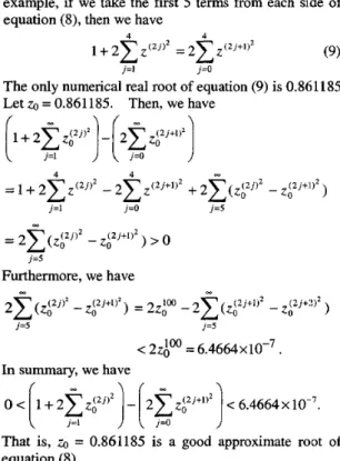
The only numerical real root of equation (9) is 0.861185. Let

a

= 0.861185. Then, we have

1 7 8 9 Furthermore, we have 0.897739 1.2580 x IO+ 0.909615 5.6212 x lo-” 0.919010 2.5010 x lo-’* < 22;” = 6 . 4 6 6 4 ~ 1 0 - ~ . In summary, we have 0 <

[

1

+

2 2

zp)2

-

2 z < 6.4664 x

lo-’

j=l

)

[

j=o

j

That is,

a

= 0.861185 is a good approximate root of equation (8).

In fact, we can find other approximate roots of equation (8) by taking more or less terms from the two sides of the equation. Tab. 1 lists the ,other approximate roots and the corresponding error bounds. As Tab. 1 reveals, if more terms in equation (8) are

included, then the upper bound of error is smaller. However, the magnitude of error is not the only concern for selecting an approximate root. We will address another effect in later discussion.

corresponding error bounds.

Given that

z

= exp

[

-

i-;)

and that

zo

= 0.861185 is a good approximate root of equation (8), we therefore want to set 0;. as follows in order to make equation (7) satisfied:

Equation (10) implies that we want to set the variances

of the Gaussian basis functions in the function

sz

approximator uniformly to -

.

81nk

With the variances of the Gaussian basis functions determined, the next issue to solve is to determine the weights of these Gaussian functions. Based on equation (3), we can derive one equation with each training sample. As a result, if we have n training samples, then we have n equations with n variables, which are the weights of the Gaussian functions. Accordingly, we can solve these equations and find the appropriate weights. However, the time complexity for solving n equations with n variables is very high, exceeding O(n2). Therefore, the empirical approach elaborated in the following is employed in this paper.

Based on equation (6), the empirical approach begins with setting

f

(Si)

w . =

where

p=?=\J&.

Accordingly, the RBF network based function approximator constructed by the learning algorithm is

where 2 = 1

[

+

2 C e x p

I1

- 7 , x is a vector in the

(

i;

11

space o f f , and vl, V Z ,

. .

.

, v k are the k nearest training

samples of x. In fact, when evaluating 2 , we only

need to include a limited number of the exponential terms , because 0 < e 2 < 1 . With

zo

= 0.861185, we have

p=

0.91456 and 2

Fig. 1 uses an example to demonstrate the effect of the learning algorithm based on equation (1 1). As Fig. l(a) shows, the function approximator based on equation (11) deviates from the target function by certain degree around the local minimum and local maximum of the function. The deviation is due to the assumption that the sampling density is sufficiently high. Since the approximate function value computed based on equation (11) is actually a weighted average of the training samples, the smoothing effect shown in Fig. l(a) is expected. As Fig. l(b) shows, if the density of samples is higher, then the deviation is smaller. In this paper, an iterative procedure is developed to compensate the smoothing effect. As shown in Fig. I(c), after the compensation procedure has been conducted, the curve of the function approximator matches that of the target function more accurately. Details of the compensation procedure will be elaborated in the later part of this paper, when noise reduction is addressed.

-2

I . . . . 0 8 - 0 6 - \ , * ,I, >' /-\

-\\m-

7

y;\

0 2 - O -

\\

\>

1

4 6 - \\

/

'\<?

\',

I /

/

'k$ - 0 4 -

i,

0 2 - 1 4 4 -

\h

\\

I

'\$

4

\ - \ iJ,i \ 0 8 - I ,L.,", I , , -2 -15 -1 4 5 0 0 5 1 1 5 -2 -1.5 -1 0.5 0 0.5 1 1.5 2

Fig. l(b). The smoothing effect of the function approximator, when the density of samples is high.

2

i\

o.2

\

4.8 h) i/ 1

?-;.".

1

-2 -1.5 -1 6 . 5 0 0.5 1 1.5 2

Fig. l(c). Effect of the compensation procedure. Now, let us consider another factor to consider in selecting an approximate root of equation (8) from Table

1. If a larger approximate root is selected, then the global variance of the Gaussian basis functions will be larger. As a result, the smoothing effect will be more serious and more iterations in the compensation process need to be conducted.

The discussion so far assumes that the data set is noiseless. In most real-world applications, this ideal assumption does not hold. Therefore, a noise reduction mechanism must be incorporated. In this paper, a naive low-pass filter [ 121 is incorporated at the input of the learning algorithm. Let si be a training sample, and

V I . VZ.

. .

.,

v9 be the q nearest samples surrounding si, and

@si), E(vl),

...,

E(v9) be the random noises associated

with these training samples, respectively. The learning algorithm will use f ( s i ) defined as follows, instead of the observedflsi)

+

E(Si), as the input at sample si:

At the output of the low-pass filter, the variance of noise is reduced by a factor of q

+

1, because

vur[ E ( s ~ ) + E ( v ~ ) + . . . + ~ ( v ~ )

q + l

With the low-pass filter incorporated, the function approximator based on equation (1 1) becomes:

However, the removal of high-frequency components with the low-pass filter is indiscriminate and results in a smoothing effect on the profile of the function. The learning algorithm then resorts to an iterative procedure to compensate the smoothing effect. The compensation procedure will fine-tune the weights of the Gaussian basis functions in equation (1 3) based on the assumption that E[r(t)] = 0 for every training sample

t, where E [ @ ) ] denotes the expected value of random variable E@). According to the law of large numbers in Probability theory, for any real number (> 0, we have

In other words, if r is sufficiently large, then it is highly. likely that E ( S i ) + E ( Y l ) + " ' + E ( V r )

= o

.

Therefore, if

r + l

h i ) z , 3 ( v , >

=

f ( v J 7 h v 2 ) 2 f ( v 2 ) 9 - * e ?

The pseudo-code of the compensation procedure is as follows:

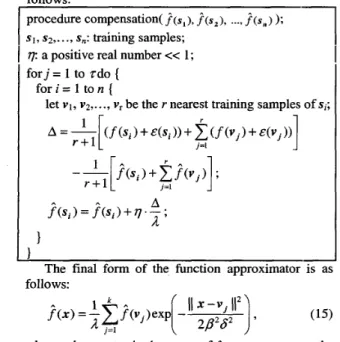
procedure compensation(

?e,),

j(s,), ..., ?(s.) ); SI, sz,

...,

s,: training samples;

q: a positive real number << 1; f o r j = 1 to zdo (

for i = 1 to n (

1

let V I , vz,.

.

.,

v, be the r nearest training samples of 4;

q in equation (1 2) r in equation (14)

zin comDensation Drocedure

I

The final form of the function approximator is as follows:

5

9

5 where x is a vector in the space off, VI. v2,

. .

.,

yk

are the

k nearest training samples of x, and ,8 and

A

are the same constants defined in equation (1 1).

As far as the time complexity of the learning algorithm is concerned, there are four major tasks carried out by the learning algorithm in the construction of a RBF network. The first task is to construct a

hypercube data structure to store the training samples. This task can be done in O(lSl), where S is the set of training samples. The second task is to coinduct low-pass filtering at the input of the function approximator. The time complexity of this task is

O(qlS)), where 4 is number

of

neighboring samples involved in equation (12). The third task :is to construct a function approximator based on equation (13). The only work involved in this task is to determine the values of ,8 and

A

, which can be done in constant time. The last task that the learning algoiithm carries out is executing the compensation procedure. This task can be done in

O(

dSl), where r is the number of neighboring samples in equation (14) and z i s the number of iterations of the outer loop of the compensation procedure. As a result, the overall time complexity of the learning algorithm in the construction of a FU3F network is O(ISI+ qlSl+n$SI). If q, z, and r

are treated

as

constants, then the time complexity is; in a linear order.

With equation (15), the time complexity of' the function approximator for predicting the function values of input vectors is O(k)+O(kIq), where T is the set of input vectors and k is the number of nearest training samples included in equation (15). The term O(k) is due to the time taken to figure out the k nearest training samples of an incoming vector. Because the training samples are evenly spaced, this task can be done in O(k). If k is treated as a constant, then the time complexity is

O(l7l). The space complexity of the RBF network is

O(mISl), where m is the dimension of the vector space in which the target function is defined, because the number of nodes in the hidden layer of the RBF network equals to the number of training samples.

3. EXPERIMENTAL RESULTS

This section reports the experiments conducted to evaluate the proposed learning algorithm. The following three functions are used in the experiments: (i)

(ii)

(Gi) f , ( x l . x z ) = 0.8cos(0.25x1)sin(0.5x2),

The first two functions are 1-dimensional, while the third function is 2-dimensional. The first function is the well-known Hermite polynomial [4]. In each experiment, 100 uniformly distributed samples are taken. A normally distributed random noise with variance = 0.1 is added to each training sample o f 5 andf2, while a normally distributed random noise with variance = 0.03 is added to each training sample of

A.

There is no particular reason why different variances are used, except that it is of interest to observe the impact of different values.

Tab. 2 shows how the parameters of the proposed learning algorithm are set in these experiments. Parameter k is not set, because the number of training samples is not large. As a result, all the basis functions will be included in equation (15). Parameter q is set to 5, because a smaller number does not produce significant effect. A reasonable range of parameter q may be from 5 to 10.

A

value much larger than this

range is not recommended, because the smoothing effect will be more serious. Our experiences suggest that parameter r should be larger than parameter q.

Otherwise, overfitting may occur. The setting of parameter rand

7

are also based on our experience.

The quality of the function approximators is evaluated based on root mean square error ( M S Q defined as follows:

f , ( x ) = 1+ (1-x+ 2x2)e-", x E [-5,51;

f, (x) = e", x E [-4,4];

E [ - 2 , 6 ] , X Z E [ l , 101.

where T i s the set of test samples. In each experiment, the test data set contains 100 randomly selected noiseless samples.

r

Parameter

I

Value

1

I

kin eouation (15) l -

I

77

in compensation procedure

a:

the numerical root of 10.919010

I

0.5

1

equation(8)

Table 2. The parameter setting in the proposed learning algorithm.

In these experiments, the proposed learning algorithm is compared with the three approaches proposed by Orr [6, 7, 91. The three Matlab functions

rbf-fs-2, rbf-rr-2, and rbf-rt-2 that implement Orr's

approaches are available on [lo]. How the parameters and options are set in these modules is listed in Table 3. The list is not exhaustive. For the parameters or options not included in Table 3, the default values were used. The 4 scales used in the experiments are those used in [ 101.

Parameter or option

I

Setting Type of RBF

I

Gaussian

rbf-fs-2 rbf-rr-2

Bayesian information criterion

Model selection criterion

fi

f2

h

0.036+0.008 0.025k0.002 0.09W.022 0.04OH.008 0.021M.002 0.122f0.024

Bias

I

true

Scales

1

[I, 0.5,0.2,0.1]

Table 3. The parameterloption settings in rbf-fs-2, rbf-rr-2, and rbf-rt-2.

rbf-rt-2 proposed

Table 4 shows the RMSEs observed in the experiments. The first number in each entry is the average of 100 independent runs and the second number is the standard deviation. In each of the 100 independent runs, a separate set of training samples is generated. As the numbers in Table 4 show, the proposed learning algorithm delivers the same level of accuracy as the three approaches proposed by Orr in these experiments.

0.045f0.012 0.016f0.003 0.097M.007 0.04W.007 0.016k0.002 0.065f0.005

4. CONCLUSIONS

In this paper, an efficient learning algorithm for constructing function approximators with RBF networks is proposed. The proposed learning algorithm features a linear time complexity for constructing the RBF network. On the other hand, the most well-known existing learning algorithms suffer high time complexity due to the need to compute the inverse of a matrix. Experimental results reveal that the RBF network constructed with the proposed learning algorithm is able to approximate the target function at the same level of accuracy as the RBF networks constructed with the existing learning algorithms. As far as the time complexity for predicting the function values of input vectors is concerned, the RBF network constructed with. the proposed learning algorithm can complete the task in

@)U),

where T is the set of input vectors. Another important feature of the proposed learning algorithm is that the space complexity of the RBF network

constructed is O(mlSl), where m is the dimension of the vector space in which the target function is defined.

Several issues deserve further 'studies. The first issue is data reduction. The current version of the proposed learning algorithm places one basis function at each training sample. It is of interest to develop some kind of data reduction mechanisms to reduce the complexity of the RBF network constructed. The second issue concerns noise reduction. In this paper,

an empirical approach is incorporated. Since noise handling is a critical and challenging issue, further studies are highly desirable. The third issue is the general characteristics of the proposed learning algorithm. More comprehensive experiments should be conducted to learn more about its general characteristics.

5. REFERENCES

[ l ] E. J. Hartman, J. D. Keeler, and J. M. Kowalski, "Layered neural networks with Gaussian hidden units as universal approximations," Neural Computation, vol. 2, no. 2, pp. 210-215, 1990.

S. Haykin, "Neural networks: A comprehensive

foundation," New York McMillan, 1994.

V. Kecman, Learning and Soft Computing: Support Vector Machines, Neural Networks, and Fuuy Logic Models, The MIT Press, Cambridge, Massachusetts, London, England, 2001.

[4] D. J. C. Mackay, "Bayesian interpolation," Neural Computation, vol. 4, no. 3, pp. 415-447, 1992.

[SI T. Mitchell, Machine Learning, McGraw-Hill, 1997.

[6] M. J. L. Orr, "Regularisation in the selection of

radial basis function centres," Neural Computation, vol. 7, no. 3, pp. 606-623, 1995.

M. J. L. OK, "Introduction to radial basis function

networks," Technical report, Center for Cognitive Science, University of Edinburgh, 1996.

M. J. L. Orr, "Optimising the widths of radial basis functions," Proceedings of the Fifth Brazilian Symposium on Neural Networks, 1998.

[9] M. J. L.

Orr,

"Recent advances in radial basis function networks," Technical report, Center for Cognitive Science, University of Edinburgh, 1999. [lo] M. J. L. Orr, "Matlab functions for radial basis

function networks," http://www.anc.ed.ac.uk/-mjol

software1rbf.zip.

[ l l ] T. Poggio and F. Girosi, "Networks for approximation and learning,'' IEEE Proceedings, vol. 78, no. 9,pp. 1481-1497,1990.

[12] L. R. Rabiner and B. Gold, Theory and Application of Digital Signal Processing, Prentice-Hall, Englewood Cliffs, New Jersey, 1974.

[2] [3]

[7]