C.Y. Liou*, W.P. Tai
Department of Computer Science and Information Engineering, National Taiwan University, 10764 Taipei, Taiwan, Republic of China
Received 20 March 1998; received in revised form 30 March 1999; accepted 30 March 1999
Abstract
The self-organization model with a conformal-mapping adaptation is studied in this work. This model is designed to provide conformal transformation to meet the conformality requirement in biological morphology and geometrical surface mapping. This model spans the network field in the input space where topological conformality is preserved. The converged network provides not only the organized clustering features of the input but also a specific mapping representation. This facilitates the Kohonen’s self-organization model in exploring the input in a continuous conformality sense. Simulations for morphing applications are described.q 1999 Elsevier Science Ltd. All rights reserved.
Keywords: Self-organization; Feature map; Conformal mapping; Schwarz–Christoffel transformation; Simplex quantization; Morphological form; Facial
modeling; Neural networks
1. Introduction
The self-organization model (SOM, Kohonen, 1982) is used to organize topologically sensory inputs into clusters on a feature map. An ordered map can provide a coordinated lattice representation for the input space, i.e. the discrete mapping function from the inputs to the network field. This mapping approximates the input space using finite synaptic weight vectors as the clustering centers. This discretized representation may not characterize completely inputs which have continuous structured features. This limits its application in vector quantization tasks.
Continuous mapping has been studied recently with vary-ing success. A continuous model was proposed by Li, Gasteigner, and Zupan (1993) based on concepts of topol-ogy theory. This model provides a method to measure the topology distortion on a feature map. A parameterized self-organizing map algorithm has been proposed by Ritter (1993) for learning tasks in robotics and vision. This algo-rithm constructs an interpolated smooth manifold to approx-imate the input space continuously. There is no specific mapping function in their work.
We attempt to construct a continuous mapping which is in accordance with the intrinsic property of the SOM. During the training process, an approximately conformal transfor-mation can be observed (Tanaka, 1994) in the development
of the network field. The trained network can be regarded as a conformal transformation of the input space (Tanaka, 1994). This property has not been further pursued before and not included in current continuous versions of the SOM model. This inspires us to construct a continuous SOM with exact conformality.
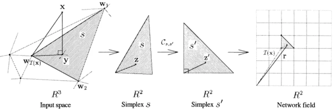
In our proposed conformal SOM (CSM), an explicit continuous space-dependent mapping function between the input space and the network field is derived (see Fig. 1). The whole continuous representation is composed of a collection of local conformal mappings.
Dimensionality reduction from the input space to the network field is also accomplished by this model. The distortion errors in this continuous representation, caused by dimensionality reduction, will be also smaller than those in the quantized representation.
In many practical tasks, for example, biological morphol-ogy (Thompson, 1917) and geometrical surface mapping, continuous conformal mappings are required. Current continuous models (Li et al., 1993; Ritter, 1993) do not satisfy this requirement. The proposed model meets this requirement and helps the SOM accomplish these tasks. These tasks necessitate the use of this network and distin-guish it from other continuous versions of the SOM model. To show the contribution of the model, we will describe applications in morphing and in geometrical surface design. We will briefly review the discrete SOM with notations in Section 2. The simplicial representation is employed to configure the network field (Lemmon, 1994). Section 3 contains the proposed CSM. In Section 4, we describe 0893-6080/99/$ - see front matterq 1999 Elsevier Science Ltd. All rights reserved.
PII: S 0 8 9 3 - 6 0 8 0 ( 9 9 ) 0 0 0 3 4 - 9
* Corresponding author. Tel.:23625336, ext.:515; fax: 1886-2-23628167.
techniques for deriving the mapping functions in two- and one-dimensional space. The algorithm is also summarized. Applications in biological morphology and geometrical surface design are presented in Section 5. Finally, the results are given in Section 6.
2. Review of the self-organization model
The SOM can be described as a process with a best-matching function, I, and a synapse adaptation function, U. The best-matching function I defines the mapping from input set X# Rpto a finite discrete set I in the network field. Each neuron is indexed by a q-dimensional label i [ I, where q is smaller than p usually. Let wi[ R
p
denote the synaptic weight vector of the neuron with index vector i. For a sampled input vector x, the function I decides the best-matching neuron,
I x arg min
j[I
ix 2 wji: 1
Then, the function U adjusts the synaptic weights of neurons with varying updating,
U wi old w i new w i old1a ·h iI x 2 ii·x 2 wi old; i[ I; 2 wherea is a learning rate and h(·) is a neighborhood func-tion. After the training, an ordered representation can be obtained on the map.
Although different discrete metric systems can be used in the network field, the regular grid coordinate system in Rq with the Euclidian distance is commonly used for the metric of I. Using this regular system, the topology and the statis-tics of the inputs can be appropriately preserved on the map. Quantized dimensionality reduction can be obtained in the mapping from Rpto Rqusing the SOM.
To formulate the dimensionality reduction of the input space, a simplicial representation (Lemmon, 1994) of the network is employed. In a network field, each neuron is associated with a collection of neighboring simplices. For a simplex in the network, the corresponding synaptic weights in the input space also form a simplex, as shown
in Fig. 2. Each simplex in Rp is q-dimensional. Let w1, w2,…, and wqbe the synaptic weights of all q neighboring
neurons associated with the neuron having synaptic weight vector wi. Each simplex is defined as the set of all points w of Rpsuch that
w wi1
Xq j1
aj wj2 wi; 3
where 0# ajfor all j and Pq
j1aj# 1 (Munkres, 1984). In
the CSM, the sampled inputs can be mapped to these q-dimensional simplices.
Consider a q-dimensional simplex s in the input space. The simplex s is always a convex polyhedron with q1 1 boundaries, which are (q2 1)-dimensional simplices in Rp.
Let <j1…q112sj; 2sj# s; denote the boundary set of this
simplex s. Each element2sjin the boundary set is a (q2
1)-dimensional simplex. The polyhedral boundaries,<j2sjwill be used to derive the conformal transformation of this simplex by means of the boundary value method.
During the self-organization process, each simplex configuration is reformed following synapse adaptation. A conformal mapping can be formulated for each simplex. We may apply multi-dimensional conformal analysis to construct the mapping function. Let the mapping from simplex s to a corresponding simplex s0be Cs, s0, where C
is defined in Rq, i.e.C: z 7! z0, and z, z0[ Rq.
Usually, the explicit forms for arbitrary conformal mapping functions are difficult to obtain. Numerical techniques must be applied to obtain the mapping. In Section 4, the numerical Fig. 1. The mappingM(x).
conformal mapping for the two- and one-dimensional simplex will be explicitly constructed with such techniques.
3. The conformal self-organization model
Based on this simplicial representation, we can include the conformal property in the self-organization process. The best-matching functionM and the synapse adaptation
func-tionW in the process will be modified. The continuity on
the feature map and the distance measure for M will be discussed.
3.1. Continuity on the feature map
In the CSM, the functionM transforms an input into its continuous reference in the network field. The reference in the network is not restricted to the element in a finite discrete set I; i.e. the network field is continuous so as to represent the input space without discretized quantization.
The topology formed by spanning the network field in the input space can be regarded as a collection of q-dimensional simplices. A sampled input x[ X will be mapped to a best-matching projection vector in one of these simplices. Let the mapped simplex and the best-matching projection in this simplex be s and y, respectively, where y[ s. The simplex
s can be chosen from SI(x), the set of all neighboring simplices of the winning neuronI(x) by Eq. (1).
The simplex on which the input is projected can be found as follows:
s arg min
t[SI x
D x; t: 4
The functionD(x, t) which measures the distance between the input x and the simplex t will be discussed later.
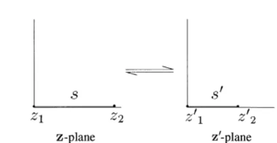
When the projection y for the input x is found, the relative reference z[ Rqin the simplex s, where the point wI(x)is the origin of the Rqplane, is also determined. To obtain the representation of x, this relative reference z will be mapped to the z0 Cs;s0 z in the transformed simplex s0, which has the same configuration as the simplex in the network field. The detailed mapping techniques for the conformal mappingCs,s0from the simplex s to the simplex s0 will be
presented in Section 4. The final reference r I(x) 1 z0in the network field, a grid coordinate in Rqis the representa-tion of the input x. This reference vector r is continuous in the space Rq. Fig. 3 shows all the mappings from the input x to the reference r.
In the CSM, the best-matching function is composed of the above discussed mappings. Let M denote the best-matching function in the model, where M : x 7! r; x [
Rpand r[ Rq. This functionM will conformally transform the input into its continuous representation in the network field. The continuous field can be used to approximate the input space without quantization errors.
3.2. The distance measure
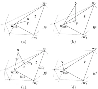
The function D(x, t) in Eq. (4) measures the distance between the input x and the simplex t, t[ SI x. To eval-uate the distance D(x, t), we determine a point y in the simplex t which is nearest to the input x; i.e. the distance from x to this point is shortest among the set t. This distance isix 2 yi.
If an input x[ t, its projection y will be the point x and D(x, t) 0. In other cases, the location of y can be deter-mined using the following procedure. We first evaluate the orthogonal projection of x on the subspace where the simplex t is located. For an input x, its orthogonal projection on this q-dimensional subspace can be determined by
wk2 wI x·x 2
Xq j1
bj wj2 wI x 0; k 1…q;
5 where wj, j 1…q, are the synaptic weights of all q
neigh-boring neurons associated with the simplex t. After solving the variables bj, j 1…q, in Eq. (5), we can test whether the
projection of x is inside the simplex t or not. When the condition in Eq. (3) i.e. bj$ 0 for all j and
Pq
j1bj# 1, is satisfied, this projection is inside the simplex t. The vector y will be
yX
q
j1
bj wj2 wI x: 6
If the orthogonal projection is not located inside the simplex
t, y can be recursively determined from the boundary set
<j2tj by means of successive projections. Note that each
boundary2tj; j 1…q 1 1, is also a simplex of dimension
(q2 1). This procedure (5) and (6) can be recursively used
to find a projection y in one of2tj.
Fig. 4 shows different cases in which the projection points can be determined using the procedure. Since q 2 in most applications, we will limit our discussion to two-dimen-sional cases to clearly demonstrate the procedure.
The minimum projection y in one of the neighboring simplices associated with the neuron I(x) can be found by Eqs. (4) and (6) as the best-matching projection of the input x. In contrast with the SOM, this representation is not limited to the synaptic weight vector wI(x); i.e. there will be no quantization errors. In Section 5, we will demonstrate that the distortion errors of the CSM will usually be smaller than those in the quantized feature map.
3.3. Adaptation with continuous neighborhood function
In the SOM, the processU adjusts the synaptic weights so that they approach the input. Each adjustment is propor-tional to the product of a learning rate and a value of the neighborhood function. The typical neighborhood function is usually a continuous function of the distance in the network field (Kohonen, 1993). Because of discretized indexing in the network field, the neighborhood function always has several fixed output values as shown in Fig. 5. For different inputs which are mapped to the same best-matching neuron, the updates are the same for all corre-sponding synaptic weights. This will have a smoothing effect on the map.
With a continuous feature map, the adaptation process will be more sophisticated in approximating the input space. Let W denote the adaptation function in the CSM. The neighborhood function, denoted by h(d), d[ R, can be defined as a continuous function of the distance between the references in the network field. The distance metric can be simply defined as the Euclidean distance in Rq. For an input
x, the functionW adjusts the synaptic weight vector wifor all i[ I based on the adaptation rule,
W wiold winew wiold1a·h iM x 2 ii·x 2 wiold;
i[ I: 7
Compared with Eq. (2), the vectorM(x) is not a discretized index vector in the network field. The distanceiM(x) 2 ii is continuous in R. Hence, the output of h is also continuous as shown in Fig. 5.
The functionW has the same computational costs as the functionU has. The feature maps trained by these two func-tions may have different maps. Due to the smoothing effect, U may not appropriately adapt the synaptic weights for every kind of input. We will display this using simulations.
4. Numerical construction
We will now discuss techniques for the conformal mappingCs,s0in this model. We will apply numerical
tech-niques (Trefethen, 1980) in the complex domain to solve this boundary value problem. These techniques can solve two-dimensional mappings. We will show how these mappings can be obtained in two- and one-dimensional space.
The mapping functionCs,s0, which transforms the region
from the simplex s to the simplex s0in the two-dimensional network field, can be formulated as a conformal function in the complex plane. Because each simplex in the two-dimensional network is a triangle, the Schwarz–Christoffel transformation (see for example, Henrici, 1974) can be used to construct such a function. By using two Schwarz– Christoffel transformations, a one-to-one mapping between two simplices can be obtained.
Fig. 4. Four different cases for the projection y. (a) The input x is inside the simplex t; (b) The projection inside the simplex t; (c) y is on the boundary 2t1; (d) y is on the vertex wI(x).
Consider the simplex s with vertices labeled zj; 1 # zj#
3; in the complex plane, z-plane, and the simplex s0 with
vertices labeled z0j; j 1; …; 3; in the z0-plane. Using the Schwarz–Christoffel transformation, we can transform the boundary of s along with the vertices into the outer circle of a unit disk in the v-plane and then transform the circle into the boundary of s0. The unit disk in the v-plane is utilized as an intermediate set to assist the Schwarz–Christoffel trans-formation. Fig. 6 shows the mappings between simplices in the complex planes.
First, we will consider conformal mappings from the unit disk in the v-plane to the simplices in the z-plane and z0 -plane. Letbjp; 21 #bj, 1; be the exterior angle of the simplex s at zj and let gjp; 21 #gj, 1; be that of the simplex s0at z0j. For triangles, we have simple relationships
betweenbjp andgjp, respectively, X3 j1 bj 2 and X3 j1 gj 2: 8
The Schwarz–Christoffel formula defines the mapping from
v to z as z zc1 C1 Z v 0 Y3 j1 12 v 0 vj !2bj dv0 9
and the mapping from v to z0as
z0 z0c1 C2 Zv 0 Y3 j1 12 v 0 vj !2gj dv0; 10
where vj, j 1…3, are the points on the circle of the unit
disk in the v-plane which correspond to the vertices of the two simplices and C1, C2, zc, and z0care the complex
para-meters of the mappings. In our model, vj, j 1…3, are
chosen so as to equally divide the unit circle for the sake of accuracy in the numerical evaluation.
The parameters in Eqs. (9) and (10)) are determined as follows. To transform the corresponding points on the boundaries in different planes, the mappings satisfy the complex conditions, zk2 zc C1 Zvk 0 Y3 j1 12 v 0 vj !2bj dv0; k 1…3 11
from v1, v2, and v3to z1, z2, and z3, respectively, and
z0k2 z0c C2 Zvk 0 Y3 j1 12 v 0 vj !2gj dv0; k 1…3 12
from v1, v2, and v3 to z01, z02, and z03, respectively. The
integration in each condition is evaluated by means of the compound Gauss quadrature (see, for example, Davis & Rabinowitz, 1984). The parameters can be estimated from the numerical solutions of Eqs. (11) and (12).
Next, we will consider the inverse conformal mappings from the simplices in the z-plane and z0-plane to the unit disk in the v-plane. The inverse mappings can also be solved by means of numerical methods. By inverting the Schwarz– Christoffel formulas (9) and (10), we obtain
dv dz 1 C1 Y3 j1 12 v vj !1bj 13 for the mapping from z to v and
dv dz0 1 C2 Y3 j1 12 v vj !1gj 14 for the mapping from z0 to v. Numerical o.d.e. algorithms can be applied to solve these boundary value problems. Valid solutions can be obtained through iterative evaluation (Trefethen, 1980).
Because the mapping functionCs,s0is solved using
numer-ical techniques, this CSM requires more computational effort than does the SOM. To reduce the amount of compu-tation, we will consider an approximated solution for the mapping functionC. Suppose that the changes of the exter-ior angles from the simplex s to the simplex s0are small. Let the exterior angles of the simplices s and s0bebjp and (bj1
dj)p, respectively, where j 1…3, udju p 1, and
P3
j1dj 0. Then the integrand in Eq. (12) will be
Y3 j1 12 v 0 vj !2 bj1dj Y 3 j1 12 v 0 vj !2bj ·Y 3 j1 12 v 0 vj !2dj <Y3 j1 12 v 0 vj !2bj ·1 15 Fig. 6. The mappings between simplices in the z, v, and z0planes.
when v0is not the singularities vj, j 1…3. With Eq. (15),
we have
z0< z0c1 C2· z 2 zc=C1: 16
From experience, we know that approximation in Eq. (16) is applicable to cases where 2 0.2p ,dj , 0.2p, j 1…3.
In addition, the closeruv0u is to zero, the center of the unit disk, in the v-plane, the more accurate this approximation is. We will use this approximation in all our simulations in the final relaxation stage. The computations for the conformal mappings are listed in Table 1.
For a one-dimensional network field, the region of each simplex can be regarded as a line segment on the real axis in the complex plane. As shown in Fig. 7, the conformal mapping of the region from the simplex s in the z-plane to the simplex s0in the z0-plane can be defined by
z0 C3z; 17
where C3is the parameter of the mapping. The value of C3
can be determined as the real constant which scales the length of the segment.
Numerical evaluation of the mapping function Cs,s0
requires computation in the training process. From experi-ence, we know that we can employ a modified process to reduce the amount of computation. Before the distortion errors converge, the training results obtained by this model can be shown to be similar to those obtained by the SOM. This will be shown through many simulations in a later section. Therefore, the discrete indexed network can be used until there are no noticeable changes in the distortion errors. The CSM can be used to fine tune the network during the final relaxation stage.
For clarity, we will summarize the algorithm of the CSM. There are iterative training steps in the algorithm to adapt the synaptic weights in order to approximate the input. 1. Give an input set X. Initialize the synaptic weight vectors
wi, i[ I, with random values. The training parameters,
including the total number of adaptation iterationstmax,
the neighborhood function h(d), and the learning rate
a(t) at iteration t, are defined according to the needs of the application.
2. Fort 1,2,…,tmax
(a) Sample a random vector x[ X. (b) Find the best-matching functionM(x). i. Find the best-matching neuronI(x) by Eq. (1). ii. For each simplex t in SI(x), the set of all neighboring simplices of the winning neuron I(x), compute the best-matching projection y in each simplex t. The procedure is recursive for y by Eqs. (5) and (6). iii. The best-matching simplex s is set to be the simplex
t[ SI(x)with a minimum y as Eq. (4).
iv. Determine the relative reference z in the simplex, s. Compute z0 Cs,s0(z) in the simplex s0which has the
same configuration as the simplex in the network field. The conformal transformationCs,s0is constructed using
numerical method.
v. Compute the reference r in the network field by means of r I(x) 1 z0.
(c) The synapse adaptation function W adjusts the synaptic weight vector wifor all i[ I by Eq. (7). (d) Update the learning rate a and the neighborhood function h(d). Continue with the nextt.
5. Simulations and discussion
The distortion of the representation comes from two sources: dimensionality reduction errors and quantization errors. In the CSM, quantization errors can be reduced as in other continuous models (Li et al., 1993; Ritter, 1993). This continuous representation can also be used to approx-imate the input space effectively. To demonstrate its perfor-mance, we will give simulations with different input distributions. We will also test the SOM with the same inputs. We will use this CSM in form transformation for biological development or growth, where conformality in the morphology is required. Other applications such as designing surface shapes in fluid dynamics and cartography will also be included.
5.1. Comparison between the CSM and the SOM
For comparison, we employed both one-dimensional networks with N neurons and two-dimensional networks Table 1
Variables, equations and techniques in the numerical construction of two-dimensional conformal mappings. The execution times of each numerical evaluation during the synapse adaptation process withtmaxiterations are included
Computation Symbol Equations Technique Times
Mapping parameters C1and zc (11) and (8) Compound gauss quadrature tmax
Mapping parameters C2and z0c (12) and (8) Compound gauss quadrature 1
Approximated mapping z0 16 Complex addition and multiplication tmax
with N× N neurons to approximate different input sets in two- and three-dimensional space. The total number of adaptation iterationstmax, the neighborhood function h(d),
and the learning ratea(t) at iterationt is the same in both models. In our simulations, we set tmax 5000,
a t 0:001t=tmax, and h(d) exp( 2 d2/2aN2). The initial network configurations were regularly arranged in the input space for each case.
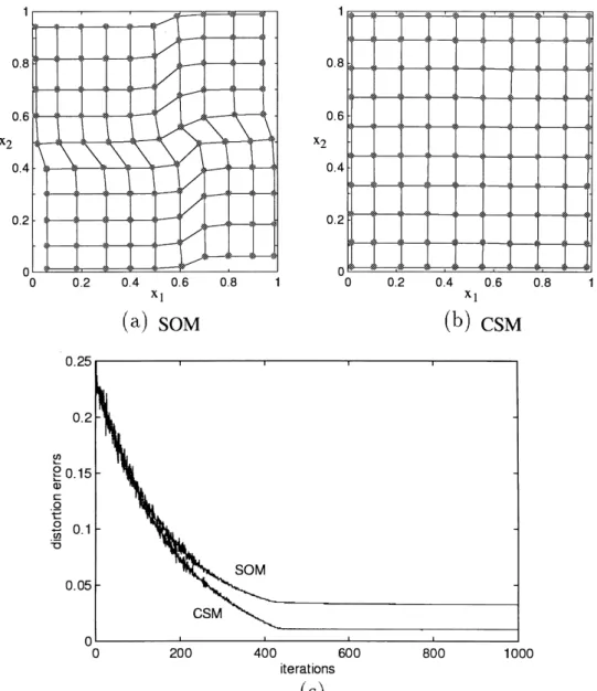
We tested the input set with 11× 11 input samples evenly distributed on the grid points of a unit square. Each model contained 10× 10 neurons. In Fig. 8(a) and (b), the maps trained by these two models have different ordering results. The SOM has crumples in the maps. The distortion errors are shown in Fig. 8(c).
We tested the inputs which were sampled from a square with uniform distribution. Fig. 9(a) shows the converged representation of the input data obtained using a 2D SOM
network with 10 × 10 neurons. Fig. 9(b) shows the results obtained by CSM. The distortion errors which occurred during the training iterations are plotted in Fig. 9(c).
When we used a linear neuron array with 30 neurons aligned in 1D, the results were as shown in Fig. 10. Fig. 10(a) and (b) shows the Voronoi tessellation of the input spaces partitioned by neurons. Fig. 10(b) shows a fine repre-sentation of the input space.
Fig. 11 shows a case where the inputs were sampled from a 3D half sphere. A network with 10 × 10 neurons was employed to approximate the surface of the 3D half sphere. Fig. 11(a) and (b) shows the trained results produced by the two models. As discussed by Li et al. (1993), the topology distortion shown in Fig. 11(a) and (b) comes from the discrepancy between the topology of the network and that of the surface. The distortion errors produced by the two models are plotted in Fig. 11(c).
Fig. 8. The trained network with 10× 10 neurons where 11 × 11 regular samples are used as inputs. (a) Using SOM; (b) using CSM; (c) the distortion errors which occurred during the adaptation.
To compare the computational costs between SOM and CSM, we record the execution time required for each simu-lation. The results are listed in Table 2. In each iteration, the computation cost of CSM is much more than that of SOM. This is because CSM computes the best-matching projected simplex s among all neighboring simplices of the winning neuron and solves the parameters in the mapping function Cs,s0.
The distortion errors produced by the two models indicate the performance of the synaptic weights in approximating the inputs. The results in all our simulations show that the distortion errors converged to different values in the two models. Before the convergence, the distortion errors in the CSM were similar to those in the SOM. From this obser-vation, we conclude that we can employ a hybrid model to reduce the amount of computation. The SOM can be
employed until there are no noticeable changes in the distor-tion errors. After this stage, the CSM can be employed.
From these results, we can see that the distortion errors produced by the CSM are usually smaller than those by the SOM at all iterations.
Let us examine the distortion errors in the continuous two-dimensional representation. For a sampled input x[ X, the SOM decides the synaptic weight vector wI(x) as the representation of x by Eq. (1). The distortion error, d1, can
be defined as the squared Euclidean distance in Rp:
d1 ix 2 wI xi 2
: 18
In the CSM, this input x is mapped to a best-matching projection vector y on one neighboring simplex s associated with the winning neuronI(x). The distortion error, d2, can Fig. 9. Trained network with 10× 10 neurons where inputs are sampled from a square with uniform distribution. (a) Using SOM; (b) using CSM; (c) the distortion errors which occurred during the adaptation.
be defined as
d2 ix 2 yi
2: 19
Consider four different cases for the projection y shown in Fig. 4. First, point x is in the simplex s. The value of the distortion error d2is equal to zero. The value of d1is greater
than zero except when x is equal to wI(x). In the second and third cases, where the projection is inside the simplex or on the boundary of the simplex, the vector x2 y is orthogonal to the vector y2 wi. The relationship
ix 2 wii
2 i x 2 y 1 y 2 w
ii 2 ix 2 yi21 iy 2 w ii 2 $ ix 2 yi2 20 is satisfied, i.e. d2# d1. In the last case, the distortion error
d2 is equal to the value of d1. The distortion error d2will
never be greater than the error d1. Note that deriving an
exact expression for the nonconformality measure (Reshetnyak, 1966) has been proven an illusive task. There-fore, we did not include it in. Instead, we use popular measure d1to show the learning behaviors.
5.2. Applications of the CSM
We will describe applications of the CSM to well-known tasks in biological image processing proposed by Thompson (1917), where the conformality requirement in biological morphology is addressed, and to tasks in geometrical surface mapping.
To solve the problem of biological form transformation from one species to another related species, conformality is required for similarity preservation in corresponding divi-sions. Harmonic correspondence (Thompson, 1917) of Fig. 10. Trained network with 30 neurons aligned in 1D where the inputs are sampled from a square with uniform distribution. (a) Using SOM; (b) using CSM; (c) the distortion errors which occurred during the adaptation.
related forms is a necessary part of the transformation. This correspondence can be found by means of the conformal mapping between the input space and the network field. Single transformation for the whole form was used in Thompson’s work for those species with simple relation-ships. The CSM can be used to map complex species harmonically.
This requirement necessitates the use of the CSM to model the mechanism of biological form transformation and distinguishes it from other continuous versions of the SOM. With this mechanism, the development of organisms, the evolution of biological forms, and form differences
between various species can be modeled. All these applica-tions have been developed in our laboratory in creating artificial creatures and in many other fields, such as cosme-tology, film conforming, and facial mapping. We will omit such detailed applications. Instead, we provide the follow-ing examples where one can have an insight into the proposed method.
In the study of biological morphology, Thompson (1917) first proposed that close topological similarity between quite different species can be related by coordinate transforma-tion. In his work, rectangular grids are placed on the whole form of one species. By means of coordinate transformation, both the grid and the form of this species are deformed to match the form of a related species. For continuity in the transformation, the conformal representation has been descriptively proposed to explore topological similarities between different species, such as the forms of fishes, the skulls of primates, and the carapaces of crabs. To carry out coordinate transformation, several techniques (Bookstein, 1978; Siegel & Benson, 1982) have been devised. These Fig. 11. Trained network with 10× 10 neurons where the inputs are sampled from the surface of a 3D half sphere. (a) Using SOM; (b) using CSM; (c) the distortion errors which occurred during the adaptation.
Table 2
Computational costs of each case in the simulations
Case SOM CSM
2D input, 2D network (Figs. 8 and 9) 10.1 min 121 min 2D input, 1D network (Fig. 10) 3.5 min 47 min 3D input, 2D network (Fig. 11) 13.2 min 195 min
techniques use specified landmarks over different forms, and the transformation retains mapped relationships between the corresponding landmarks.
There are problems involved in handling coordinates in complex cases (Huxley, 1932). One of the major problems is how to specify the topological similarity of the organisms appropriately and analytical wieldy (Medawar, 1945). Considering the interactions of neighboring cells in an organism (Turing, 1952) and the conformality in the form transformation, we devised this CSM to explore the topolo-gical relationships in the vicinal divisions (locally) in a form. Without marked points, the space-dependent confor-mal mapping functions from the input to the network field can be learned. Based on the learned results in the network fields for different forms, topological similarities and differ-ences between these forms can be compared.
To demonstrate the performance of the proposed model, we used it to simulate form transformations among various species of fishes. The images of adult fishes were sampled as the input data for seven species, respectively. The geome-trical forms of these fishes were quite different and complex. One form of a species was selected as the origin and trans-formed into those of the other six species. Fig. 12 shows the form of the selected fish.
For each species of fishes, the sampled image data were composed of 3-dimensional vectors, each of which contained the location coordinate and the intensity of a pixel in the image. We used a two-dimensional CSM (p 3 and q 2) with a general fish topology as shown in Fig. 13. There were 265 neurons regularly arranged in this network, which served as cartesian coordinates.
In the self-organization process of mapping each form of the seven species to this general network field, we settmax
1000,a(t) 0.05, h(d) exp( 2 d2/2gN2), N 20, and
g t 0:001t=tmax g(t) 0.001t/tmax. The initial network
network fields.
Fig. 14(a)–(f) shows the mapped results for the form transformations of the selected fish to the other six fishes. The transformed form which was mapped from that of the selected fish via the network field is shown in the figure. From these results, we observe the topological similarities and differences between the forms of the various species. All these form transformations are quite harmonic.
In addition to the biological morphology, there are many other potential fields to apply this model. We studied the shape transformations between different geometrical surfaces. Fig. 15 shows the mappings among three different shapes, a circle, a triangle with curved edges, and a penta-gram. Using the CSM, we constructed conformal transfor-mations among them. A two-dimensional square network with regularly arranged 20× 20 neurons was used in these simulations. The training parameters were set to the same values as those used in the above simulations.
Similarly, we can apply CSM to simulate the biological growth and development. In artificial life applications, the sudden surface warps during an artificial object motion or growth can be modeled and followed by the proposed mapping. With such mapping one can map all local surface properties, such as colors, to their corresponding areas. All local growth properties can be identified and monitored
Fig. 13. The topology of the network with 265 neurons for the form transformation.
Fig. 14. The image of the form transformed from that of the selected fish via the CSM. (a) Oncorhynchus masou formosanum; (b) Epinephelus
brun-neus and; (c) Acanthopagrus schlegeli; (d) Pempheris oualensis; (e) Chae-todon auripes and; (f) Cypselurus katoptron.
during growth. We now give an example. We sample two facial images of one person at different ages. We employ a two-dimensional CSM network with a circular topology. There are 344 neurons regularly arranged in this network. Using the CSM results of mapping these two images, we can sample the intermediate images at different stages. Fig. 16(a)–(f) shows the results of the simulated growth and development. The four images, 16(a), 16(c), 16(d), and 16(f), are sampled during the evolution of the mapping process when we map the 16(b) image toward the 16(e) image using CSM. To our knowledge, this kind interpola-tion and extrapolainterpola-tion of whole images has not been studied before.
One goal of the project is to develop an autonomous facial mapping technique which can be used to map two given or user defined 3D face meshes such that a facial expression in one mesh can be transferred to another mesh automatically. This kind development can facilitate many facial systems to exchange facial data. The examples in Figs. 14 and 15 can justify this development. Next, we show a much more difficult task. A 2D facial image sampled from video records can be mapped to a given 3D face mesh. We use a two-dimensional CSM network with a circular topology. There are 344 neurons regularly arranged in this network. The input vectors of the image and the mesh contain different information, the intensity value at 2D plane and 3D spatial coordinates, respectively. Fig. 17 shows the mapping results. The mapping from a 2D facial picture to a 3D head surface is shown in the figure. With such technique, one can map arbitrary 2D facial image to any 3D face mesh. This mesh then carries and follows the user facial image in a Karaok performance. This kind appli-cation is different from those finding 3D images based on two video records at different angles.
6. Conclusions
The conformal transformation has been used in different fields, for example, biological modeling, fluid dynamics, and cartography. The intention to construct this specific transformation inspires us to devise the CSM. As shown in our simulations, the CSM network provides conformal transformation for biological morphology and geometrical
mapping. The proposed network meets the conformality requirement closely.
We equip the network with the simplicial representation to partition the continuous space of the network field. Then the analytic one-to-one correspondence by spanning the field in the input space is developed. The conformality prop-erty which characterizes the SOM is further preserved in the Fig. 15. The learned mappings between a circle (a) and a triangle with curved edges (b), and a pentagram (c).
Fig. 16. The simulated biological growth and development, (a) the simu-lated image at 8 years old; (b) the real image at 13 years old; (c) the simulated image at 18 years old; (d) the simulated image at 23 years old; (e) the real image at 28 years old, and; (f) the simulated image at 33 years old.
detailed representation. So far, this continuous conformal mapping from the input space to the network field has not been explored by existing SOMs. This conformality requirement necessitates the use of the proposed network and distinguishes it from the SOMs.
In simulations, we apply the CSM to solve the morpholo-gical shapes between forms. Different from all other methods, the CSM needs no marked points to establish the space-dependent conformal functions to map the topological similarities between two forms. Various form trans-formations can be realized by the CSM. These results verify the performance of the proposed model.
The computation cost of CSM includes the searching of all neighboring simplices and the solving of ODEs for each simplex. This cost is heavy in many real time applications. Reducing the network density will linearly reduce the cost. The conformality constraint is still satisfied for a reduced sparse network. A sparse network with such constraint may deviate the mapping. The proposed technique may not serve as a powerful technique to reduce the network density. The focus is on autonomous mapping, interpolating, and extra-polating those surface which have conformal properties such as surfaces in morphology. This autonomous bio-shape mapping has received intensive studies in modern artificial life applications.
References
Bookstein, F. L. (1978). The measurement of biological shape and shape
change, Lecture notes in biomathematics, 24. Berlin: Springer.
Davis, P. J., & Rabinowitz, P. (1984). Methods of numerical integration, Orlando: Academic Press.
Henrici, P. (1974). Applied and computational complex analysis, New York: Wiley.
Huxley, J. S. (1932). Problems in relative growth, London: Methue. Kohonen, T. (1982). Self-organized formation of topologically correct
feature maps. Biological Cybernetics, 43, 59–69.
Kohonen, T. (1993). Physiological interpretation of the self-organizing map algorithm. Neural Networks, 6, 895–905.
Lemmon, M. (1994). Topologically ordered competitive sampling. Neural
Network, 7, 101–111.
Li, X., Gasteiger, J., & Zupan, J. (1993). On the topology distortion in self-organizing feature map. Biological Cybernetics, 70, 189–198. Medawar (1945). Essays on growth and form, Oxford.
Munkres, J. R. (1984). Elements of algebraic topology, MA, USA: Addison-Wesley.
Reshetnyak, Y. G. (1966). Estimates of the continuity modulus for various mappings (Eq. (2). Sibirskii Matematicheskii Zhurnal, 7, 1106–1114. Ritter, H. (1993). Parameterized self-organizing maps. In:
ICANN93-Proceedings (pp. 568–575), Amsterdam.
Siegel, A. F., & Benson, R. H. (1982). A robust comparison of biological shapes. Biometrics, 38, 341–350.
Tanaka, T. (1994). On evaluation of reference vector density for self-organizing feature map. IEICE Transactions, Information and Systems,
E77-D, 402–408.
Thompson, D. A. W. (1917). On growth and form, Cambridge: Cambridge University Press.
Trefethen, L. N. (1980). Numerical computation of the Schwarz– Christoffel transformation. SIAM Journal on Scientific and Statistical
Computing, 1, 82–102.
Turing, A. M. (1952). The chemical basis of morphogenesis. Philosophical
Transactions of the Royal Society, 237, 37–72.
Fig. 17. The geometrical mapping from a 2D facial picture (a) to a 3D surface (b). (c) The mapped 3D picture.