THE ANALYSIS OF STRAIN DATA OF THE MONITORING SYSTEM
IN THE CHIANG-KAI-SHEK INTERNATIONAL AIRPORT
Chia-pei CHOU Professor
Department of Civil Engineering National Taiwan University
No.1, Sec.4, Roosevelt Rd., Taipei 106, Taiwan, R.O.C.
Fax: +886-2-23639990 E-mail: [email protected]
Shih-ying WANG Ph. D. Student
Department of Civil Engineering National Taiwan University
No.1, Sec.4, Roosevelt Rd., Taipei 106, Taiwan, R.O.C.
Fax: +886-2-23639990
E-mail: [email protected]
Abstract: In January 2002, a research experiment installed a number of sensors in taxiway
N1 in the northern field of the Chiang-Kai-Shek (CKS) International Airport during a scheduled slab repair. The sensors measure changes of slab behavior in response to various environmental factors and different aircraft loading. The slabs are 6 m wide, 7 m long and with 41 cm in depth. A total of 102 monitoring devices were installed. These included the H-bar and the Dowel-bar strain gauges; position gauges, temperature gauges, and moisture gauges; as well as optical fiber sensors. This paper mainly focuses on the analysis of the instant data recorded by H-bar strain gauges generated by the taxing aircraft, including the variation of strain induced by aircraft of different gear configurations, the strain at different depths and the joint, as well as the comparison between the finite element method (FEM) analysis results and the field data.
Key Words: monitoring system, strain, FEM
1. H-BAR STRAIN GAUGE POSITIONING AND DATA PROCESSING
Gauge positions of this CKS International airport project are displayed in Figure 1. A total of 42 H-bar strain gauges are installed in slabs #3, #6, and #7. Each H-bar strain gauge is assigned a unique code. The first digit refers to the slab number. The letter H stands for the H-bar strain gauge, the first digit after letter H identifies the sequence no. of strain gauges, and the next digit indicates the depth of the gauge (i.e. 1 is at slab top, 2 is in the mid-depth, and 3 is at slab bottom). If the code ended with letter V, indicates that the strain gauges aligned with the taxing direction (the y axis). Otherwise, the H-bar strain gauges are positioned perpendicular to the taxing direction (the x axis). For example, 6H71 indicates an H-bar strain gauge installed in slab 6, group 7, at slab top(5cm from the surface), and perpendicular to the taxing direction. In this study, 6H7 has 3 separate gauges, top, mid-depth, and bottom, for both x and y directions while the others are installed at top and bottom locations only.
5
6
7
5S1 6S1 6H2 5S2 6S2 6T2 6M23 6H4 6T21~6T27 6H41 6H43 6H41V 6H43V 6H21 6H23 6H3 6H31 6H33 6T1 6T11~6T17 6M1 6M11 6M13 6H5 6H51 6H53 6H51V 6H53V 6H6 6H61 6H63 6H61V 6H63V 6S3 7S3 6H7 7H9 7H91 7H93 7H91V 7H93V 6S4 7S4 6H8 7H10 7H11 6H81 6H83 6H81V 6H83V 7H101 7H103 7H101V 7H103V 7H111 7H113 7H111V 7H113V 6H71 6H72 6H73 6H71V 6H72V 6H73VData acquisition system 1. Dowel-bar Strain gage
2. H-bar strain gage 3. Temperature sensors 4. Moisture sensors 5. Position gages 6. Optical Fiber sensors
Sensor Quantity
Label
H-bar strain gage 2
6H2
H-bar strain gage 4
3H1
H-bar strain gage 2
6H3
H-bar strain gage 4
6H5
H-bar strain gage 4
6H4
H-bar strain gage 4
6H6
H-bar strain gage 4
6H8
H-bar strain gage 6
6H7
H-bar strain gage 4
7H9
H-bar strain gage 4
7H11
H-bar strain gage 4
7H10
Dowel-bar Strain gage 4 S1 Dowel-bar Strain gage
4 S2
Dowel-bar Strain gage 4 S4
Dowel-bar Strain gage 4 S3 Temperature sensors 7 6T1 Temperature sensors 7 6T2 Moisture sensors 2 6M1 Moisture sensors 1 6M2 Position gages 20 3H1 3H11 3H13 3H11V 3H13V
1
2
3
95 cm 98cm 88.5cm 31.5cm 30.5cm 98cm 98cm 90cm 90cm 72.5cm 3.2m 1 5 6 3 7 2 8 4 Runway 05-23 NC Taxiway N1 Taxiwayx
y
CenterlineThe locations of H-bar strain gauges were determined based on the main gear configuration of B747-400. Therefore, when a B747-400 aircraft taxis along the centerline of the N1 taxiway, the main gears will pass over 7H9, 7H11, 6H7, 7H10, 6H8, 6H2, and 6H3 in sequence. Besides, this research also installed two groups of H-bar strain gauges (6H4 and 6H6) on the edge and one group (6H5) in the center to observe the strain variations in different locations of the slab.
H-bar strain gauges are designed to measure static strain at 0.1 Hz as well as dynamic strain at 100 Hz respectively. The static data are recorded over a long period of time, but the dynamic data are stored only when aircraft taxis by. The impact of aircraft must be filtered when the static data is processed. Likewise, in order to eliminate the influence of the environmental effect the beginning of each dynamic data file before aircraft arrival must be set to 0 for analyzing the dynamic effects from the aircraft. This paper will focus on the analysis of the dynamic data namely the behavior of slabs when aircraft pass.
2. LITERATURE REVIEW
Due to the theoretical analysis and material property tests in the laboratory over a long period of time, many rigid pavement monitoring projects are proceeded recently to observe the behavior of slabs resulted form aircraft loading and environmental effects. The Airport Technology Research and Development Branch of Federal Aviation Administration (FAA) undertook several airport pavement researches. Among them, the Airport pavement Instrumentation Project at the Denver International Airport and the tests in the National Airport Pavement test Facility (NAPTF) focuses on the rigid pavement. Kapiri, M. et al. compared the field data of the Denver International Airport and the simulation result of ICM (Integrated Climatic Model) V.2. By doing this, the load transfer efficiency (LTE) in different climates was discovered. Hayhoe, G. F. et al. used the data measured in the NAPTF to analyze the interaction between the gear, wheel base, and pavement, to find out the differences between the pavement behavior when taking static loading and dynamic loading. Guo, E. H.
et al. in the NAPTF conducted experiments on three different pavement types and added loads
with gears of four or six wheels (each weighs 45,000 lbs.). Because some corner cracks happened in the initial stage of the experiment, the researches learned the strain appearance when corner cracks happened from the recorded strain data.
Kukreti, A.R. et al. applied finite element method (FEM) to the dynamic analysis of discontinuous rigid pavement in the airport. The results show that the deflection caused by static loading is larger than that of dynamic loading. When the slab takes dynamic loading, the deflection will increase due to the increase of the moving speed of aircraft. Masad, E. et al.
discussed the behavior of jointed rigid pavement affected by the temperature variation. A three-dimension model of four slabs was built by using ABAQUS software. This model aimed at observing the superposition of curling stress and horizontal temperature stress as well as the opening of joints. The results show that the value of adding up curling stress and horizontal temperature stress is smaller than the superposition value calculated by the software. The tensile stress calculated within the nonlinear temperature gradient is larger than that within the linear one, and the difference is 3 to 13% of tensile strength.
To sum up, researchers analyze the behavior of rigid pavement more by simulation software. Only FAA has rich experiences on large scale field tests in airport, and keeps for a long time. It indeed exist some differences between field measurements and simulation results. Therefore, it is encouraged that more researches are needed to figure out the field behavior of rigid pavement.
3. THE STRAIN TYPES OF DIFFERENT MAIN GEAR CONFIGURATIONS
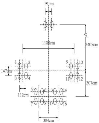
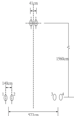
Due to different aircraft types and manufacturers, the main gear configurations are diverse. Although the H-bar strain gauges were embedded based on the gear configuration of B47, the following analysis will focus on the real time strains caused by the loading of B777-300 and B737-800 in additional to B747 taxing over the N1 taxiway in the CKS International Airport. The path of each aircraft is orientated based on the results of aircraft positioning tests. These tests used the theodolite to track the path of nose gears, and then calculated the location of main gears according to the path and the main gear configuration. The main gear configurations of three different aircraft are shown in Figure 2, 3, and 4.
Figure 5 shows the strain variation measured by 6H81 when slab 6 was loaded by a B747-400 aircraft. Gauge 6H81 is located directly under the path of tandem gear of wheels 5-6 and 7-8 (as shown in Figure 2) of a B747-400 aircraft when it taxis along the centerline of the N1 taxiway. The first peak tensile strain in Figure 5 was measured when the nose gear rolled on slab 2. Due to the load transferred through the joint and a relatively large distance between the nose gear and the gauge, 6H81 recorded a tensile strain. The second tensile strain was recorded when tandem gear of wheels 1- 2 and 3- 4 passed the same transverse section of 6H81. While tandem gear of wheels 5-6 and 7-8 passed over 6H81, the strain gauge recorded two peak compressive strains which are -7.76*10-6 and -8.79*10-6.
384cm 112cm 147cm 307cm 1100cm 2407cm 91cm 1 16 15 14 13 12 11 10 9 8 7 6 5 4 3 2
Figure 2. The Gear Configuration of B747-400
1097cm 3122cm 78cm 140c m 290cm 145cm 1 2 12 10 8 11 9 7 6 5 4 3
572cm
1560cm 41cm
140cm
1 2 3 4
Figure 4. The Gear Configuration of B737-800
-10 -8 -6 -4 -2 0 2 4 6 8 10 04 .98 06 .44 07 .90 09 .36 10 .82 12 .28 13 .74 15 .20 16 .66 18 .12 19 .58 21 .04 22 .50 23 .96 25 .42 26 .88 28 .34 29 .80 31 .26 32 .72 34 .18 35 .64 37 .10 38 .56 40 .02 41 .48 42 .94 44 .40 45 .86 Time(sec) Stra in (1 0 -6) 6H81
Figure 5. The Strain Variation Recorded by 6H81 When B747-400 Passes over
Figure 6 illustrates the strain variation recorded by 6H71 when slab 6 was loaded by a B777-300 aircraft. The three peak compressive strains in Figure 6 were measured when the main gears of B777-300 passed slab 6. They are -4.57*10-6, -5.15*10-6, and -4.85*10-6.
-6 -4 -2 0 2 4 6 01 .1 2 01 .2 3 01 .3 4 01 .4 5 01 .5 6 01 .6 7 01 .7 8 01 .8 9 02 .0 0 02 .1 1 02 .2 2 02 .3 3 02 .4 4 02 .5 5 02 .6 6 02 .7 7 02 .8 8 02 .9 9 03 .1 0 03 .2 1 03 .3 2 03 .4 3 03 .5 4 03 .6 5 03 .7 6 03 .8 7 03 .9 8 04 .0 9 Time(sec) S tra in (10 -6) 6H71
Figure 6. The Strain Variation Recorded by 6H71 When B777-300 Passes over
Figure 7 displays the strain variation recorded by 6H81 when slab 6 was loaded by a B737-800 aircraft. The peak compressive strains -1.44*10-6 in Figure 7 were measured when the main gears of B737-800 passed slab 6.
-4 -3 -2 -1 0 1 2 3 4 24 .14 24 .74 25 .34 25 .94 26 .54 27 .14 27 .74 28 .34 28 .94 29 .54 30 .14 30 .74 31 .34 31 .94 32 .54 33 .14 33 .74 34 .34 34 .94 35 .54 36 .14 36 .74 37 .34 37 .94 38 .54 39 .14 39 .74 40 .34 40 .94 Time(sec) Stra in (1 0 -6) 6H81
By observing Figures 5 to 7, the main gear configuration could be easily identified, so as the aircraft types. To assume that main gears carry 95% of total weight of an aircraft, the single axle loads of the B747-400, B777-300, and B737-800 aircrafts discussed in this paper are calculated as 42 tons, 38 tons, and 32 tons respectively with known gross weight of each aircraft. However, the ratios of maximum compressive strains shown in Figures 5 to 7 do not give the same readings as 42/38, 42/32, or 38/32. It is mainly because that the main gears of aircraft B777-300 and B737-800 do not follow the same path of B747-400, therefore, those main gears do not pass over the gauge 6H8 directly. This results in relatively small measurements of compressive strains. Nevertheless, the tendency of heavy axle load inducing high stress in concrete slab can obviously be found in those figures.
4. THE STRAIN TYPES OF DIFFERENT DEPTHS AND LOCATIONS IN THE SLAB
This section will emphasize on the strain variation in the same point but at different depths as well the differences of strains at both sides of a joint when aircraft crosses the joint.
4.1 The Strain Variation at Different Depths
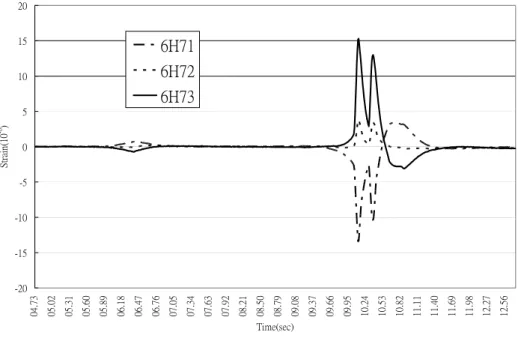
As mentioned in the first part of this paper, the experiment installed 3 gauges from top to bottom at 6H7 location along the slab depth for both x and y directions. A typical measuring output during a B747-400 aircraft passed over is chosen to interpret the strain measured by 6H7. As Figure 8 displays, 6H71 and 6H73 measured tensile and compressive strain respectively when the nose gear passed slab 2. While tandem gear of wheels 1-2 and 3-4 of B747-400 aircraft passed over 6H7, 6H71 recorded two peak compressive strains, -13.41*10-6 and -10.43*10-6, and 6H73 recorded two peak tensile strains, 15.30*10-6 and 12.70*10-6. Thus it can be seen that the strains in the top and bottom of a slab are symmetric. The strain gauge in the mid-depth, 6H72, was designed in the neutral axis of the slab with expected zero or very small measured strain. However, the readings in Figure 8 show that there are two peak tensile strains, 3.60*10-6 and 3.38*10-6, recorded by 6H72 which indicate that the neutral axis is above the mid-depth of concrete slab.
-20 -15 -10 -5 0 5 10 15 20 04 .7 3 05 .0 2 05 .3 1 05 .6 0 05 .8 9 06 .1 8 06 .4 7 06 .7 6 07 .0 5 07 .3 4 07 .6 3 07 .9 2 08 .2 1 08 .5 0 08 .7 9 09 .0 8 09 .3 7 09 .6 6 09 .9 5 10 .2 4 10 .5 3 10 .8 2 11 .1 1 11 .4 0 11 .6 9 11 .9 8 12 .2 7 12 .5 6 Time(sec) St ra in (10 -6 ) 6H71 6H72 6H73
Figure 8. The Strain Variation Recorded by 6H7 When B747-400 Passes over
4.2 The Strains at the Joint
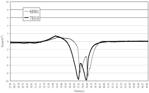
This research designed two paired strain gauges located at both sides of joint of slabs 6 and 7, 6H7 and 7H9 as well as 6H8 and 7H10. This special design was designated to study the strain variation while an aircraft across the joint. By comparing the strains obtained from both sides of the joint the load transfer effect in horizontal strain rather than in vertical deflection can be evaluated. Again, typical aircraft B747-400 as selected in previous study is used to illustrate this analysis. Figure 9 represents the strains measured by 7H91 and 6H71 while Figure 10 displays the strains recorded by 7H101 and 6H81 when a B747-400 is rolling over from slab 7 to slab 6. While axle of wheels 1-2 first passes over 7H9, the first peak reading of compressive strain is recoded as -8.13*10-6 at 7H91, the gauge placed at the top. The second compressive strain is recoded about 1.5 second afterward with a similar reading, when axle of wheels 3-4 moves on 7H9. From the recorded data the approximately aircraft rolling speed can be computed as 3.44 km per hour. Likewise, tandem gear of wheels 5-6 and 7-8 passes over strain gauges 7H10 and 6H8. A similar diagram is shown in Figure 10. However, the maximum compressive strains recorded in Figure 10 are higher those in Figure 9. It is very clear to observe that the tandem gear load of wheel 5-6 and 7-8 is heavier than that of tandem gear of wheels of 1-2 and 3-4. This is different from the assumption used for most of the airport design that all the wheels share equally the 95% of the gross aircraft weight. It also should be noted that there exists a tensile strain for both 6H71 and 7H91 after the two peak readings of compressive strain (Figure 9). Contrarily, a tensile strain appears ahead of the two peak readings of compressive strain for both 6H81 as well as 7H101 (Figure 10).
Tensile strains of 6H81 and 7H101 are induced by the tandem gear of wheels 1-2 and 3-4 when those wheels are crossing the joint of slabs 7 and 6. Due to the distance of 358 cm between the center to center of these dual tandem gears, a reverse strain/ stress is induced at the slab top when wheel loads applied on the pavement. Similarly, the tensile strains observed at 6H71 and 7H91 are induced by the tandem gear of wheels 5-6 and 7-8 when those wheels are moving over the same joint.
-10 -8 -6 -4 -2 0 2 4 6 8 10 23.98 24.76 25.54 26.32 27.10 27.88 28.66 29.44 30.22 31.00 31.78 32.56 33.34 34.12 34.90 35.68 36.46 37.24 38.02 38.80 39.58 40.36 41.14 41.92 42.70 43.48 44.26 45.04 45.82 Time(sec) Stra in(10 -6) 6H71 7H91
Figure 9. The Strain Variation Recorded by 6H71 and 7H91
-10 -8 -6 -4 -2 0 2 4 6 8 10 27. 98 28. 57 29. 16 29. 75 30. 34 30. 93 31. 52 32. 11 32. 70 33. 29 33. 88 34. 47 35. 06 35. 65 36. 24 36. 83 37. 42 38. 01 38. 60 39. 19 39. 78 40. 37 40. 96 41. 55 42. 14 42. 73 43. 32 43. 91 44. 50 45. 09 45. 68 46. 27 46. 86 Time(sec) Stra in(10 -6) 6H81 7H10
The taxiing direction of this B747-400 aircraft was from slab 7 to slab 6, thus the first peak compressive strain always firstly appears at 7H91 as well as 7H101. At the mean time readings recorded from 6H71 and 6H81 are relatively smaller than those from 7H91 and 7H101 due to the load transferring from the joint. By comparing the readings at both sides load transfer effect can be evaluated in another form as the ratio of compressive strain before and after joint. This definition provides more meaningful information for joint load transfer than the traditional comparison of deflection. In this field, it is found that the load transfer effects calculated in this way are 48.57% and 56.09% for the joint of slabs 7 and 6.
5. THE COMPARISON BETWEEN THE FIELD TEST DATA AND FEM SIMULATION RESULTS
This section will analyze some field test data first, and then introduce the finite element method (FEM) model developed by this research study. Finally, the comparison between the field test data and FEM simulation results is demonstrated.
5.1 The Analysis of Field Test Data
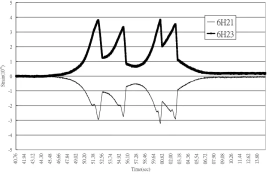
This research conducted a precision location test by using the fire engine and tanker trucks of the CKS International Airport. This test aimed at evaluating the relationship between the loading location and the strain measured as well as the dynamic and static loading data; moreover, comparing the field test data and FEM simulation results. Figure 11 illustrates the strain variation of 6H2 when the tanker with two tandem axles moved over directly on the top of it. Because 6H2 was installed right in front of joint of slab 5 and slab 6 and the truck would pass over 6H2 before the joint, it can be noted that there is a steep decrease point after each peak strain. This clearly reveals the influence caused by the discontinuity of joint.
Figure 12 shows the relation between the position of the truck and the strain recorded by 6H2 at any given time point, and the positions were decided based on the moving speed of the truck. The zero point on the transverse axle means the joint between slab 5 and slab 6, and the number on the X-axis indicates the distance between the first axle of the truck and the joint. The reading of the first peak tensile strain on the transverse axle is -30.17 cm, and it is the same distance between 6H2 and the joint. Further, the starting point that the loading begins to influence the reading of 6H2 is about 380 cm away from the joint, i.e. 350 cm away from 6H2.
-5 -4 -3 -2 -1 0 1 2 3 4 5 40.76 41.9 4 43.12 44.30 45.4 8 46.66 47.8 4 49.02 50.20 51.3 8 52.56 53.74 54.9 2 56.10 57. 28 58.46 59.64 00.8 2 02.00 03.18 04.3 6 05.54 06.7 2 07.90 09.08 10.2 6 11.44 12.62 13.8 0 Time(sec) S tra in (1 0 -6) 6H21 6H23
Figure 11. The Strain Variation Recorded by 6H2 during the Movement of Tanker
-4 -3 -2 -1 0 1 2 3 4 -48 0 -46 0 -44 0 -42 0 -40 0 -38 0 -36 0 -34 0 -32 0 -30 0 -28 0 -26 0 -24 0 -22 0 -20 0 -18 0 -16 0 -14 0 -12 0 -10 0 -8 0 -6 0 -4 0 -2 0 0 20 40 60 80 10 0 12 0 14 0 16 0 18 0 20 0 22 0 24 0 26 0
Distance to the joint(cm)
S tra in (10 -6) 6H21 6H23
Figure 12. The Strain Variation Recorded by 6H2 – Based on the Distance to the Joint
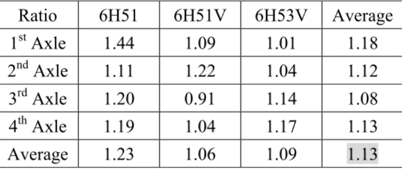
In the field test, tanker with full tank of water was arranged to move slowly on the experimental slabs first. Dynamic strains were recorded under the movement of truck. Then the truck was moved on the surface of the exact position of 6H51 and stayed still. The static strains were recorded under this condition. Table 1 shows the ratios of the static to dynamic strain caused by the tanker. Most ratios in the table are greater than 1, and the
Joint 6H2
Salb 5 Salb 6
average ratio is 1.13. Thus, it can be concluded that the strain caused by static loading which is simulated by FEM would be greater than that caused by dynamic loading, with 10 to 15 % in this case.
Table 1. The Ratios of Static Strain to Dynamic Strain
Ratio 6H51 6H51V 6H53V Average 1stAxle 1.44 1.09 1.01 1.18 2ndAxle 1.11 1.22 1.04 1.12 3rdAxle 1.20 0.91 1.14 1.08 4thAxle 1.19 1.04 1.17 1.13 Average 1.23 1.06 1.09 1.13
5.2 The Comparison of Field Test Data to the FEM Simulation Results
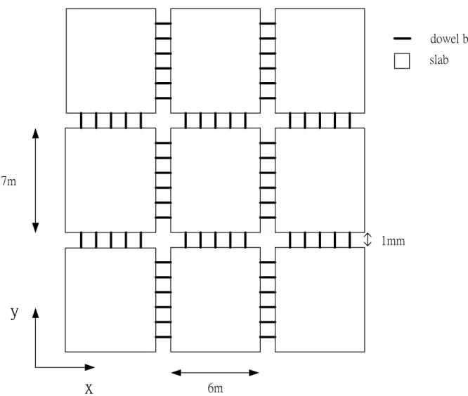
The model constructed by this study contained the slab, subbase, subgrade, and dowel bar. The shell element was adopted to describe the behavior of slab, the spring element was introduced to simulate the modulus of subgrade reaction of subbase and subgrade, and the beam element was characterized as dowel bar. Hence, this FEM is developed as a two-dimensional model.
There are a total number of 9 slabs constructed in this model, and the dimension of one slab was 6m*7m. The joints were assumed as 1mm in width, and slabs were 41 cm in depth. The element type of slabs was S4R5, the Young’s modulus was 6*106 psi (the laboratory test value), and the poisson ratio was 0.15. The element type of dowel bars was B31. The diameter, 3.2 cm, was the same as that used in the actual slabs, the Young’s modulus was 2.9*107 psi, and the poisson ratio was 0.3. This research assumed that the slabs were on the Winkler foundation, and the modulus of subgrade reaction was acted at the node. SPRING1 was introduced to simulate the subgrade reaction, and the k value was 600 pci. The illustration of this FEM model is shown in Figure 13.
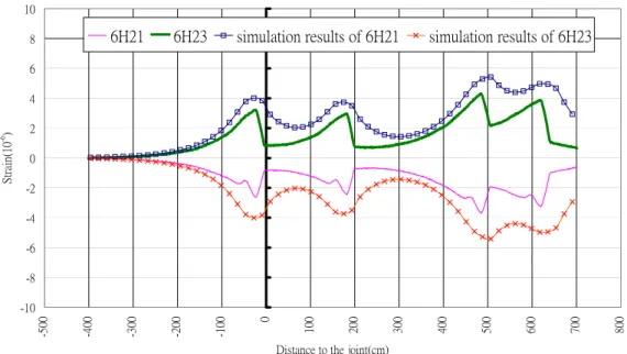
This FEM model was used to simulate the static loads of tanker continuously by moving the truck position with a small interval from slab 7 to 6. The four peak strains in Figure 14 stands for the strains caused by the four axles of the tanker, and the transverse axle means the distance of the first axle to the joint. The recorded strain data (dynamic) and the simulation results (static) are very much similar, and they both represent that the strains caused by the two rear axles are greater than those cause by the two front ones. To compare the peak values
of simulation and field strains of 6H21, it can be seen that ratio of simulation (static) to field strains (dynamic), 1.2, is close to the ratio of static to dynamic strains shown in Table 1. Hence, by using the tire pressure divided by the static to dynamic ratio, 1.2, the simulation results are displayed in Figure 15. The curves of the field data and the revised simulation results are even closer. Thus, it can be concluded that the dynamic loading can be simulated by the means of dividing the static loading by a ratio, say 1.2.
According to the above analysis, the measured data can be adopted to calibrate the parameters used in the FEM model, and the revised model is able to simulate the strain caused by the loading effectively.
x
y
1mm 7m 6m dowel bar slab-10 -8 -6 -4 -2 0 2 4 6 8 10 -500 -400 -300 -200 -100 0 100 200 300 400 500 600 700 800
Distance to the joint(cm)
Strain(10
-6 )
6H21 6H23 simulation results of 6H21 simulation results of 6H23
Figure 14. The Comparison between Field Test Data and Simulation Results-1
-10 -8 -6 -4 -2 0 2 4 6 8 10 -500 -400 -300 -200 -100 0 100 200 300 400 500 600 700 800
Distance to the joint(cm)
Strain(10
-6 )
6H21 6H23 simulation results of 6H21 simulation results of6H23
Figure 15. The Comparison between Field Test Data and Simulation Results-2
6. CONCLUSION
1. By observing the instant data measured by H-bar strain gauges, the main gear configurations can be easily identified.
2. When the installed location of H-bar strain gauges is loaded by the aircraft, the strain gauge at the bottom would measure tensile strain, and the magnitude would be related to the location and the intensity of the loading.
3. The strains of different depths in the same location correspond to the theoretical assumption, but the depth of the neutral axis is above the mid-depth of concrete slab. 4. The joint transfer effect is defined based on the strain data measured by the strain gauges
at both sides of the joint at the same moment when loads are applied at one side of the joint. This is an alternative way for describing the load transfer capability.
5. The time point when the peak strain happened could be used to figure out the location of the loading.
6. According to the field test results, the strain caused by static loading is larger than that caused by dynamic loading, and the ratio of static load to dynamic load is around 1.13. 7. The FEM model developed in this study is capable of estimating the strain of slabs caused
by loading effectively.
REFERENCES
Guo, E. H., Hayhoe, G. F. and Brill, D. R. (2002) Analysis of NAPTF traffic test data for first-year rigid pavement test items. the 2002 FAA Airport Technology Transfer
Conference.
Hayhoe, G. F., Cornwell, R. and Garg, N. (2002) Slow rolling responses tests on the test pavements at the National Airport Pavement Test Facility (NAPTF). NAPTF Website.
Kapiri, M., Tutumluer, E. and Barenberg, E. J. (2002) Analysis of temperature effects on pavement response at Denver International Airport. Proceedings-International Air
Transportation Conference.
Kukreti, A. R., Taheri, M. R. and Ledesma, R. H. (1992) Dynamic analysis of rigid airport pavements with discontinuities, Journal of Transportation Engineering, Vol. 118, No. 3, May-Jun.
Masad, E., Taha, R. and Muhunthan, B. (1996) Finite-element analysis of temperature effects on plain-jointed concrete pavements, Journal of Transportation Engineering.