基於有號距離的區間值模糊集合的排序

行政院國家科學委員會專題研究計畫 成果報告

基於有號距離的區間值模糊集合的排序

中 華 民 國 94 年 12 月 21 日

Ranking of Interval-Valued Fuzzy Sets Based on Signed Distance

by Kweimei Wu

Department of Mathematics, National Taiwan University Taipei, Taiwan

Ranking of Interval-Valued Fuzzy Sets Based on Signed Distance

by Kweimei Wu

Department of Mathematics, National Taiwan University Taipei, Taiwan

Abstract:

In this article, we use the signed distance to consider the ranking problem of interval-valued fuzzy sets. This ranking can be used in decision-making problem based on interval-valued fuzzy sets, or in the fuzzification or defuzzification of two sides of an equation in the fuzzy sense. We can learn that how far it is between two interval-valued fuzzy sets by the ranking of the signed distance.

§1. Introduction

In Yao and Wu [ 12 ], we considered the family FN of the fuzzy numbers in R which

are convex and normal, and also defined the signed distance and ranking of the fuzzy numbers on FN. In section 3 of [ 12 ], we compared the ranking using the

signed distance in [12] with the ranking of [ 2, 3, 4, 6, 7, 11 ]’s. All the ranking’s in papers [ 2, 3, 4, 5, 6, 7, 8, 10, 11, ] are dealing with the fuzzy numbers which are different from the ranking interval-valued fuzzy sets in this paper. It ought to use interval-valued fuzzy set to handle the practical situation in order to fit the reality. In the inventory problem for some material discussed in Yao and Su [ 13 ], to find out the exact value r0 of the total demand during the period of time T is rather

difficult, but it would be easier to know the total demand ” around r0 ” ( which is a

fuzzy language ). Since the membership grade of r0 during the time period T may

not equal to 1, therefore assume it belongs to the interal [λ, 1], 0 ≤ λ ≤ 1. Thus they could express it in the fuzzy language ” around r0 ” by using an interval-valued

fuzzy set. As we mentioned in Abstract, an interval-valued fuzzy sets is needed in the discussion of decision-making problem. These, bring us to discuss the problem of how to rank the interval-valued fuzzy sets.

In section 2, we use the method of signed distance similar to the one in [ 12 ] to define the ranking of interval-valued fuzzy sets. Then we have some results closed to the properties of signed distance ranking over R.

with [ 6, 7, 12 ]’s works as well as to the Yager’s [ 11 ].

§2. Ranking of Interval-valued Fuzzy Sets.

In this paper, we consider the problem for ranking of interval-valued fuzzy sets as follows:

Definition 1. An interval-valued fuzzy set (i-v fuzzy set for short ) A on R is given by

A = { x, [ µ∆ _AL(x), µ_AU(x) ]}, x ∈ R or A = [AL, AU] (1)

where 0 ≤ µ_AL(x) ≤ µ_AU(x) ≤ 1 ∀x ∈ R

Let µ_A(x) = [ µ_AL(x), µ_AU(x) ], x ∈ R , then the grade of membership of the i-v fuzzy set A at x belongs to the interval [ µ_AL(x), µ_AU(x) ].

Insert Fig. 1 here

Let us assume the i-v fuzzy set A satisfies the following conditions: (1◦_{) µ}

AL(x; λ), µAU(x; ρ) are continuous functions of x in R. ( see Fig.1 )

(2◦_{) max}

xµ_AL(x; λ) = λ, maxxµ_AU(x; ρ) = ρ, 0 < λ ≤ ρ ≤ 1 and 0 ≤ µ_AL(x; λ) ≤ µ_AU(x; ρ) ≤ 1 ∀x ∈ R

(3◦_{) For 0 ≤ α ≤ λ, let A}L

l (α), ALr(α) be the left and right end points of the α-cut

of AL_{, respectively. For 0 ≤ α ≤ ρ, let A}U

l (α), AUr(α) be the left and right end

points of the α-cut of AU_{, respectively. Also A}L

l (α), ALr(α) are continuous in α for 0 ≤ α ≤ λ; and AU

l (α), AUr(α) are continuous in α for 0 ≤ α ≤ ρ.

(1◦_{) − (3}◦_{). For A ∈ F}

iv, Definition 1 is replaced by A= ( x, [µ∆ _AL(x; λ), µ_AU(x; ρ)] ), x ∈ R

or

µ_A(x) = [µ_AL(x; λ), µ_AU(x; ρ)], x ∈ R or A = [AL, AU]

{(x, µ_A(x))|x ∈ R}, and µ_A(x) is an interval such that it is not degenerated to one point except points p and q. This area, shaded in Fig.1, is denoted by R(A). We will consider the ranking of i-v fuzzy sets in Fiv as the following:

Definition 2. For b ∈ R, we define the signed distance from the origin O to b by

d(b) = b.

Remark 1. If b > 0, then d(b) = b means b has distance b to the right of O. If

b < 0, then d(b) = b means b has distance −b to the left of O. Therefore we say this

distance d(b), a signed distance.

For A ∈ Fiv and each 0 ≤ α < λ, the α-cut of A in R(A) is [AUl (α), ALl(α)] ∪

[AL

r(α), AUr(α)], see (Fig.1). The signed distance from the origin O to [AUl (α), ALl (α)], [ALr(α), AUr(α)]

are defined as d([AU_l (α), AL_l (α)]) = 1 2(A U l (α) + ALl (α)) and d([AL_r(α), AU_r(α)]) = 1 2(A L r(α) + AUr(α)) respectively . Since [AU

l (α), ALl (α)] ∩ [ALr(α), AUr(α)] = ∅, therefore the signed distance from the

origin O to [AU

l (α) ALl (α)] ∪ [ALr(α), AUr(α)] is defined by d([AU_l (α), AL_l (α)] ∪ [AL_r(α), AU_r(α)])

= 1 2(d([A U l (α), ALl (α)]) + d([ALr(α), AUr(α)])) = 1 4(A U l (α) + ALl (α) + ALr(α) + AUr(α)) (2)

The d in (2) is a continuous function in α for 0 ≤ α ≤ λ. Hence by the definition of the mean of an integral, we have

1 λ − 0 Z _λ 0 d([AU_l (α), AL_l(α)] ∪ [AL_r(α), AU_r(α)])dα = 1 4λ Z _λ 0 (AU_l (α) + AL_l (α) + AL_r(α) + AU_r(α))dα (3)

When λ ≤ α ≤ ρ, the α-cut of A in R(A) is [AU

l (α), AUr(α)] (see Fig.1). So the

distance from O to [AU l (α), AUr(α)] is defined as d([AU_l (α), AU_r(α)]) = 1 2(A U l (α) + AUr(α)) (4)

The d in (4) is a continuous function in α for λ ≤ α ≤ ρ. Hence by the definition of the mean of an integral, we have

1 ρ − λ Z _ρ λ d([AU_l (α), AU_r(α)])dα = 1 2(ρ − λ) Z _ρ λ (AU_l (α) + AU_r(α))dα (5)

From (3) - (5) and the Decomposition theory

A = [

0≤α≤λ

α([AU_l (α), AL_r(α)]) ∪ ([AL_r(α), AU_rL(α)]) ∪ [ λ≤α≤ρ

α([AU_l (α), AU_r(α)])

( by Fig.1 ). The signed distance from y - axis to A ∈ Fiv, may be defined as

follows:

(1◦_{) If 0 < λ < ρ ≤ 1, the signed distance from y - axis to A is} d∗(A; λ, ρ) = 1 4λ Z _λ 0 (AU_l (α) + AL_l(α) + AL_r(α) + AU_r(α)]dα + 1 2(ρ − λ) Z _ρ λ (AU_l (α) + AU_r(α))dα

(2◦_{) If 0 < λ = ρ ≤ 1, the signed distance from y - axis to A is}

d∗(A; λ, λ) = 1 4λ Z _λ 0 (AU_l (α) + AL_l (α) + AL_r(α) + AU_r(α))dα Remark 2. (1) The d∗ _{defined on F}

iv is different from the d defined on R.

(2) In Fig.1, AU _{is a fuzzy set on R with α-cut ( 0 ≤ α ≤ ρ) [A}U

l (α), AUr(α)].

But the α-cut of the i-v fuzzy set A (0 ≤ α ≤ λ(< ρ)) is [AU

l (α), ALl (α)] ∪

[AL

r(α), AUr(α)] Hence these two α -cuts do not have the same meaning.

We now consider the ranking on Fiv as the following:

Definition 4. For A= ( x, [µ∆ _AL(x; λ), µ_AU(x; ρ)] ),

B= ( x, [µ∆ _BL(x; η), µ_BU(x; ζ)] ), x ∈ R; 0 < λ ≤ ρ ≤ 1, 0 < η ≤ ζ ≤ 1,

we say

A Â B iff d∗(A; λ, ρ) > d∗(B; η, ζ)

A ≈ B iff d∗(A; λ, ρ) = d∗(B; η, ζ)

Example 1. If two i-v fuzzy sets A, B are defined as the following

µ_AL(x; 0.5) =            0.5(x−20) 15 , 20 ≤ x ≤ 35 0.5(50−x) 15 , 35 ≤ x ≤ 50 0, elsewhere

µ_AU(x; 0.9) =            0.9(x−10) 20 , 10 ≤ x ≤ 30 0.9(60−x) 30 , 30 ≤ x ≤ 60 0, elsewhere i.e. A= ( x, [µ∆ _AL(x; 0.5), µ_AU(x; 0.9)] ), x ∈ R µ_BL(x; 0.4) =            0.4(x−10) 20 , 10 ≤ x ≤ 30 0.4(50−x) 20 , 30 ≤ x ≤ 50 0, elsewhere µ_BU(x; 0.8) =            0.8(x−10) 25 , 10 ≤ x ≤ 35 0.8(50−x) 15 , 35 ≤ x ≤ 50 0, elsewhere

i.e. B = ( x, [µ∆ _BL(x; 0.4), µ_BU(x; 0.8)] ), x ∈ R When 0 ≤ α ≤ 0.5, from the α-cut of AL_{, A}U_{, we have} AL_l (α) = 20 + 30α, AL_r(α) = 50 − 30α AU l (α) = 10 + 200 9 α, A U r(α) = 60 − 100 3 α When 0.5 ≤ α ≤ 0.9, from the α-cut of AU_{, we have}

AU_l (α) = 10 + 200 9 α, A U r(α) = 60 − 100 3 α

When 0 ≤ α ≤ 0.4, from the α-cut of BL_{, B}U_{, we have}

B_lL(α) = 10 + 50α, B_rL(α) = 50 − 50α

B_lU(α) = 10 + 31.25α, B_rU(α) = 50 − 18.75α When 0.4 ≤ α ≤ 0.8, from the α-cut of BU_{, we have}

BU

By Definition 3, 4, λ = 0.5, ρ = 0.9 d∗(A; 0.5, 0.9) = 1 4 × 0.5 Z _0.5 0 [30 + (30 + 200 9 )α + 110 − (30 + 100 3 )α]dα + 1 2 × 0.4 Z _0.9 0.5 [70 + (200 9 − 100 3 )α]dα = 65.4167 d∗(B; 0.4, 0.8) = 1 4 × 0.4 Z _0.4 0 [60 + 60 + 12.5α]dα + 1 2 × 0.4 Z _0.8 0.4 [60 + 12.5α]dα =64.375 d∗_{(A; 0.5, 0.9) >d}∗_{(B; 0.4, 0.8)} Therefore A Â B.

We have the following property. Property 1. If A= ( x, [µ∆ _AL(x; λ), µ_AU(x; ρ)] ), B= ( x, [µ∆ _BL(x; η), µ_BU(x; ζ)] ), and C = ( x, [µ∆ _CL(x; δ), µ_CU(x; γ)] ), x ∈ R are in Fiv then (1◦_{) (F}

iv, ≈, Â) satisfy the law of trichotomy. i.e. one of A Â B or B Â A or A ≈ B

holds. (2◦_{) A ≈ A}

(3◦_{) If A≈ B, B}Â _{≈ A, then A ≈ B}Â

(4◦_{) If A≈ B, B}Â _{≈ C, then A}Â _{≈ C}Â

Proof. Follows from Definitions 3, 4.

Definition 5. For A, B ∈ Fiv, A = {x, [µ_AL(x; λ), µ_AU(x; ρ)]},

sets A ⊕∗ _{B and kA by µ}

A⊕∗B(x) = [µAL⊕BL(x; λ), µAU ⊕BU(x; ρ)] and µkA(x) =

[µ_kAL(x; λ), µ_kAU(x; ρ)], x ∈ R respectively, where

µ_AL⊕BL(x; λ) = sup

x=y+zµAL(y, λ) ∧ µBL(z; λ) µ_kAL(x; λ) = sup

x=ky

µ_AL(y; λ)

Similarly, for µ_{AU ⊕BU} and µ_kAU.

Property 2. If A = {x, [µ_AL(x; λ), µ_AU(x; ρ)]}, B = {x, [µ_BL(x; λ), µ_BU(x; ρ)]},

x ∈ R, in Fiv, k ∈ R, then

(1◦_{) d}∗_{(A ⊕}∗_{B; λ, ρ) = d}∗_{(A; λ, ρ) + d}∗_{(B; λ, ρ)}

(2◦_{) d}∗_{(kA; λ, ρ) = kd}∗_{(A; λ, ρ)}

Proof. By Definition 5, for 0 ≤ α ≤ λ, the α - cut of AL_{⊕ B}L _is

[AL_l(α) + B_lL(α), AL_r(α) + B_rL(α)]

and for 0 ≤ α ≤ ρ, the α - cut of AU _{⊕ B}U _is

[AU_l (α) + B_lU(α), AU_r(α) + B_rU(α)]

and by Definition 3, we have (1◦_).

Similarly, for (2◦_). Property 3. For Aj = {x, [µ_AL j (x; λ), µ_AU j (x; ρ)]}, j = 1, 2, 3, 4 in Fiv. (1◦_{) If A} 1 Â A2, then A1⊕ A3 Â A2⊕ A3. (2◦_{) If A} 1 Â A2, and A3 Â A4, then A1⊕ A3 Â A2⊕ A4. Proof.

(1◦_{) Since A}

1 Â A2 by Definition 4, d∗(A1; λ, ρ) > d∗(A2; λ, ρ), therefore

d∗_(A

1; λ, ρ) + d∗(A3; λ, ρ) ≥ d∗(A2, λ, ρ) + d∗(A3, λ, ρ). By Property 2, (1◦),

d∗_(A

1 ⊕ A3; λ, ρ) > d∗(A2 ⊕ A3; λ, ρ), then follows by Definition 4, we have

(1◦_).

(2◦_{) Use the same way in the proof of (1}◦_{), we can prove (2}◦_).

Property 4. For Aj = {x, [µ_AL

j

(x; λ), µ_AU

j

(x; ρ)], }, j = 1, 2; k ∈ R. If A1 Â A2 ,

then kA1 Â kA2 for k > 0 and kA2 Â kA1 for k < 0.

Proof. Follows by Definition 4 and Property 2 (2◦_).

Property 5. For A = {x, [µ_AL(x; λ), µ_AU(x; ρ)]} , B = {x, [µ_BL(x; η), µ_BU(x; ζ)]}

∈ Fiv, 0 < a, 0 < b, we have

(1◦_{) If a < b, d}∗_{(A; λ, ρ) > 0, then bA Â aA}

(2◦_{) If a < b, d}∗_{(A; λ, ρ) < 0, then aA Â bA}

(3◦_{) If 0 < a < b and A Â B, d}∗_{(B; η, ζ) > 0, then bA Â aB}

(4◦_{) If 0 < a < b and A Â B, d}∗_{(A; λ, ρ) < 0, then aA Â bB}

Proof.

(1◦_{) By Property 2 (2}◦_{), d}∗_{(bA; λ, ρ) = bd}∗_{(A; λ, ρ) > ad}∗_{(A; λ, ρ) = d}∗_{(aA; λ, ρ).}

Then by Definition 4, we have (1◦_).

(2◦_{) Similar to (1}◦_).

(3◦_{) Since A Â B, by Definition 4, d}∗_{(A : λ, ρ) > d}∗_{(B; η, ζ), Hence bd}∗_{(A; λ, ρ) >} ad∗_{(B; η, ζ). Therefore by Property 2 and Definition 4, we have (3}◦_).

Property 6. For Aj = {x, [µ_AL

j

(x; λ), [µ_AU

j

(x; ρ)]}; j = 1, 2, 3, 4 ∈ Fiv, if A1 Â A2

and A3 Â A4, a > 0, b > 0, then (aA1) ⊕ (bA3) Â (aA2) ⊕ (bA4)

Proof. It follows from Property 3(2◦_{) and Property 4.}

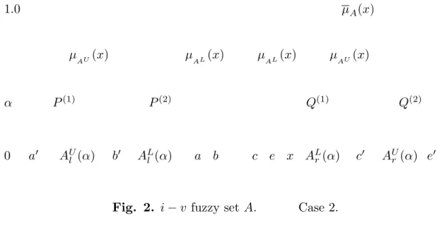
Insert Fig.2 here

In Fig.1, let ρ = λ = 1, and {x | maxµ_AL(x; 1) = 1} = [b, c], {x | maxµ_AU(x; 1) = 1} = [a, e]. Then we obtained the i-v fuzzy set in Fig.2. Let F∗

iv be the family of

these fuzzy sets, then for each 0 ≤ α ≤ 1, the α-cut of A(∈ F∗

iv) in R∗(A) ( the

shaded area in Fig.2 ) is [AU

l (α), ALl (α)] ∪ [ALr(α), AUr(α)] ( see Fig.2 ). Together

with Definition 3 (2◦_{), we have}

d∗(A; 1, 1) = 1 4 Z ₁ 0 [AL_l(α) + AL_r(α) + AU_l (α) + AU_r(α)] dα (6) §3 Discussion.

[A]. Compare with Liou and Wan [10], and [6, 7, 12].

Look at the graph of Fig.1, when ρ = 1, and {x |maxµ_AU(x; 1} = [b, c],

µ_AU(x; 1) is strictly increasing when p ≤ x ≤ b; and µ_AU(x; 1) is strictly de-creasing when c ≤ x ≤ q. Fuzzy number AU _{is the fuzzy number discussed in}

[10]. For A = [AL_{, A}U_{], by Definition 3(1}◦_{) and L’Hopital’s rule , we have}

lim λ→0 1 4λ Z _λ 0 [AU l (α) + ALl (α) + ALr(α) + AUr(α)] dα = lim λ→0 1 4[A U l (λ) + ALl (λ) + ALr(λ) + AUr(λ)] = 1 4[A U l (0) + ALl (0) + ALr(0) + AUr(0)] ≡ I (say)

Thus we can define d∗_{(A; 0, 1) by the following:} d∗(A : 0, 1) ≡ lim λ→0d ∗_{(A; λ, 1)} = I + 1 2 Z ₁ 0 [AU_l (α) + AU_r(α)] dα (7)

The index of optimism α = 1

2 in the total integral value defined in [10] is

I12 T(AU) = 1 2 Z ₁ 0 [AU_l (α) + AU_r(α)] dα (8)

From (7) and (8), the fuzzy numbers in [10] has the following relation with the one we discussed in this paper.

d∗(A; 0, 1) = I + I12

T(AU) (9)

Insert Fig.3 here For example, let

µ_AL(x) =            λ(x−p) q−p , p ≤ x ≤ q λ(r−x) r−q , q ≤ x ≤ r 0, otherwise µ_AU(x) =                    (x−a) b−a , a ≤ x ≤ b 1, b ≤ x ≤ c (d−x) d−c , c ≤ x ≤ d 0, otherwise

where a < p < b < q < c < r < d, 0 < λ < 1 (see Fig.3). Then we have the i-v fuzzy set A = [AL_{, A}U_{]. For each 0 ≤ α ≤ λ, the left and right points of the α -cut of A}L

are AL

right points of the α -cut of AU _{are A}U l (α) = a + (b − a)α, AUl (α) = d − (d − c)α. Therefore I = 1 4(p + r + a + d) I12 T (AU) = 1 2 Z ₁ 0 [a + d + (b − a)α − (d − c)α] dα = 1 4[a + b + c + d], d∗(A; 0.1) = 1 4(p + r + b + c + 2a + 2d)

Look at the graph of µ_AU(x; ρ) in Fig.1. When ρ =sup

x µAU(x; 1) = 1, the fuzzy

number AU _{is the fuzzy number discussed in [12]. The ranking fuzzy number}

dis-cussed in section 3 of [12] has the same result as those disdis-cussed in [6], [7], and the measure, 1₂ R₀1[AU

l (α) + AUr(α)] dα, for the fuzzy set AU in [6], [7], are the same as

the signed distance in [12]. Therefore the fuzzy number in this paper is linked with the one in [6, 7, 12] by (9).

[B] Compare with Yager [11]

In [11], p161, he defined the measure of the fuzzy number B by

F (B) =

Z _αmax

0

M (Bα) dα (10)

where M (Bα) is the mean of the Bα level sets of B. Here A = [AL, AU] is the

i-v fuzzy set in Fig.1. If we only consider the graph of µ_AU(x; ρ), we see AU

is the fuzzy number in [11]. As discussed in [A], by Definition 3(1◦_{), we can}

define d∗_{(A; 0, ρ) by the following:}

d∗(A; 0, ρ) = lim λ→0d ∗_{(A; λ, ρ) = I +} 1 2ρ Z _ρ 0 [AU_l (α) + AU_r(α)] dα (11)

From (10), (11), then we have

d∗_{(A; 0, ρ) = I +} 1 ρF (A

[C]. The signed distance of the level (λ, 1) interval-valued fuzzy number in Fiv ( see

section 2 ).

In section 2, suppose A = [AL_{, A}U_{] is an interval-valued fuzzy set. Here A}L

is not a normal triangular fuzzy number, denoted as AL _{= (a, b, c; λ) and A}U

is a triangular fuzzy number, denoted as AU _{= (p, b, q; 1). The membership}

function of AL _is µ_AL(x) =            λ(x−a) b−a , a ≤ x ≤ b λ(c−x) c−b , b ≤ x ≤ c 0, otherwise

Then we have A = [(a, b, c; λ), (p, b, q; 1)] is called a level (λ, 1) interval-valued fuzzy number. The α-cut (0 < α < 1) of AL _{is A}L

l(α) = a + (b − a)αλ, ALr(α) = c − (c − b)α

λ. The α-cut of AU is AUl (α) = p + (b − p)α, AUr(α) = q − (q − b)α.

From Definition 3 (1◦_{), we have}

d∗(A; λ, 1) = 1

8[6b + a + c + 4p + 4q + 3λ(2b − p − q)] (12) For example, in the inventory problem [13] mentioned in tne Introduction, the total demand during the whole period T is around r0. They were using the

following interval-valued fuzzy set to express it.

µ_rL(x) =            λ(x−r0+∆3) ∆3 , r0− ∆3 ≤ x ≤ r0 λ(r0+∆4−x) ∆4 , r0 ≤ x ≤ r0+ ∆4 0, otherwise µ_rU(x) =            (x−r0+∆1) ∆1 , r0− ∆1 ≤ x ≤ r0 (r0+∆2−x) ∆2 , r0 ≤ x ≤ r0+ ∆2 0, otherwise

where 0 < ∆3 < ∆1 < r0, 0 < ∆4 < ∆2, 0 < λ ≤ 1 (see Fig. 4).

Insert Fig. 4 here

Let r = [rL_{, r}U_{] be this interval-valued fuzzy set. From (12), we have} d∗(r; λ, 1) = 2r0+ 1 8[∆4− ∆3+ (4 − 3λ)(∆2− ∆1)] = 11 + 3λ 8 r0+ 1 8∆4+ 4 − 3λ 8 ∆2+ 1 8(r0− ∆3) + 4 − 3λ 8 (r0− ∆1) Since 4 − 3λ > 0, r0− ∆1 > 0, r0− ∆3 > 0, we have d∗(r; λ, 1) > 0. Let

r∗ = 1 2d

∗_{(r; λ, 1) = r}

0+ 1

16[∆4− ∆3+ (4 − 3λ)(∆2− ∆1)]

This is the estimation of the total demand during the period T in the fuzzy sense. When ∆1 = ∆2, ∆3 = ∆4, then the two triangulars in Fig.4 are isosceles and

r∗ _{= r}

0. That is, the estimation r∗ in the fuzzy sense equals to the crisp value r0.

When ∆1 < ∆2, ∆3 < ∆4, then both the two triangulars in Fig.4 are skew to the

right and r∗ _{> r}

0. When ∆1 > ∆2, ∆3 > ∆4, then both the two triangulars in

Fig.4 are skew to the left and r∗ _{< r}

0. This is a reasonable result as we can see

from Fig.4.

[D]. The signed distance in this paper is an extension of the signed distance on R. For any real number x ∈ R, we can fuzzify x and get a triangular fuzzy number e

x = (x − ∆1, x, x + ∆2; λ), 0 < ∆j, j = 1, 2 and ex is not normal. Also we can

have a level (λ, ρ) interval-valued fuzzy number ex∗ _{= [(x−∆}

1, x, x+∆2; λ), (x−

∆3, x, x + ∆4; ρ)], 0 < ∆1 < ∆3, 0 < ∆2 < ∆4; 0 < λ ≤ ρ ≤ 1. All these are

extension of R.

If ∆1 = ∆2 = ∆3 = ∆4 = 0 and ρ = λ then we have ex = ex∗ = xλ (level λ fuzzy point. i.e. if t = x, µxλ(t) = λ, and if t 6= x, µxλ(t) = 0. ) which

corresponds to x ∈ R. i.e. the level (λ, λ) interval-valued fuzzy numbers ex∗

are all extension points of R. Hence we extend this concept of ranking on R to the ranking of the fuzzy numbers and the ranking of the interval-valued fuzzy sets. Meanwhile we also maintain the properties of the order relation on R. The comparison of the ranking of fuzzy numbers in [ 2, 3, 4, 6, 7 ] with the signed distance ranking of fuzzy numbers in [12] is stated in section 3 of [12]. Also we learn the relation among them through the discussions in [A], [B] in this section.

Acknowledgment I wish to express my deeply thanks for the suggestions to Prof. Emeritus Jing-Shing Yao and also to the referee’s who gave me so many valuable opinions to make this paper done.

References

[1] Sjored M. Baas and Huibert Kwakernaak. Rating and ranking of multiple-aspect alternatives using fuzzy sets. Automatica 13, p. 47-58, 1977.

[2] J.B. Baldwin, N.C.F.Guild. Comparison of fuzzy numbers on the same decision space. Fuzzy sets and systems 2 (1979). 213-233.

[3] S.H. Chen. Ranking fuzzy numbers with maximizing set and minimizimg set. Fuzzy sets and systems 17 (1985) 113-129.

systems 54 (1993) 287-294.

[5] Didier Dubois. Ranking fuzzy numbers in the setting of possibility theory. Information 30, 183-224 (1983).

[6] Phillppe Fortemps, Marc Roubens. Ranking and Defuzzification methods based on area compensation. Fuzzy sets and systems 82 (1996) 319-330. [7] A. Gonzalez . A study of the ranking function approach through mean values.

Fuzzy sets and systems 35 (1990) 29-41.

[8] Antonio Gonzalez. A discrete method for studying indifference and order rela-tions between fuzzy numbers. Information sciences 56, 245- 258, 1991.

[9] Arnold Kaufmann and Madan M. Gupta. Introduction to fuzzy arithmetic. Theory and Applications. Van Nostrand Reinhold. New York 1991.

[10] Tian-Shy Liou and Mao-jiun J. Wan. Ranking fuzzy numbers with integral value. Fuzzy sets and system 50 (1992) 247-255.

[11] R.R. Yager. A procedure for ordering fuzzy subsets of the unit interval. Infor-mation sciences 24 , (1981) 143-161.

[12] Jing-Shing Yao and Kweimei Wu. Ranking fuzzy numbers based on decomposi-tion principle and signed distance. Fuzzy sets and systems 116 (2000) 275-288. [13] Jing-Shing Yao, Jing-Shieh Su. Fuzzy inventory with backorder for fuzzy total demand based on interval-valued fuzzy set. European Journal of Operational Research . 124 (2000) 390-408.

[14] H.J. Zimmermann. Fuzzy set theory and its applications. Second Revised Edition. Kluwer academic publishers. Boston / Dordrecht / London (1991).

1.0 ρ µ_A(x) λ µ_AU(x; ρ) µ_AL(x; λ) µ_AU(x; ρ) α 0 p AU l (α) ALl (α) x ALr(α) AUr(α) q

1.0 µ_A(x)

µ_AU(x) µ_AL(x) µ_AL(x) µ_AU(x)

α P(1) _P(2) _Q(1) _Q(2)

0 a0 _AU

l (α) b0 ALl (α) a b c e x ALr(α) c0 AUr(α) e0

1.0

λ

0 a p b q c r d

1.0

λ

0 r0− ∆1 r0− ∆3 r0 r0+ ∆4 r0+ ∆2