階層式基地台合作技術之效能評估

(1)

國立交通大學

電信工程研究所

碩士論文

階層式基地台合作技術之效能評估

Performance Evaluation of Hierarchical Base

Station Cooperation Techniques

研究生：蔣宗廷

指導教授：王蒞君教授

(2)

階層式基地台合作技術之效能評估

Performance Evaluation of Hierarchical Base

Station Cooperation Techniques

研究生：蔣宗廷

Student：Tsung-Ting Chiang

指導教授：王蒞君 Advisor：Li-Chun Wang

國立交通大學

電信工程研究所

碩士論文

A Thesis

Submitted to Institute of Communications Engineering College of Electrical and Computer Engineering

National Chiao Tung University in partial Fulfillment of the Requirements

for the Degree of Master of Science

In

Communication Engineering September 2011

Hsinchu, Taiwan, Republic of China

(3)

階層式基地台合作技術之效能評估

學生：蔣宗廷

指導教授：王蒞君教授

國立交通大學

電機學院電信工程研究所

摘要

在本篇論文中，我們在第三代合作夥伴計劃-長期演進技術的環

境下，介紹多重輸入多重輸出及階層式基地台合作之模擬平台的建

構方法，並且符合目前第三代合作夥伴計劃的模擬結果。除此之外，

我們同時去分析頻譜使用效率及能源使用效率。據我們所知，目前

文獻上並沒有針對階層式基地台合作，同時評估其頻譜使用效率及

能源使用效率的系統。我們發現，不同的系統在頻譜使用效率及能

源使用效率上會有所取捨。在階層式基地台合作技術下，使用單一

細胞識別可以獲得較佳的能源使用效率，然而，使用多細胞識別則

可以獲得較好的頻譜使用效率。

(4)

Abstract

In this thesis, we discuss the methodology for evaluating the input multi-output (MIMO) systems in the 3rd _{Generation Partnership Project (3GPP)}

Long-Term Evolution-Advanced (LTE-A) environment, and give consistent simulation re-sults with those from the other partners in 3GPP. Moreover, we evaluate the hierarchi-cal base station cooperation (HBSC) systems and give some guidelines for designing the hierarchical cell architectures. Both spectral efficiency (bits/s/Hz) and energy efficiency (bits/J oule) are investigated in our systems. To the best of our knowl-edge, research papers considering both spectral efficiency and energy efficiency for the HBSC systems in the LTE-A environment are rarely seen in the literature. We find some interesting guildline to evaluate the tradeoffs between spectral efficiency and energy efficiency in the HBSC systems. Compared with the single cell ID HBSC system, we obtain a higher spectral efficiency but a lower energy efficiency by adopting the HBSC system with multiple cell IDs.

(5)

Acknowledgments

I especially would like to thank professor Li-Chun Wang who gave me not only many valuable suggestions in the research during these two years but also lots of encour-agements. I would not ﬁnish this work without his guidance and comments.

In addition, I am deeply grateful to my laboratory mates, Dr. Meng-Lin Ku, Dr. Chu-Jung Yeh, Ang-Hsun, Ssu-Han, Yeh-Teng, Yu-Jung, Kai-Ping, Chien-Cheng, Wei-Ping, and junior laboratory mates in Mobile Communications and Cloud Com-puting Laboratory at the Institute of Communications Engineering in National Chiao-Tung University. They always provide me much assistance and share much happiness with me. Special thanks should go to Yi-Ting Lee who gives me great encouragement and cares for me all of my life.

Finally, I am indebted to my parents and younger sister for their kindliness and endless supports.

(6)

III

List of Tables

2.1 Comparison of Our Work and Other Literatures . . . . 7

4.1 Release 9 Two Antenna Ports Codebook . . . 27

4.2 Release 9 Four Antenna Ports Codebook . . . 28

6.1 Simulation Parameters for MIMO systems . . . . 59

6.2 Performance Evaluation Comparison . . . . 60

6.3 Simulation Parameters for RRH Nodes . . . . 61

6.4 Total System Consumed Power per Sector in HBSC-S Systems 62 6.5 Total System Consumed Power per Sector in HBSC-M Systems 62 6.6 Comparison between Energy Eﬃciency and Spectral Eﬃciency (d = 0.6R) . . . . 63

(10)

VII

List of Figures

1.1 Conventional MIMO systems. . . 2

1.2 Network MIMO systems. . . 3

2.1 Frame structure in the downlink and the uplink. . . 10

3.1 SCM parameters of the user and base station. . . 13

3.2 Horizontal antenna pattern for the 3GPP macro-cell. . . 15

3.3 Cell architecture of MIMO systems. . . 17

3.4 Cell architecture of the HBSC-S systesm. . . 18

3.5 Cell architecture of the HBSC-M systesm. . . 20

4.1 Flow chart for the physical layer simulator. . . 26

5.1 Non-cooperation transmission mode in the hierarchical system. . . 39

6.1 Spectral eﬃciency for 2x2 SU-MIMO with diﬀerent codebook selection mechanisms. . . 45

6.2 MIMO downlink normalized user throughput in LTE-A systems. . . . 46

6.3 5% cell-edge spectral eﬃciency of the HBSC-S systems without ICI. . 48

6.4 5% cell-edge spectral eﬃciency of the HBSC-S systems. . . 50

6.5 Cell-average spectral eﬃciency of the HBSC-S systems. . . 50

6.6 Energy eﬃciency of the the HBSC-S systems. . . 52

6.7 5% cell-edge spectral eﬃciency of the HBSC-M systems. . . 54

(11)

6.9 Energy efficiency of the HBSC-M systems. . . 55 6.10 Comparison between energy efficiency and spectral efficiency , d = 0.6R. 57 6.11 Power consumption per sector of HBSC systems for targeting at 2.40

bits/s/Hz. . . 57

(12)

(13)

1

CHAPTER 1 Introduction

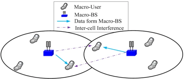
With the rapid growth in the demand for high data rate , the input multi-output (MIMO) antenna system technique is one of the key techniques that can be used to improve radio link throughput [1]. However, because of the cell inter-ference (ICI), the spectral efficiency of MIMO systems at the cell edge is significantly degraded. As shown in Fig. 1.1, if a user is located at the cell edge, it suffers severe inter-cell interference from the neighboring macro cell.

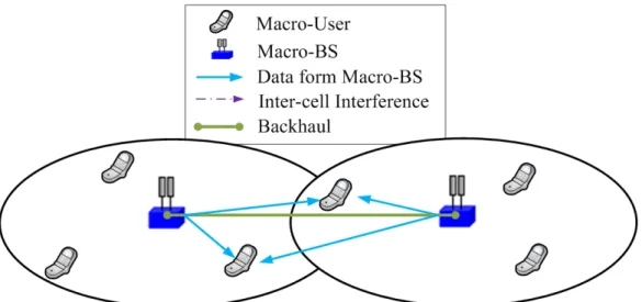
To mitigate the inter-cell interference resulted from the neighboring cells and to enhance the signal-to-interference-plus-noise (SINR) ratio, the concept of joint MIMO processing among cooperative multiple base stations (BSs), referred to net-work MIMO, has recently been proposed [2–6]. Fig. 1.2 illustrates the general idea of the network MIMO system. The cooperative BSs are connected by the high-speed backhaul (e.g. optical ﬁber). With the backhaul, some certain information, i.e. channel state information (CSI) and transmit data, can be interchanged via the backhaul. Hence, the cooperative BSs can jointly work MIMO processing just like a huge virtual-MIMO system. Advanced network MIMO techniques, such as switching between conventional MIMO systems and network MIMO [7], and the combining of frequency partition and network MIMO [8], have been proposed to further enhance the downlink throughput of the network MIMO systems.

(14)

Figure 1.1: Conventional MIMO systems.

used to eliminate ICI in the next-generation wireless systems, such as the IEEE 802.16m Worldwide Interoperability for Microwave Access (WiMAX) standard and the Third Generation Partnership Project (3GPP) Long-Term Evolution-Advanced (LTE-A) standard. In IEEE 802.16m WiMAX, there are two scenarios for multi-BS processing (1) closed-loop marco diversity (CL-MD) and (2) collaborative MIMO (Co-MIMO) transmission. To apply CL-MD transmission, a single user is served jointly by multiple cooperative BSs. To apply the Co-MIMO transmission, several users are served jointly by multiple cooperative BSs [9]. A similar concept is proposed in the LTE-A standard, called coordinated multi-point (CoMP) transmission. There are three scenarios (1) coordinated scheduling/coordinated beamforming (CS/CB), (2) single-user (SU) joint processing (JP) (corresponding to CL-MD in WiMAX), and (3) multi-user (MU) JP (corresponding to Co-MIMO in WiMAX). CS/CB is another technique that several BSs are coordinated to schedule users and search the suitable beamforming matrix for each user [10–13]. The data is transmitted only from the single BS. These approaches are worse than the JP techniques but reduce the amount of exchanging data via the backhaul. Single-user-JP-CoMP is similar to

(15)

Figure 1.2: Network MIMO systems.

CL-MD where multiple BSs jointly serve a single user. Both multi-user-JP-CoMP and Co-MIMO transmissions allow multiple coordinated BSs to serve multiple users simultaneously with jointly designed precoding matrix.

1.1 Problem and Solution

Network MIMO is one of the potential techniques for a next-generation wireless sys-tem to eliminate ICI and enhance the cell-edge spectral eﬃciency. Generally, neigh-boring cells in a network MIMO system are linked by a high-speed backhaul to ex-change users’ information. Hence, several BSs can cooperate to provide joint MIMO signal processing. However, cooperating at the large-cell level (e.g. macro-cell) re-sults in higher cost and more complex system design. This is because the distance between cooperative BSs is too long. The cost of the backhaul connection and the synchronization issues are crucial. In [14], it was shown that the performance of the network MIMO system degrades signiﬁcantly when considering the large feedback

(16)

delay. Hence, we do not cooperate cells in a large area. On the contrast, we place some low power BSs, e.g. RRH nodes, at the edges of macro-cells and cooperate these nodes in a smaller area.

Moreover, we consider two different RRH types (1) RRH nodes that share the same cell ID with the corresponding macro-BS and, (2) RRH nodes for which each RRH node has an individual cell ID that is different from the corresponding macro-BS. These two types of RRH nodes result in a difference in performance. In (1), the macro-BS and the RRH nodes with the same cell ID are cooperated, and we refer to the system as Hierarchical Base Station Cooperation with the Single cell ID (HBSC-S). In (2), the macro-BS and the RRH nodes with the different cell IDs are cooperated, and we refer to the system as Hierarchical Base Station Cooperation with Multiple cell IDs (HBSC-M). Generally, the HBSC-S system is simple but has lower spectral efficiency, whereas the HBSC-M system is complex but has higher spectral efficiency.

We evaluate both HBSC-S and HBSC-M systems as well as conventional MIMO systems in an LTE-A environment. The performance of the conventional MIMO system is demonstrated and compared with the existing results in 3GPP. Then, we analyze both spectral efficiency and energy efficiency of the cooperation systems, and illustrate the tradeoffs between spectral efficiency and energy efficiency.

1.2 Thesis Outline

The rest of this thesis is organized as follows. The background of our work is in-troduced in Chapter 2. The overall system models are described in Chapter 3. In Chapter 4, we disscuss the simulation methodology of MIMO systems in the LTE-A environment. Chapter 5 discusses the detailed HBSC system. Subsequently, numer-ical results are shown in Chapter 6. Finally, we conclude this thesis and discuss

(17)

potential future works in Chapter 7.

(18)

6

CHAPTER 2 Background

2.1 Literature Survey

Many researchers have investigated several cooperation schemes. In [3], they provided both the theoretic upper-bound and some practical schemes in the downlink coopera-tion systems. The upper bound was obtained by implementing the dirty paper coding (DPC). In [4], the singular value decomposition (SVD) based network MIMO scheme with various antenna number was investigated. They concluded that cooperating among several cells can bring the enormous gain in the spectral efficiency and showed that the capacity increases as the antenna number increases. In [6], the performance of cooperation among various cell number was discussed. The author concluded that the throughput can be improved if the number of cooperative cells or the number of sectors per cell increases. However, [3,4,6] only cooperated BSs at the large-cell level, and do not take into account of feedback accuracy. Moreover, they only considered the spectral efficiency rather then energy efficiency.

In [15], they illustrated the BS deployment strategies under cellular networks from the energy eﬃciency aspects. It placed some low-power nodes in the macro-cell to enhance the cell-edge throughput. Moreover, they introduce two concepts, i.e., the area power consumption and the area spectral eﬃciency. The area power con-sumption is used to estimate the total power concon-sumption relative to the coverage

(19)

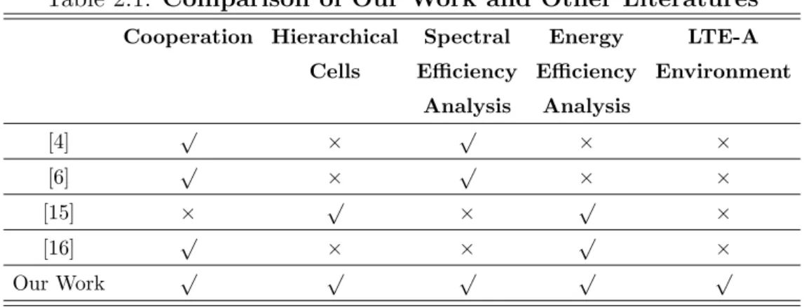
Table 2.1: Comparison of Our Work and Other Literatures

Cooperation Hierarchical Spectral Energy LTE-A Cells Eﬃciency Eﬃciency Environment

Analysis Analysis [4] √ × √ × × [6] √ × √ × × [15] × √ × √ × [16] √ × × √ × Our Work √ √ √ √ √

in Watts per square kilometers, and the area spectral efficiency is used to estimate the spectral efficiency relative to the coverage in bits per second per Hertz per square kilometers. The performance with the various number of low-power nodes was also investigated. However, they did not deal with the extra intra-cell interference caused by the low-power nodes. In [16], the author demonstrated the additional consumed power including signal processing power, backhaul power, and pilots power. They also consider the signalling overhead including pilots and CSI feedback. With the vari-ous cell sizes and cooperation sizes, the author indicated that cooperating more than three macro-cells is not energy-efficient. However, only one BS type, i.e., macro-cell, was considered. We compare our work with the above research in Table 2.1. We in-vestigate both spectral efficiency and energy efficiency in our hierarchical cooperation systems. Moreover, we evaluate the systems in the LTE-A environment.

2.2 3GPP LTE-A Systems

The 3rd _{Generation Partnership Project (3GPP) has adopted orthogonal frequency}

division multiple access (OFDMA) in the downlink and single carrier frequency divi-sion multiple access (SC-FDMA) in the uplink of LTE-A systems. The advantages

(20)

of using OFDMA in the downlink include not only overcoming the multipath prob-lem, but also making use of the adaptive modulation and coding schemes (MCS). On the other hand, the advantage of using SC-FDMA is the ability to reduce the peak-to-average power ratio (PAPR).

To achieve the target downlink peak spectral efficiency of 30 bits/s/Hz and up-link peak spectral efficiency of 15 bits/s/Hz [17], many techniques have been suggested for the 3GPP LTE-A systems, including SU-MIMO, MU-MIMO, relaying techniques, carrier aggregation (CA), enhanced inter-cell interference coordination (eICIC), and CoMP. SU-MIMO is a common technique to improve radio link throughput in 3GPP LTE-A systems. It utilizes transmit diversity or multiple spatial layers to transmit the data to a single user equipment (UE). Several transmission modes are adopted, e.g. transmit diversity, open-loop spatial multiplexing, closed-loop spatial multiplex-ing, beamformmultiplex-ing, etc. In MU-MIMO systems, the BS serves multiple users in the same time-frequency resource by making use of degrees of freedom (DoF) in the spatial domain. It enhances the cell-average spectral efficiency as compared to SU-MIMO systems. Relay nodes are connected with the BS wirelessly and help further serve the cell-edge users. CA is used to collect several discontinuous frequency bands and hence we can utilize a larger bandwidth up to 100 MHz. CoMP and eICIC are two techniques used to control the inter-cell interference, where the former uses the cooperation among certain BSs and the latter takes advantage of radio resource management (RRM).

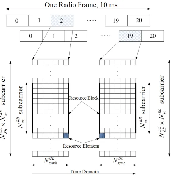
In order to catch on the detailed time-frequency resource used in LTE-A sys-tems, we need to understand the physical resource block (RB) deﬁned in [18]. One radio frame with 10 milliseconds consists of 20 time slots. Each time slots can divided into NU L

RB resource blocks (RBs) and NRBDL RBs for the uplink and downlink

respec-tively. In the frequency domain, both the uplink RB and the downlink RB consist of NRB

(21)

symbols and one downlink RB consists of N_symbDL OFDM symbols. Hence, one uplink RB consists of NRB

sc × NsymbU L resource elements (REs) and one downlink RB consists

of N_scRB× N_symbDL REs. We show the frame structure in Fig. 2.1.

2.3 LTE-A System-Level Simulator

For the purpose of evaluating the performance and proposing practicable schemes under the LTE-A standard, it is necessary to build the LTE-A simulator. To our knowledge, many equipment vendors and some research centers have already con-structed their own simulators, but rarely describe their simulation methodology. In [19] and [20], they built a LTE-A simulation platform but did not compare their results with LTE-A calibration results. We have shown the calibration results com-pared with [21–23] in our lab (Mobile Communication and Cloud Computing Lab, Institute of Communications Engineering, National Chiao-Tung University) [24]. By examining the two steps (step (1a) for wideband SINR and step (1c) for spectral eﬃciency) performance metrics deﬁned in [22], our lab’s work is consistent with other existing simulation calibration results.

(22)

(23)

11

CHAPTER 3 System Models

In this chapter, we introduce our system models in detail. Three cellular system models are described in the ﬁrst three sections, i.e., cellular MIMO systems, hier-archical hierhier-archical BS cooperation with single cell ID (HBSC-S), and hierhier-archical BS cooperation with multiple cell IDs (HBSC-M). In the last section, we discuss the energy consumption issues and give reasonable models for each cellular system.

3.1 Channel Model

A suitable propagation channel model is important for numerical analysis. It models how the transmit signals propagate through the air space. Thus, we follow the channel model to characterize radio eﬀects in the 3GPP LTE-A environment [22] and introduce each parameter in the following section.

3.1.1 Spatial Channel Model

The spatial channel model (SCM) is widely used in LTE-A systems simulation [25, 26]. In the early years, the International Telecommunication Union Radiocommu-nication Sector (ITU-R) channel model was developed for the International Mobile Telecommunications-2000 (IMT-2000) systems. However, the ITU-R channel model is not well-deﬁned due to the renewed parameters, such as bandwidth, frequency

(24)

band. Moreover, the ITU-R model is not suitable for the MIMO systems since it does not model the spatial correlation between antennas. Hence, SCM has been de-veloped to model the channel more correctly. As we know, SCM characterizes the spatial correlations as well as the multi-path fading. In the following, we discuss the formulations and parameters of SCM brieﬂy.

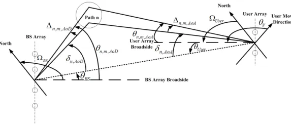
The urban-macro scenario is adopted in our SCM simulations [22]. The macro-cell usually serves a large area, and hence the probability of experiencing a line-of-sight (LOS) environment tends to zero. Therefore, the LOS component can be neglected. Assume that there are N paths with each consisting of M subpaths in each link from the BS to the user. We introduce each parameter in Fig. 3.1:

θBS : the angle between the LOS and the BS array broadside.

θU ser : the angle between the LOS and the user array broadside.

δn,AoD : the angle between the LOS and the nth (n = 0, 1, 2, ..., N − 1) path.

δn,AoA : the angle between the LOS and the nth (n = 0, 1, 2, ..., N − 1) path.

∆n,m,AoD : the oﬀset of the mth (m = 0, 1, 2, ..., M − 1) subpath within the nth path

relative to δn,AoD.

∆n,m,AoD : the oﬀset of the mth (m = 0, 1, 2, ..., M − 1) subpath within the nth path

relative to δn,AoA.

θV : the angle between the user movement direction and the user array broadside.

θn,m,AoA : θn,m,AoA = θU ser+ δn,AoA + ∆n,m,AoA.

θn,m,AoD : θn,m,AoA = θBS+ δn,AoD+ ∆n,m,AoD.

(25)

Figure 3.1: SCM parameters of the user and base station. formulate the channel response matrix hn(t)∈ CNr×Nt _as

hn(t) =         h1,1,n_(t) _h1,2,n_(t) _{· · · h}1,Nt,n_(t) h2,1,n_(t) _h2,2,n_(t) · · · h2,Nt,n_(t) .. . ... · · · ... hNr,1,n_{(t) h}Nr,2,n_(t) · · · hNr,Nt,n_(t)         . (3.1)

Each element in hn(t) can be written as :

hu,s,n(t) = √ Pn M M ∑ m=1 (

ejkdssin(θn,m,AoD+ψn,m)_ejkdusin(θn,m,AoA)_ejkV cos(θn,m,AoA−θV)t) _,

(3.2) where Pnis the power of the nth path, θn,m,AoD is the angle between the mth subpath

within the nth path and the BS array broadside, θn,m,AoA is the angle between the

mth _{subpath within the n}th _{path and the user array broadside, M is the number of}

subpaths per path, k is the carrier wavelength in meters, ds is the distance from the

ﬁrst antenna to the sth _{antenna at the BS in meters, d}

u is the distance from the ﬁrst

antenna to the uth_{antenna at the user in meters, ψ}

n,m is the phase of the mthsubpath

within the nth path with uniform distribution in the interval [0◦, 360◦], V is the user 13

(26)

speed, and θV is the angle between the user movement direction and the user array

broadside.

Note that (3.1) is deﬁned in the time domain. In order to apply the OFDM system, we must transform the time domain channel response into frequency do-main. Let NF F T denote the fast Fourier transform (FFT) size. The SCM for the kth

subcarrier in the frequency domain can be formulated as

HSCM(k) =         H1,1_(k) _H1,2_(k) _{· · · H}1,Nt_(k) h2,1_(k) _H2,2_(k) · · · H2,Nt_(k) .. . ... · · · ... HNr,1_{(k) H}Nr,2_(k) · · · HNr,Nt_(k)         , k = 1, 2, ..., NF F T . (3.3)

Each element of H(k) can be written as

Hu,s(k) = F F T [hu,s,1(t), hu,s,1(t), ..., hu,s,N(t)] , (3.4) where Hu,s_{(k) denotes the channel response coeﬃcient from the s}th _{transmit antenna}

to the uth receive antenna in the kth subcarrier, F F T denotes the FFT function with size NF F T, and hu,s,n(t) was shown in (3.2).

3.1.2 Radio Environments

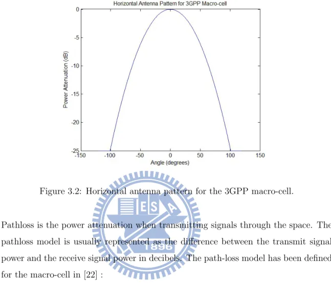
Directional antenna pattern, path-loss model, and shadowing model are considered in our radio environment. A horizontal antenna pattern is deﬁned for each ﬁxed sector in 3GPP LTE-A systems [22]. It can be shown as

AdB_s,b,u(ϕ) =− min [ 12 ( ϕs,b,u ϕ3dB )2 , Am ] , (3.5)

where ϕs,b,u is the angle between the beam direction of the sth BS and the uth user

in the bth _{sector, ϕ}

3dB is 70 degrees, and Am is 25 dB. Note that ϕ3dB denotes the

(27)

Figure 3.2: Horizontal antenna pattern for the 3GPP macro-cell.

Pathloss is the power attenuation when transmitting signals through the space. The pathloss model is usually represented as the diﬀerence between the transmit signal power and the receive signal power in decibels. The path-loss model has been deﬁned for the macro-cell in [22] :

P LdB_s,b,u = 128.1 + 37.6log₁₀(ds,b,u), (3.6)

where P LdB_s,b,u is the power-loss term between the sth BS and the uth user in the

bth _{sector, and d is the distance from the s}th _{BS to the u}th _{user in the b}th _sector

in kilometers. The shadowing eﬀect is caused by obstacles. It is modeled by the log-normal distribution with zero mean and 8 dB standard deviation.

For simplicity, we describe our following channel model in the single-carrier case. It can be extended to the multi-carrier case in the same way. Let Hs,b,u ∈ CNr×Nt

denote the overall channel response including the spatial channel model and radio

(28)

eﬀects. Thus, we can derive the overall complex baseband channel response as

Hs,b,u= HSCM

√

ηs,b,uAs,b,u(P Ls,b,u)−1 , (3.7)

where Hs,b,u is the channel response from the sth BS to the uth user in the bth sector,

HSCM ∈ CNr×Nt _{is the SCM matrix shown in (3.3), η}

s,b,uis the log-normal distribution

shadowing with zero mean and 8 dB standard deviation, As,b,u = 10(A

dB

s,b,u/10), and

P Ls,b,u= 10(P L

dB s,b,u/10).

3.2 Cellular MIMO Systems

The cellular system consists of 19 cell cites with hexagonal grid as shown in Fig. 3.3. Each hexagonal grid macro-cell is divided into three sectors, where each sector is equipped with directional antennas. Recall that there are Nt transmit antennas

at each BS, Nr receive antennas at each user, and total Nu users in each sector.

Denote Hs,b,u ∈ CNr×Nt as the channel matrix from the sth BS to the uth user in the

bth _{sector, X}

b,u as the desired signal of the uth user in the bth sector, and Wb,u as

the corresponding weighting matrix for the uth user in the bth sector, respectively. Generally, the receive signal can be modeled as follows

Yb,u = H_| b,b,uW_{zb,uXb,u_}

desired signal

+∑

m̸=b

Hm,b,uWm,nXm,n

| {z }

inter−cell interference

+nb,u , (3.8)

where nb,u ∈ CNr×1 is the additive white noise with σn2 = −174 dBm/Hz power

density.

3.3 Hierarchical Base Station Cooperation Systems

In this section, we discuss the models of HBSC systems. Several RRH nodes are ﬁxed in each macro-cell and each RRH node is connected to the macro-BS by the backcaul

(29)

Figure 3.3: Cell architecture of MIMO systems.

(e.g. optical ﬁber). Hence, the desired information (e.g. CSI, transmit data) can be exchanged rapidly between the macro-BS and RRH nodes.

Two different RRH node types are considered (1) the RRH nodes share the same cell ID with the corresponding macro-BS, and (2) each RRH node has the in-dividual cell IDs different from the corresponding macro-BS. In the former case, the macro-BS and the RRH nodes share the same single cell ID and cooperate with each other. We can regard RRH nodes as the distributed antennas within the correspond-ing macro-BS. In the latter case, the macro-BS and the RRH nodes with the different cell IDs are cooperated. Since each RRH node has a unique cell ID, we can regard these RRH nodes as individual low-power BSs. Each RRH node can serve their own users just as macro-BS do. There are multiple cell IDs in a cooperative set.

3.3.1 Cooperation with Single Cell ID

Based on [27], NH = 4 RRH nodes ﬁxed in every sector are regarded as the baseline

and is shown in Fig. 3.4. Note that the distances between neighboring RRH nodes

(30)

Figure 3.4: Cell architecture of the HBSC-S systesm. are equal in our assumptions.

Since the RRH nodes share the same cell ID with the corresponding macro-BS in the Hmacro-BSC-S systems, the reference signals are placed at the same resource elements (REs) and sent by the macro-BS and each RRH nodes simultaneously [28]. Let HRRH_s_r_,b,u ∈ CNr×Nt _{denote the channel matrix from the r}th _{RRH node in the s}th

sector to the uth _{user in the b}th _{sector. The u}th _{user in the b}th _{sector can only detect}

the eﬀective channel Hef f_b,b,u ∈ CNr×Nt_{, where} Hef f_b,b,u = Hb,b,u+

∑

r

HRRH_b_r_,b,u . (3.9) Hence, the receive signal of the uth _{user in the b}th _{sector can be modeled as}

Yb,u = H ef f

b,b,uWb,uXb,u

| {z } desired signal +∑ m̸=b Hef f_m,b,uWm,nXm,n | {z }

+nb,u , (3.10)

where Xb,u denotes the desired signal of the uth user in the bth sector, Wb,u denotes

the corresponding weighting matrix of the uth _{user in the b}th _{sector, and n}

b,u ∈ CNr×1

(31)

3.3.2 Cooperation with Multiple Cell IDs

We also ﬁx NH = 4 RRH nodes in each sector as the baseline. In the HBSC-M system,

each RRH node can be regarded as an individual low-power BS within the macro-cell coverage. Hence, the RRH nodes can serve its own users just as a macro-BS do. For simplicity, we call users served by the the RRH node as RRH-users, and those by macro-BS as macro-users, respectively.

However, the macro-users and RRH-users suﬀer extra intra-cell interference from the RRH nodes and macro-BS, respectively. Assume that the tth _{user is served}

by the rth _{RRH node and the u}th_{user is served by the b}th _{macro-BS. Denote H}RRH sr,b,t ∈

CNr×Nt _{as the channel from the r}th_{RRH nodes in the s}th_{sector to the t}th _{RRH-user in}

the bth _{sector, X}RRH

br,t as the desired signal of the t

th _{RRH-user served by the r}th _RRH

node in the bth sector, and WRRH_b_r_,t as the corresponding weighting matrix. Hence, we can model the receive signal YRRH_b_r_,t for the tth _{user as}

YRRH_b_r_,t = HRRH_b_r_,b,tWRRH_b_r_,t XRRH_b_r_,t | {z } desired signal + ∑ m Hm,b,tWm,nXm,n | {z }

interference from macro−BSs

+∑ m̸=b HRRH_m k,b,tW RRH mk,b,tX RRH mk,b,t | {z }

interference from RRH nodes

+nRRH_b_r_,t , (3.11)

where nRRH

br,t is the additive white noise with σ

2

n =−174 dBm/Hz power density. Note

that the second term in right hand side of (3.11) is the inter-cell interference from the all the macro-BSs, and the third term in the right hand side of (3.11) is the inter-cell interference from the RRH nodes in the other macro-cell.

Similarly, the received signal Yb,u ∈ CNr×1 of the uth user served by the bth

sector can be modeled as

Yb,u = H_| b,b,uW_{zb,uXb,u_}

desired signal

+ ∑

m̸=b

Hm,b,uWm,nXm,n

| {z }

interference from macro−BSs

(32)

Figure 3.5: Cell architecture of the HBSC-M systesm. +∑ m HRRH_m k,b,uW RRH mk,b,uX RRH mk,b,u | {z }

interference from RRH nodes

+nb,b,u , (3.12)

where nbr,u is the additive white noise with σ

2

n=−174 dBm/Hz power density. Note

that the second term in the right hand side of (3.12) is the inter-cell interference from other macro-BSs, and the third term in the right hand side of (3.12) is the inter-cell interference from all the RRH nodes in each macro-cell.

If the RRH-user and the macro-user are served by the corresponding BSs simultaneously and each user is not very close to their serving BS, strong intra-cell interference will degrade the spectral eﬃciency of both RRH-user and macro-user. We apply the network MIMO technique to overcome this problem. As shown in Fig. 3.5, the macro-BS and the RRH node are connected via a high speed backhaul, and work like a virtual MIMO system to jointly serve both the macro-user and RRH-user. We denote the distance between the macro-BS and each RRH node as d and the cell radius as R. Note that the distance between each neighboring RRH node is equal.

(33)

macro-BS in the bth sector are co-scheduled to apply network MIMO. Note that each RRH node shares diﬀerent cell IDs with the macro-BS so that the tth _{RRH-user can}

detect the channel come from the RRH node (HRRH_b_r_,b,t), and the other channel coming from the macro-BS (Hb,b,t). Similarly, the uth macro-user can detect the channel

coming from the macro-BS (Hb,b,u), and the other channel coming from the RRH

node (HRRH_b_r_,b,u). If we regard these coordinated nodes as a virtual MIMO system, a combined channel matrix of the co-scheduled users can be respectively written as

Hcom_b,b,t and Hcom_b,b,u, where

Hcom_b,b,t = [ HRRH_b_r_,b,t Hb,b,t ] , (3.13) and Hcom_b,b,u = [ HRRH_b_r_,b,u Hb,b,u ] . (3.14) Hence, we can rewrite the receive signal Yb,t of the tth RRH-user in the bth

sector as

Yb,t= Hcomb,b,tWb,tXb,t

| {z }

desired signal

+ Hcom_b,b,tWb,uXb,u

| {z }

inter−user interference

+∑ m̸=b ( Hcom_m,b,tWm,nXm,n + Hcomm,b,tWm,kXm,k ) | {z }

+nb,t , (3.15)

where Xb,tis the desired signal of the tthRRH-user, Wb,tis the corresponding

weight-ing matrix, and nb,t is the additive white noise with σ2n = −174 dBm/Hz power

density. Note that the second term in the right hand side of (3.15) is the inter-user interference, and the third term in the right hand side of (3.15) is the interference from other cooperative sets. Similarly, we can write the receive signal Yb,u of the uth

(34)

macro-user in the bth sector as

Yb,u = Hcomb,b,uWb,uXb,u

| {z }

desired signal

+ Hcom_b,b,uWb,tXb,t

| {z }

inter−user interference

+∑

m̸=b

(

Hcom_m,b,uWm,nXm,n+ Hcomm,b,uWm,kXm,k

)

| {z }

+nb,u , (3.16)

where Xb,u is the desired signal of the uth macro-user, Wb,u is the corresponding

weighting matrix, and nb,u is the additive white noise with σn2 = −174 dBm/Hz

power density. Note that the second term in the right hand side of (3.16) is the inter-user interference, and the third term in the right hand side of (3.16) is the interference from other cooperative sets.

3.4 Power Consumption Model

In order to further discuss the energy-efficiency issues, a suitable model for power consumptions is important. We have discussed three different nodes in the previous sections, i.e. the macro-BS, the RRH node with the same cell ID as the macro-BS, and the RRH node with different cell IDs from the macro-BS. Thus, we consider three different power models for each node.

Generally, the total power consumed at each BS can be divided into several parts [29]. Denoting Ptotal as the total power consumed at the BS, we can model the

total consumed power per BS as

Ptotal= Nt× ( PT x µpa + Psp ) × βc× βp+ Pbh , (3.17)

where Nt denotes the number of transmit antennas, µpa denotes the power ampliﬁer

eﬃciency, Psp denotes the power used for signal processing, βc denotes the additional

(35)

supply loss, and Pbh denotes the consumed power for exchanging the data via the

backhaul. Note that µpa ≤ 1, βc≥ 1, and βp ≥ 1.

We set the values of each parameter based on [16, 29, 30]. Power amplifiers in the macro-BS usually have better efficiency than those in the RRH nodes due to the worse hardware components in the small BSs. A various power amplifier efficiency 38% and 20% are set for the macro-BSs and RRH nodes respectively. Pspis consumed

by the signal processing and Psp = 58 (Watts) is assumed. βc = 1.29 and βp = 1.11

model the additional power consumed for cooling and power supply loss, respectively. Note that the cooling power is not counted in RRH nodes because small BSs are not equipped with the cooling facilities. Furthermore, Pbh is modeled as

Pbh =

Cbh

100M bits/s × 50 (W atts) . (3.18) where Cbh is the data rate, which is transmitted via the backhaul. It means that if

we transmit the data with the rate 100M bits/s, the consumed power is 50 (Watts). After we have the total consumed power per BS, we formulate the energy efficiency metric. The bits per Joule (bits/J oule) metric is first introduced in [31], and widely used to estimate if the system is energy efficient [16, 29, 30, 32]. Let Ctotal

denote the total throughput (bits/s) in the system so that the bits per Joule metric

Etotal can be written as

Etotal(bits/J oule) =

Ctotal(bits/s)

Ptotal(J oule/s)

. (3.19) Based on the energy eﬃciency metric Etotal, we can estimate how many bits can be

transmitted when consuming one Joule energy in different systems. Therefore, we evaluate the energy efficiency metrics of various systems, and show whether they are energy efficient or not.

(36)

24

CHAPTER 4 MIMO Physical Layer Simulation

Platform

In this chapter, we discuss the procedures for evaluating the SU/MU-MIMO sys-tem level performance in the 3rd _{Generation Partnership Project (3GPP) Long-Term}

Evolution Advanced (LTE-A) environment. To guarantee that the simulation results from various 3GPP partners are comparable, certain assumptions and constraints were agreed in the 3GPP Technical Specification Group (TSG) Radio Access Net-work (RAN) 1 meeting. Many equipment vendors have presented the consistent system level performance calibration results. However, they only provided the simu-lation results without including the detailed simusimu-lation procedures. Hence, we built a LTE-A SU/MU-MIMO system level simulation platform and provide the flow chart for the simulation procedures in the physical layer. Finally, we compare the cell-average spectral efficiency as well as the cell-edge performance with other existing evaluation results.

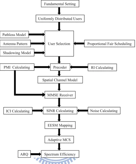
The simulation procedures are described as follows. In the beginning, we drop users uniformly into the entire macro-cell and calculate the radio eﬀects, including the path-loss, shadowing, and antenna pattern. We then generate an urban macro spatial channel model (SCM) for each user. The serving sector for each user is selected based on the maximal reference signal received power (RSRP). That is, each user is given the serving sector that yields the maximal RSRP. In MIMO systems, each user selects

(37)

a precoding matrix indicator (PMI) and a rank indicator (RI) [33], and then feedback them to the BS. PMI is used to determine the precoding matrix, while RI is used to determine the transmission rank. At the receiver, the maximum ratio combining (MRC) and the minimum mean square error (MMSE) algorithms are adopted to demodulate the received signal. We calculate the received signal power and the inter-cell interference in the next step, after which we can derive the SINR for each subcarrier. The best modulation and coding schemes are changed adaptively based on the current channel quality indicator (CQI). Finally, we calculate the spectrum eﬃciency while taking into account retransmission and the downlink overhead. Figure 4.1 shows a ﬂow chart of the simulation procedures.

4.1 Codebook-based Precoder

To ﬁt the LTE-A MIMO system, we apply the codebook-based precoder in our sim-ulation. In the ideal closed-loop MIMO system, each BS calculates the precoding matrix based on the current CSI by assuming that the full CSI is available at the BS. However, it is impractical for each user to feedback the full CSI because the feedback channel bandwidth is limited. In LTE-A MIMO systems, each user calculates the pre-coding matrix and feeds the PMI back as an index of the codebook. The codebook is designed oﬄine, and the same codebook set exists at both the transmitter and the receiver. If users only feed the index back rather than the full precoding matirx, the feedback overhead can be sharply reduced.

The codebooks for two antenna ports and four antenna ports are deﬁned in [34]. The codebook for two transmit antenna ports is given in Table 4.1. Because both rank-1 and rank-2 transmission schemes can be adopted for two transmit antenna ports, two kinds of codebook sets are needed. For rank-1 transmission, four code-words, i.e., C0,C1,...,C3, can be selected from the rank-1 codebook set. Similarly, for

(38)

Figure 4.1: Flow chart for the physical layer simulator.

rank-2 transmission, two codewords, i.e. C0 and C1, can be selected from the rank-2

codebook set.

The codebook for four transmit antenna ports is given in Table 4.2. Sixteen codewords, i.e. C0, C1, ..., C15, can be selected from the rank-1 or the rank-2 codebook

set. Note that the householder matrix Wc is generated by uc, i.e., Wc = I4 −

2ucuHc

/

uH_c uc. Note that Wac denotes the ath column vector of Wc, and Wa,bc denotes

the ath _{and b}th _{column vectors of W}

(39)

Table 4.1: Release 9 Two Antenna Ports Codebook

Index Rnak-1 Rnak-2

C0 √1₂    1 1    1 2    1 1 1 −1    C1 √1₂    1 −1    1 2    1 1 j −j    C2 √1₂    1 j    C3 √1₂    1 −j   

in the codebook sets is normalized to unity because we have to preserve the same transmit power.

The precoder is calculated based on the estimated CSI at the user side. We assume that each user can perfectly estimate the CSI based on the reference signal. Hence, Hb,b,u is known at the uthuser in the bth sector. Based on [35,36], we calculate

the full precoding matrix by using the dominant eigen modes. In the case of Nt≥ Nr,

we ﬁrst decompose the channel Hb,b,u of the uth user in the bth sector by the using

singular value decomposition (SVD) method as follows

Hb,b,u = Ub,b,uSb,b,uVHb,b,u , (4.1)

where Ub,b,u = [ u1_b,b,u · · · uNr b,b,u ] ∈ CNr×Nr _, _(4.2) 27

(40)

Table 4.2: Release 9 Four Antenna Ports Codebook

Index uc Rank-1 Rank-2

C0 u0 = [ 1 −1 −1 −1 ]T W1₀ W1,4₀ /√2 C1 u1 = [ 1 −j 1 j ]T W1₁ W1,4₁ /√2 C2 u2 = [ 1 1 −1 1 ]T W1₂ W1,4₂ /√2 C3 u3 = [ 1 j 1 −j ]T W1₃ W1,2₃ /√2 C4 u4 = [ 1 (−1 − j)/√2 −j (1 − j)/√2 ]T W1₄ W1,4₄ /√2 C5 u5 = [ 1 (1− j)/√2 j (1− j)/√2 ]T W1₅ W1,4₅ /√2 C6 u6 = [ 1 (1 + j)/√2 −j (−1 + j)/√2 ]T W1₆ W1,3₆ /√2 C7 u7 = [ 1 (−1 + j)/√2 j (1 + j)/√2 ]T W1₇ W1,3₇ /√2 C8 u8 = [ 1 −1 1 1 ]T W1₈ W1,2₈ /√2 C9 u9 = [ 1 −j −1 −j ]T W1₉ W1,4₉ /√2 C10 u10= [ 1 1 1 −1 ]T W1₁₀ W1,3₁₀/√2 C11 u11 = [ 1 j −1 j ]T W1₁₁ W1,3₁₁/√2 C12 u12= [ 1 −1 −1 1 ]T W1₁₂ W1,2₁₂/√2 C13 u13= [ 1 −1 1 1− ]T W1₁₃ W1,3₁₃/√2 C14 u14= [ 1 1 −1 −1 ]T W1₁₄ W1,3₁₄/√2 C15 u15= [ 1 1 1 1 ]T W1₁₅ W1,2₁₅/√2

(41)

Sb,b,u =         σ1 b,b,u 0 0 0 0 · · · 0 0 . .. 0 0 0 · · · 0 .. . . .. ... 0 ... . .. ... 0 · · · 0 σNr b,b,u 0 · · · 0         ∈ CNr×Nt _, _(4.3) and VH_b,b,u = [ v1 b,b,u · · · v Nt b,b,u ]H ∈ CNt×Nt _. _(4.4)

Note that σ1_b,b,u ≥ σ_b,b,u2 ≥...≥ σNr

b,b,u. If Ns data streams are transmitted to the uth

user simultaneously, the Ns leftmost column vectors of Vb,b,u are selected as the full

precoding matirx, i.e., fWb,u. Thus, we can transmit the signal on the channel with

a better channel quality. For example, in the SU-MIMO rank-1 system with Nt = 2

and Nr = 2, we select v1b,b,u as the full precoding vector fWb,b,u, where fWb,u is the

percoding vector of the uth user in the bth sector. Similarly, in the SU-MIMO rank-2 system with Nt= 2 and Nr = 2, we select both v1b,b,u and v2b,b,u as the full precoding

matrix fWb,u, where fWb,b,u is the percoding matrix of the uth user in the bth sector.

Once we have the full precoding matrix fWb,u, we search for the most suitable

codeword to represent it since it is impractical for the user feedbacking the full pre-coding matrix with inﬁnite bits. Codewords are selected based on the minimum angle between each codeword and the full precoding matrix [37, 38]

a = arg max i trace (_CH i Wfb,u ) , (4.5)

where Ci is the codeword deﬁned in Tables 4.1 and 4.2, and a is the selected codeword

index. Each user only feeds the index a of the corresponding codeword back. Hence, the number of feedback bits can be sharply reduced.

(42)

4.2 Receiver Structure

At the user, the MRC and MMSE receiver structures are adopted [22, 39]. The MRC receiver is used to maximize the desired receive signal power in the rank-1 SU-MIMO system, whereas the MMSE receiver is used to suppress the stream and inter-user interference in the multi-rank MIMO system, where the former is caused by the multi-stream interference in SU-MIMO systems and the latter is caused by the multi-user interference in MU-MIMO systems.

In the rank-1 SU-MIMO system, the MRC receiver is adopted. Let the uth_user

be the serving user with only one data symbol Xb,u = x1b,u transmitted. Assuming

that the precoding vector Wb,u = w1b,u is selected from the codebook set, we can

rewrite the receive signal based on (3.8) as follows:

Yb,u = Hb,b,uw1b,ux1b,u+

∑

m̸=b

Hm,b,uWm,nXm,n + nb,u . (4.6)

The MRC receiver algorithm M1_b,u ∈ C1×Nr _{for the u}th _{user can be derived as} M1_b,u =[Hb,b,uw1b,u

]H

, (4.7)

where M1_b,u is used to demodulate the data symbol x1

b,u by multiplying the receive

signal Yb,u by M1b,u.

In the rank-2 SU-MIMO system, two data symbols Xb,u =

[

x1

b,u x2b,u

] can be transmitted simultaneously to the single user. Let Wb,u =

[

w1

b,u w2b,u

]

be the selected precoding matrix from the codebook set, and each data symbol, i.e. x1_b,u and

x2

b,u, is multiplied by the corresponding precoding vector w1b,u and w2b,u respectively.

We can rewrite the receive signal based on (3.8) as

Yb,u = Hb,b,u [ w1_b,u w2_b,u ] [ x1_b,u x1_b,u ]T +∑ m̸=b Hm,b,uWm,nXm,n+ nb,u . (4.8)

(43)

Then we can derive the MMSE receive algorithm, M1_b,u ∈ C1×Nr _{and M}2

b,u ∈ C1×Nr,

for the uth _{user in the b}th _{sector as}

M1_b,u = [( σ_n2I + Hb,b,uw2b,u ( Hb,b,uw2b,u )H)−1 Hb,b,uw1b,u ]H (4.9) and M2_b,u = [( σ_n2I + Hb,b,uw1b,u ( Hb,b,uw1b,u )H)−1 Hb,b,uw2b,u ]H , (4.10) where M1_b,b,u and M2_b,b,u are used to demodulate the data symbol x1

b,u and x2b,u by

multiplying the received signal Yb,u by M1b,b,u and M

2

b,b,u, respectively.

In the rank-1 MU-MIMO system with Nt= 2 and Nr = 2, the BS can serve two

co-scheduled users simultaneously with one data stream per user. The interference now consists of the inter-user interference. That is, the co-scheduled users interferes with each other. Let the tth _{and u}th _{users be co-scheduled in the b}th _{sector. Assume}

that Wb,t= w1b,t is the selected precoding vector for the t

th _{user, and W}

b,u = w1b,u is

the selected precoding vector for the uth _{user. Then, each data symbol, X}

b,t = x1b,t

for the tth user and Xb,u = x1b,u for the uth user, is multiplied by the corresponding

precoding vector. We can rewrite the receive signal (3.8) for the tth _{and u}th _{users as}

follows: Yb,t= Hb,b,tw1b,tx 1 b,t+ Hb,b,tw1b,ux 1 b,u+ ∑ m̸=b Hm,b,tWm,nXm,n+ nb,t (4.11) and

Yb,u = Hb,b,uw1b,ux

1 b,u+ Hb,b,uw1b,tx 1 b,t+ ∑ m̸=b Hm,b,uWm,nXm,n+ nb,u . (4.12)

The MMSE receive algorithm, M1_b,b,t∈ C1×Nr _{and M}2

b,b,u ∈ C1×Nr, for the tth and uth

users can be derived as follows

M1_b,t = [( σ_n2I + Hb,b,tw1b,u ( Hb,b,tw1b,u )H)−1 Hb,b,tw1b,t ]H (4.13) 31

(44)

and M1_b,u = [( σ_n2I + Hb,b,uw1b,t ( Hb,b,uw1b,t )H)−1 Hb,b,uw1b,u ]H , (4.14) where M1_b,b,t and M1_b,b,u are used to demodulate the data symbol x1_b,t and x1_b,u by multiplying the receive signal Yb,t and Yb,u by M1b,b,t and M

1

b,b,u, respectively.

4.3 Rank Adaptation and SU/MU-MIMO

Switch-ing

The transmission rank adaptation technique is widely used in 3GPP LTE-A MIMO systems [40–44]. Generally, each user need to determine the transmission rank and feedback it to the BS. Spatial multiplexing for higher rank can significantly improve spectrum efficiency in the high SINR regime. However, when channel quality is low, spatial multiplexing may degrade the performance. Hence, lower rank transmission is applied to enhance the cell-edge spectral efficiency [45]. We adopt ideal rank adaptation in our simulations. That is, we find out which transmission rank can yield the highest spectral efficiency and then adopt that transmission rank.

MU-MIMO is an advanced technology where a BS serves multiple users (co-scheduled users) in the same resource block (RB) by exploiting degrees of freedom in the spatial domain. Hence, the spectral efficiency increases. However, the co-scheduled users are not always compatible to be co-co-scheduled because of the CSI. Namely, those users whose CSI is sufficiently orthogonal to each other are suitable for co-scheduling. Therefore, to further enhance the spectral efficiency in the MU-MIMO systems, a switching technique between the SU-MIMO mode and the MU-MIMO mode is prerequisite [42, 46, 47]. In [42], it was shown that we could have obtained a gain of approximately 21% as compared to SU-MIMO systems by applying the SU/MU-MIMO switching techniques. Thus, we apply the ideal SU/MU switching

(45)

techniques in our simulation. That is, we determine which transmission mode can yield the highest spectral eﬃciency and then adopt that transmission mode. Note that in the Nt = 2 and Nr = 2 MU-MIMO system, we apply both rank adaptation

and SU/MU-MIMO switching techniques simultaneously, where the rank per user is up to two for the SU-MIMO mode, and the rank per user is up to one for the MU-MIMO mode.

4.4 Proportional Fair Scheduling

Proportional fair (PF) scheduling is applied in the SU-MIMO and MU-MIMO sys-tems. If we want to ﬁnd the best cell-average spectral eﬃciency, the users in the center of the cell are always served. Thus, cell-edge users may obtain no resources for a long time which is an unfair situation for them. Proportional fair scheduling is a joint design that can ensure the fairness and a good transmission rate. The user is served if the current transmission rate is high or the past average transmission rate is low. By considering proportional fair scheduling, we can avoid the situation where the cell-edge user is never served.

For SU-MIMO systems, we consider both the current transmission rate and the past average transmission rate as follows

as = arg max u

Ru,r

Tu,ˆr

, u = 1, 2, ..., Nu , (4.15)

where Ru,r denotes the current transmission rate of the uth user in the rth RB, Tu,ˆr

denotes the past average transmission rate of the uth _{user before the r}th _{RB, and the}

index as denotes that the aths user is selected to serve in the rth RB.

For MU-MIMO systems, we assume that there are Ng co-scheduled groups

with each consisting of Ngu users. We consider both the current transmission rate

(46)

and the past average transmission rate to select the users am = arg max m Ngu ∑ u=1 Rm u,r Tm u,ˆr , m = 1, 2, ...Ng , (4.16) where Rm

u,r denotes the current transmission rate of the uth user within the mth

co-scheduled group in the rth RB, T_u,ˆm_r denotes the past average transmission rate of the uth _{user within the m}th _{co-scheduled group before the r}th _{RB, and the index a}

m

(47)

35

CHAPTER 5 Hierarchical Base Station Cooperation

Simulation Platform

In this chapter, we discuss the simulation procedures of hierarchical base station cooperation systems (HBSC). Recall that two systems are considered (1) the RRH nodes share the same cell ID with the corresponding macro-BS (HBSC-S) and (2) the RRH nodes have multiple cell IDs diﬀerent from the corresponding macro-BS (HBSC-M).

5.1 RRH Nodes Selection

5.1.1 Cooperation with Single Cell ID

In HBSC-S systems, each user selects the suitable RRH node be the serving nodes. We apply an RSRP-based RRH nodes selection algorithm. Since the users are uniformly distributed in the cell, each user may be closer to certain RRH node and farther away from the other RRH nodes. The received power contributed by the RRH nodes that are farther away from the serving user is quite low. Hence, we switch oﬀ the useless RRH nodes and only switch on a certain number of RRH nodes to serve the users. Let NHS ≤ NH denotes the number of RRH nodes selected to serve the user. For

(48)

PRSRP_b NH,b,u = { PRSRP b1,b,u , P RSRP b2,b,u , ..., P RSRP b_NH,b,u } , where PRSRP

br,b,u is the RSRP of the u

th _user

from the rth RRH node in the bth sector. Then, the NHS corresponding RRH nodes

are selected to serve the user. For example, if NHS = 2 and PbRSRP1,b,u ≥ P

RSRP

b2,b,u ≥ ... ≥

P_bRSRP

NH,b,u, the ﬁrst and the second RRH nodes in the b

th _{sector are selected to serve}

the uth _user.

5.1.2 Cooperation with Multiple Cell IDs

In HBSC-M systems, we need to determine that each user is served by the macro-BS or RRH nodes. In our considerations, users served by the macro-BS are assigned to the macro-user set and users served by the RRH node are assigned to the RRH-user set, where the former consists of all macro-user and the latter consists of all RRH-users. We pair two users, i.e. one macro-user and one RRH-user each, as a cooperation group. The users within the cooperation group are served jointly by the macro-BS and the RRH node. In order to match the previous simulation assumptions, we still uniformly drop Nu users into each sector.

Users are assigned to each set based on the maximum RSRP. We deﬁne the RSRP set PRSRP b,b,u = { PRSRP b,b,u , PbRSRP1,b,u , P RSRP b2,b,u , ..., P RSRP b_NH,b,u }

for the uth _{user, where}

PRSRP

b,b,u is the RSRP for the uth user form the bth macro-BS and PbRSRPr,b,u is the RSRP

for the uth user from the rth RRH node in the bth sector. In the ﬁrst step, we search the largest RSRP for each user. If

max(PRSRP_b,b,u )= P_b,b,uRSRP, u = 1, 2, ..., Nu , (5.1)

the uth _{user is assigned the the macro-user set and is served by the b}th _{macro-BS. On}

the contrary, if

(49)

the uth user is assigned the the RRH-user set and is served by the rth RRH node in the bth _{sector. Based on the above procedures, we can always ﬁnd the users that have}

better channels to one BS. Moreover, based on [48,49], only one RRH node within the sector can work in the mean time for avoiding that RRH nodes interfere with each other. That is, if the rth _{RRH node is serving users in the b}th _{sector, the remaining}

RRH nodes in the same sector stop transmitting data.

5.2 Transmit Signal Model

5.2.1 Cooperation with Single Cell ID

Let HRRH_s_r_,b,u ∈ CNr×Nt _{denote the channel matrix from the r}th _{RRH node in the s}th

sector to the uthuser in the bthsector. Recall that the RRH nodes share the same cell ID with the corresponding macro-BS. Thus, the reference signals are placed at the same REs and sent by the macro-BS and each RRH nodes simultaneously. Therefore, the uth user can only detect the eﬀective channel Hef f_b,b,u ∈ CNr×Nt_{, where H}ef f

b,b,u =

Hb,b,u+ N∑HS

r=1

HRRH_b_r_,b,u.

The precoding matrix is calculated based on the estimated CSI at the user. We assume that each user can perfectly estimate the CSI based on the reference signal. Hence, Hef f_b,b,uis known at the uth_{user in the b}th_{sector. We calculate the full precoding}

matrix using the dominant eigen modes. For Nt ≥ Nr, the uth user then decomposes

the eﬀective channel Hef f_b,b,u by using the SVD method as

Hef f_b,b,u = Ub,b,uSb,b,uVHb,b,u , (5.3)

where Ub,b,u = [ u1 b,b,u · · · u Nr b,b,u ] ∈ CNr×Nr _, _(5.4) 37

(50)

Sb,b,u =         σ1 b,b,u 0 0 0 0 · · · 0 0 . .. 0 0 0 · · · 0 .. . . .. ... 0 ... . .. ... 0 · · · 0 σNr b,b,u 0 · · · 0         ∈ CNr×Nt _, _(5.5) and VH_b,b,u = [ v1 b,b,u · · · v Nt b,b,u ]H ∈ CNt×Nt _. _(5.6)

Note that σ1_b,b,u ≥ σ_b,b,u2 ≥...≥ σNr

b,b,u. If Ns data streams are transmitted to the uth

user simultaneously, the Ns leftmost column vectors of Vb,b,u are selected as the full

precoding matrix, i.e., fWb,u, due to the better channel quality.

5.2.2 Cooperation with Multiple Cell IDs

Since the RRH-user and the macro-user may be very close to their serving BSs, these users can obtain higher capacity if we do not cooperate the nodes as shown in Fig. 5.1. Hence, switching between the cooperation mode and non-cooperation mode is needed to improve spectral eﬃciency. We consider the ideal two-mode switching technique in our system. That is, we always select the best mode that yields the maximum sum rate.

For the cooperation mode, we ﬁrst calculate the full precoding matrix by using the dominant eigen modes. Assume that the tth user is served by the rth RRH node in the bth _{sector, the u}th _{user is served by the macro-BS in the b}th _{sector, and both}

the tth and uth users are co-scheduled to apply cooperation transmission. The tth RRH-user decomposes the combined channel Hcom_b,b,t by using the SVD method

(51)

Figure 5.1: Non-cooperation transmission mode in the hierarchical system. where Ub,b,t= [ u1 b,b,u · · · u Nr b,b,t ] , (5.8) Sb,b,t=         σ_b,b,t1 0 0 0 0 · · · 0 0 . .. 0 0 0 · · · 0 .. . . .. ... 0 ... . .. ... 0 · · · 0 σNr b,b,t 0 · · · 0         , (5.9) and VH_b,b,t= [ v1 b,b,t · · · v 2×Nt b,b,t ]H . (5.10) Note that σ_b,b,t1 ≥ σ_b,b,t2 ≥...≥ σNr

b,b,t. If Ns data streams are transmitted to the t th

RRH-user simultaneously, the Ns leftmost column vectors of Vb,b,t are selected as

the full precoding matirx, i.e., fWb,t. Similarly, the uth macro-user decomposes the

combined channel Hcom_b,b,u by using SVD method and then obtains the full precoding matrix in the same way.

階層式基地台合作技術之效能評估

國 立 交 通 大 學

電信工程研究所

碩 士 論 文

階層式基地台合作技術之效能評估

Performance Evaluation of Hierarchical Base

Station Cooperation Techniques

研究生：蔣宗廷

指導教授：王蒞君 教授

階層式基地台合作技術之效能評估

Performance Evaluation of Hierarchical Base

Station Cooperation Techniques

研 究 生：蔣宗廷

Student：Tsung-Ting Chiang

指導教授：王蒞君 Advisor：Li-Chun Wang

國 立 交 通 大 學

電信工程研究所

碩 士 論 文

階層式基地台合作技術之效能評估

學生：蔣宗廷

指導教授：王蒞君 教授

國立交通大學

電機學院電信工程研究所

摘要

在本篇論文中，我們在第三代合作夥伴計劃-長期演進技術的環

境下，介紹多重輸入多重輸出及階層式基地台合作之模擬平台的建

構方法，並且符合目前第三代合作夥伴計劃的模擬結果。除此之外，

我們同時去分析頻譜使用效率及能源使用效率。據我們所知，目前

文獻上並沒有針對階層式基地台合作，同時評估其頻譜使用效率及

能源使用效率的系統。我們發現，不同的系統在頻譜使用效率及能

源使用效率上會有所取捨。在階層式基地台合作技術下，使用單一

細胞識別可以獲得較佳的能源使用效率，然而，使用多細胞識別則

可以獲得較好的頻譜使用效率。

Abstract

Acknowledgments

Contents

List of Tables

List of Figures

CHAPTER 1

Introduction

1.1

Problem and Solution

1.2

Thesis Outline

CHAPTER 2

Background

2.1

Literature Survey

2.2

3GPP LTE-A Systems

2.3

LTE-A System-Level Simulator

CHAPTER 3

System Models

3.1

Channel Model

3.1.1

Spatial Channel Model

3.1.2

Radio Environments

3.2

Cellular MIMO Systems

3.3

Hierarchical Base Station Cooperation Systems

3.3.1

Cooperation with Single Cell ID

3.3.2

Cooperation with Multiple Cell IDs

3.4

Power Consumption Model

CHAPTER 4

MIMO Physical Layer Simulation

Platform

4.1

Codebook-based Precoder

4.2

Receiver Structure

4.3

Rank Adaptation and SU/MU-MIMO

Switch-ing

國立交通大學

碩士論文

指導教授：王蒞君教授

研究生：蔣宗廷

國立交通大學

碩士論文

指導教授：王蒞君教授