國
立
交
通
大
學
電子工程學系 電子研究所碩士班
碩 士 論 文
適用於行動式全球互通微波存取通訊協定
之 2.37Gb/s LDPC-CC 編解碼器設計
A 2.37Gb/s Rate-Compatible LDPC-CC Codec Design
for Mobile WiMAX Applications
研 究 生:林玉祥
適用於行動式全球互通微波存取通訊協定
之 2.37Gb/s LDPC-CC 編解碼器設計
A 2.37Gb/s Rate-Compatible LDPC-CC Codec Design
for Mobile WiMAX Applications
研 究 生:林玉祥 Student:Yu-Hsiang Lin 指導教授:張錫嘉 博士 Advisor:Dr. Hsie-Chia Chang
國 立 交 通 大 學
電子工程學系 電子研究所碩士班 碩 士 論 文
A Thesis
Submitted to Department of Electronics Engineering
& Institute of Electronics
College of Electrical Engineering and Computer Science
National Chiao-Tung University
In partial Fulfillment of the Requirements
For the Degree of Master
In
Electronics Engineering
Aug. 2011
適用於行動式全球互通微波存取通訊協定
之 2.37Gb/s LDPC-CC 編解碼器設計
學生:林玉祥
指導教授:張錫嘉 教授
國立交通大學
電子工程學系 電子研究所碩士班
摘 要
行動通訊系統中,通道編解碼模組往往扮演關鍵角色,不僅要達到高吞吐量的傳輸 需求,也必須降低伴隨而來的功率消耗,以提供具有技術競爭力的解決方案。低密度奇 偶校驗區塊碼(LDPC block codes,簡稱 LDPC-BCs)因具有優越的錯誤更正能力與適合平 行運算之架構而廣受矚目,然而,此解碼器在實作時面臨高繞線複雜度的困難,在設計 支援多碼率之 LDPC-BCs 也面臨許多挑戰。低密度奇偶校驗迴旋碼(LDPC convolutional codes,簡稱 LDPC-CCs)於 1999 年提出,此碼可對任意長度的資料區塊做編解碼,且 易於經由穿孔(puncturing)機制提供彈性的碼率。相較於傳統 LDPC-BCs,LDPC-CCs 具 有簡單的編碼電路及較低的繞線複雜度,相較於渦輪碼(Turbo codes),更易於實現高速 解碼器架構並且降低功率消耗。 近來,IEEE 制定新一代無線寬頻技術標準 802.16m,又稱為行動式全球互通微波存 取通訊協定(Mobile WiMAX),提供更高的資料傳輸速率和較低的延遲以滿足下世代行 動通訊,雖然 LDPC-CCs 具有符合未來傳輸需求的潛力,但目前卻因解碼延遲過高、解 碼吞吐量偏低、功率消耗過高等困難而尚未被通訊標準採用。據此,本作品提出演算法、標 準 所 提 出 之 提 案 中 的 規 格 來 實 作 , 一 個 碼 率 相 容 (rate compatible) 週 期 為 3 之
LDPC-CC 。 演 算 法 層 級 最 佳 化 使 用 即 時 變 數 節 點 激 活 並 隱 藏 通 道 值 之 解 碼 排 程
(on-demand variable node activation scheduling with concealing channel values)可加快一倍 的解碼收斂速度,並省去 17%的暫存器使用量,節點層級最佳化使用暫存器摺疊法
(Folding architecture)可將平行度提高到 12,並同時降低解碼延遲 12 倍,經由時序重排
(Retiming)進一步減少所需位元儲存量,最後使用混合分割式 FIFO (Hybrid-partitioned
FIFO)來實現同時具有高吞吐量且低功率消耗之解碼器架構。
經由 UMC 90 nm 製程下線,在 1.2V 電壓下晶片實際量測到 198 MHz,資料吞吐量
高達 2.37 Gbps,解碼器共包含 5 個處理器,在整體晶片面積 2.7mm2中僅佔 2.24 mm2,
功率消耗為 284mW,能源效率為 0.024 nJ/bit/proc。所提出的解碼器在各方面都具有極
A 2.37Gb/s Rate-Compatible LDPC-CC Codec
Design for Mobile WiMAX Applications
Student: Yu-Hsiang Lin Advisor: Hsie-Chia Chang
Department of Electronics Engineering
Institute of Electronics
National Chiao Tung University
Abstract
In mobile communication system, channel coding modules play an important role. To
provide a highly competitive solution, both high data-transmission rate and low power
consumption are required. LDPC block codes (LDPC-BCs) has attracted great interest
recently due to its capacity-approaching performance and inherent parallel architecture.
However, the problem of high routing complexity becomes a design challenge in decoder
implementations. The complexity of designing multiple code-rates LDPC-BCs is increased because of different parity-check matrices are needed to be jointly considered. Low-density parity-check convolutional codes (LDPC-CCs) were introduced in 1999, which are not only
capable of handling variable length of data frame but also possess flexible code-rates.
Compared with LDPC-BCs, LDPC-CCs enjoy the advantages of simple encoding circuitry as
well as low routing complexity. Compared to the Turbo decoder, the LDPC-CC decoder is
more suitable for highly-parallel implementation and low-power architecture.
Recently, IEEE 802.16m standards, also known as Mobile WiMAX Release 2.0, are
specification for its bottlenecks of the long decoding latency, high power consumption, and low-to-moderate decoding throughput. Therefore, our work proposed three level optimization
techniques, including algorithm-level, node-level and bit-level, to increase decoding
throughput, lessen hardware costs, and reduce decoding latency. In particular, a
hybrid-partitioned FIFO structure is presented to further reduce power consumption. We adopted the specification of rate-compatible (491, 3, 6) LDPC-CC with period of 3 proposed by Panasonic for the IEEE 802.16m standards. The on-demand variable node activation
scheduling with concealing channel values is proposed for algorithm-level optimization. This
technique not only allows twice faster decoding convergence speed than the standard
decoding schedule, but also saves 17% message storage requirements. The node-level
optimization enables the parallelism of 12, thus the throughput becomes twelve multiplying
with clock frequency. In the meantime, the decoding latency is reduced by approximately 12
times. Also, the bit level optimization is utilized to retime the variable nodes in order to
achieve higher clock frequency and around a 20% storage reduction.
Fabricated in UMC 90nm 1P9M CMOS process, the proposed LDPC-CC decoder chip
could achieve maximum 2.37 Gb/s under 198MHz operating frequency. The decoder
containing 5 processors only occupies an area of 2.24 mm 2 within the core area of total
2.37×1.14 mm2. It draws 284mW of power with an energy efficiency of 0.024nJ/bit/proc. Besides, the power can be scaled down to 90.2mW at 0.8V supply with 1.58Gb/s information
throughput. In conclusions, our proposed LDPC-CC decoder outperforms state-of-the-art
designs and is suitable for the high-speed requirements of next-generation handheld mobile
誌 謝
研究所是收穫豐富的兩年,首先要非常謝謝錫嘉老師,總是非常用心地幫我們解決
研究上遇到的困難,在生活各方面也都能適時給予協助,感謝老師提供這麼好的研究環
境以及一路上的照顧與包容,讓我在知識和態度上都學習了許多也成長許多。謝謝
OASIS 實驗室和 OCEAN 的每一位夥伴,有了你們的一起 meeting、聊天、吃飯、煮火 鍋使得我的生活充滿歡樂,在未來的某天如果回想起來我一定會十分懷念的。特別要謝 謝的是陳志龍學長,從做專題到研究所這段期間受到學長的照顧太多了,不管什麼困難 都可以找學長討論,很高興也覺得非常幸運有個這麼好的直屬學長,如果沒有學長的幫 忙和指導,我想我無法順利地完成這篇論文。感謝博班學長小肥、義閔、修齊、國光、 佳龍、欣儒、其橫、振揚和渠的幫忙,謝謝學弟妹祐子、雞皮、奕勳、皮皮,跟你們相 處的生活真的太有趣了,感謝 98 一起奮鬥 6 年的夥伴小朱哥、許智翔、vfo、印度、士 家和大姊頭,特別是受傷時候對我的幫忙與照顧,以及無法在這邊一一感謝的人,你們 都在我生命中扮演了重要的角色。 最後要很真心的感謝我們家人,謝謝爸媽的一路辛苦栽培,讓我可以順利地完成學 業,你們的支持是我往前努力的最大動力,謝謝你們讓我有如此甜蜜的回憶。
Contents
1 Introduction 1
1.1 Motivation . . . 1
1.2 Thesis Organization . . . 2
2 Background 4 2.1 Low-Density Parity-Check Block Codes . . . 4
2.2 Iterative Decoding Algorithm . . . 5
3 Low-Density Parity-Check Convolutional Codes 9 3.1 Definition and Code Constructions . . . 9
3.2 LDPC Convolutional Codes for Mobile WiMAX . . . 11
3.3 Encoding of LDPC Convolutional Codes . . . 13
3.4 Decoding of LDPC Convolutional Codes . . . 15
4 Proposed Techniques for LDPC Convolutional Codes 18 4.1 Algorithm-Level Optimization . . . 19
4.1.1 Flooding Scheduling . . . 19
4.1.2 On-Demand Variable Node Activation (OVA) Scheduling . . . 22
4.1.3 OVA Scheduling with Concealing Channel Values . . . 26
4.2 Node-Level Optimization . . . 29
4.2.1 Folding Architecture . . . 29
4.3 Bit-Level Optimization . . . 34
4.3.1 Retiming Technique . . . 34
5 Implementation Result 40
5.1 Testing Consideration . . . 41 5.2 Chip Measurement Results . . . 43 5.3 Summary and Comparison . . . 44
6 Conclusion and Future Work 49
6.1 Conclusion . . . 49 6.2 Future Work . . . 50
A Termination of LDPC Convolutional Codes 51 B Tail-Biting LDPC Convolutional Codes 54
List of Figures
1.1 Block diagram of channel coding procedure in the IEEE 802.16m transmit
chain [1]. . . 2
2.1 The Tanner graph of the parity check matrix given in (2.1). . . 5
2.2 Message passing of check node. . . 7
2.3 Message passing of variable node. . . 8
3.1 A rate 1/2 systematic LDPC convolutional code encoder. . . 15
3.2 Trellis diagram and the illustration of pipeline decoding. . . 17
4.1 Conventional decoder architecture. . . 20
4.2 Simulation results under different number of iterations. . . 20
4.3 The dependence of the BER on the number of processors I at different SNRs. 21 4.4 BER performance under different code-rates with 50 iterations using flood-ing schedule. . . 21
4.5 Processor architecture of on-demand variable node activation scheduling. . 22
4.6 The illustration of on-demand variable node activation scheduling. . . 23
4.7 BER performance of on-demand variable node activation scheduling. . . . 24
4.8 The dependence of the BER on the number of processors I at different SNRs using on-demand variable node activation schedule. . . 25
4.9 BER performance under different code-rates using on-demand variable node activation schedule. . . 25
4.10 The illustration of on-demand variable node activation scheduling with concealing channel values. . . 26
4.11 Processor architecture of on-demand variable node activation scheduling with concealing channel values. . . 26
4.12 Fixed-point simulation results using OVA scheduling with 5 iterations. . . 28
4.13 BER performance of log-BP algorithm (floating-point) and our proposed scheduling in normalized min-sum algorithm with scaling factor 0.875 (fixed-point (6,2)) under AWGN channel. . . 28
4.14 Folding technique (only information part in shown). . . 30
4.15 Parity-check matrix of (14, 3, 6) LDPC convolutional code. . . . 31
4.16 Performance of the (491, 3, 6) LDPC convolutional code and the associated LDPC convolutional codes with different folding factors. . . 33
4.17 Retiming of sub-VNUs. . . 34
4.18 Processor architecture with retimed sub-VNUs. . . 35
4.19 Finding longest continuous sectors in each FIFO. . . 36
4.20 Processor architecture after merging sectors into memories. . . 37
5.1 Block diagram of test chip. . . 41
5.2 Testing circuits of proposed decoder. . . 43
5.3 Measurement results under different supply voltages. . . 44
5.4 Shmoo plot of test chip. . . 44
5.5 Chip micrograph. . . 46
5.6 Gate-count profile. . . 46
5.7 Comparison of throughput and energy efficiency with other LDPC convo-lutional code decoders. . . 47
List of Tables
3.1 Puncturing patterns for (491,3,6) LDPC convolutional code. . . 13
4.1 Comparison of hardware cost and decoding latency with different folding factors based on the conventional decoder architecture. . . 31
4.2 Comparison of the storage requirements with different techniques. . . 36
4.3 The size of memory banks in each processor. . . 38
4.4 Comparison of clock tree loading. . . 39
5.1 Chip summary. . . 45
5.2 Comparison of post-layout results and measurement results. . . 47
5.3 Comparison with state-of-the-art. . . 48
A.1 Simulation results of the (491,3,6) LDPC convolutional code using all-phase termination. . . 53
Chapter 1
Introduction
1.1
Motivation
Due to high demands on error-correcting performance and the decoding throughput, low-density parity-check block codes (LDPC-BCs) have attracted great research interests. Although LDPC block codes have capacity-approaching performance and inherent par-allel architecture, the problem of high routing complexity becomes a design challenge in decoder implementations. Besides, the parity-check matrices of different block lengths are needed for LDPC block codes to encode and decode arbitrary lengths of data. The con-volutional version of LDPC codes, namely the LDPC concon-volutional codes were proposed in 1999. As compared with LDPC block codes, LDPC convolutional codes possess many advantages. LDPC convolutional codes are capable of handling variable lengths of data frame. With simpler encoding circuitry, they can provide flexible code-rates easily through puncturing. The pipeline decoder architecture of LDPC convolutional codes can simplify the problem of routing congestion in the VLSI implementation. Compared with convo-lutional turbo codes (CTC), interleavers are not necessary in the LDPC convoconvo-lutional codes encoder. Although the Turbo codes have excellent performance, the complexity of employing highly parallel turbo decoders will significantly increase. The decoder archi-tecture of LDPC convolutional codes is suitable for parallel decoding process comparing to the turbo decoders. Moveover, LDPC convolutional codes can perform near Shannon limit performance as the same as LDPC block codes and turbo codes.
Figure 1.1: Block diagram of channel coding procedure in the IEEE 802.16m transmit chain [1].
the high-speed requirements in the next generation communication systems. However, LDPC convolutional codes rarely appear in system specification for its bottlenecks of the long decoding latency, high power consumption, and low-to-moderate decoding through-put. The maximum measured throughput in previous literatures was only 600Mb/s and difficult to compete with LDPC block codes. Therefore, these issues motivate the ad-vances of the decoder architecture. Recently, IEEE 802.16m standards are developed in order to provide higher data rates and lower latency for next generation high-speed mobile communications. Figure. 1.1 shows the channel coding and modulation procedures in the IEEE 802.16m transmit chain [1]. Channel coding modules are indispensable to improve the performance and reliability of the overall systems. In this thesis, we adopted the specification proposed by Panasonic for the IEEE 802.16m standards [2]. To achieve high throughput, the parallel architecture for the encoder and decoder will be addressed. An improvement on the decoding schedule to reduce the decoding latency as well as hardware costs will be presented. Finally, we will propose a low-power decoder implementation with good error-correcting performance.
1.2
Thesis Organization
This thesis is organized as follows. In Chapter 2, we review the concept of low-density parity-check block codes and the iterative decoding algorithm. Chapter 3 gives the intro-duction of low-density parity-check convolutional codes. The code construction methods and the architectures of encoder and decoder are also provided in the chapter. In Chap-ter 4, the proposed techniques including algorithm-level, node-level, bit-level optimization and hybrid partitioned FIFO structure are described in detail. Chapter 5 gives the im-plementation results and summaries the architecture of the test chip. Comparisons with
the state-of-the-art designs are also provided. Conclusions and future works are given in Chapter 6.
Chapter 2
Background
In this chapter, we introduce the concept of low-density parity-check codes and Tanner graph representation. We also present the well-known iterative decoding algorithm and decoding procedure of low-density parity-check codes.
2.1
Low-Density Parity-Check Block Codes
Low-density parity-check (LDPC) block codes were first introduced by Gallager in 1960s [3]. However, these codes did not receive great interest at that time due to large computational complexity and difficulties in VLSI implementations. Rediscovered by MacKay and Neal [4], low-density parity-check codes were shown to have near Shannon limit bit error rate performance. Moreover, the structural regularity of low-density parity-check codes allows a highly-parallel decoder realization compared to the turbo decoder. As a consequence, low-density parity-check codes have attracted considerable attentions recently and have been widely adopted in many practical communication systems.
A binary low-density parity-check code is defined by a sparse parity-check matrix H, which contains a relatively low number of ones. For a regular (N, J, K) low-density parity-check block code, the block length is N and its parity-parity-check matrix has exactly J ones in each column and K ones in each row. The parity-check matrix can be represented by a Tanner graph, or called a bipartite graph. We give the parity-check matrix of a (6, 2, 3) regular LDPC block code as an example in (2.1). Each row of the matrix corresponds to a check node in the Tanner graph, and each column is mapped to a variable node. As the
example shown in Figure. 2.1 , the corresponding Tanner graph has 4 check nodes and 6 variable nodes, the number of variable nodes which are connected to the same check node is referred to the check node degree, and the number of check nodes which are connected to the same variable node is referred to the variable node degree. The one in the parity-check matrix is equal to an edge in the Tanner graph.
H = 1 0 1 0 1 0 0 1 0 1 0 1 1 1 0 1 0 0 0 0 1 0 1 1 (2.1)
Figure 2.1: The Tanner graph of the parity check matrix given in (2.1).
Since the low-density parity-check codes are linear block codes, the encoding procedure is just like traditional linear block codes, we can use the generator matrix G to encode LDPC codes. Generally, the generator matrix G could be found by Gaussian elimination of the parity-check matrix H. For practical encoder realization, systematic encoding is often used to reduce encoding and decoding complexity. Therefore, the generator matrix can be simply represented as G = [P|I], where I is the identity matrix. Since GHT = 0, the parity-check matrix is H = [I|PT]. For any valid codeword v, vHT should be 0, and
this property can be used for syndrome check in iterative decoding.
decoding algorithm is belief propagation (BP) or called sum-product decoding algorithm. Simplified decoding algorithm such as min-sum algorithm and normalized min-sum algo-rithm reduce the decoder complexity with acceptable performance loss.
In iterative decoding, we are interested in the probability of the received symbol. These probabilities are usually represented in terms of log likelihood ratios (LLRs). We assume that the log likelihood ratio of bit n is
Ln= ln
P (x = 0) P (x = 1).
The operation of iterative decoding can be described clearly using the Tanner graph. Figure. 2.2 and Figure. 2.3 show the Tanner graph and the notations we used in the following description. On the Tanner graph, the check nodes and variable nodes exchange messages along the edges iteratively. We illustrate the message passing operation of check node in Figure. 2.2, the outgoing message of the check node is computed from the other incoming messages. For variable node update shown in Figure. 2.3, the channel values are also participated in the outgoing message calculation. Let ϵ(i)mn be the message sent
from check node m to variable node n, and let zmn(i) denote the message sent from the
variable node n to check node m. The a posterior LLR of bit n is denoted by zn(i). The
number of iterations is represented by i, and we also set the maximum iteration number as IM ax. The iterative decoding procedure of LDPC codes is described as follows.
1. Initialization
Set i = 1 and maximum number of iterations to IM ax. For each m, n, set z
(0)
mn= Ln
2. Horizontal Step
check node to variable node update, for 1 ≤ m ≤ M and each n ∈ N(m), where
N (m) represents the neighborhood of the m-th check node. For belief propagation
(BP) decoding algorithm, compute
ϵ(i)mn = 2 tanh−1( ∏ n′∈N(m)\n tanh(z (i−1) mn′ 2 )) (2.2) Otherwise, for min-sum algorithm, compute
ϵ(i)mn≈ ( ∏
n′∈N(m)\n
sgn(z(imn−1)′ ))· min n′∈N(m)\n
3. Vertical Step
variable node to check node update, for 1 ≤ n ≤ N and each m ∈ M(n), where
M (n) denote the set of neighbors of the n-th variable node, compute zmn(i) = Ln+
∑
m′∈M(n)\m
ϵ(i)m′n (2.4)
4. Decision Step and Stopping Criterion Test
Let ˆxn be the n-th bit of decoded codeword.
zn(i) = Ln+ ∑ m′∈M(n) ϵ(i)m′n (2.5) ˆ xn = 0, if zn(i) ≥ 0 1, if z(i)n < 0 (2.6) If H· ˆxTn = 0 or the maximum iteration number IM ax is reached, the decoder stops
the decoding process and outputs the decoded codeword. Otherwise, set i = i + 1 and the decoder repeats the decoding steps.
Chapter 3
Low-Density Parity-Check
Convolutional Codes
Low-density parity-check convolutional codes were first proposed in 1999 [5], which are convolutional codes defined by sparse parity-check matrices and can be decoded using the iterative message-passing algorithm. Due to the properties of convolutional codes, LDPC convolutional codes can encode and decode variable length of data frame. It has been shown that these codes are suitable for certain applications such as streaming video and packet-switching networks [6].
In this chapter, the overview of LDPC convolutional codes is given. In the following sections, firstly, some important parameters of LDPC convolutional codes are defined, and then the methods for code construction in the literature are described. Moreover, the encoding procedure and encoder architecture are introduced. Finally, the pipeline decoder architecture and the corresponding Tanner graph of LDPC convolutional codes are also presented.
3.1
Definition and Code Constructions
A binary LDPC convolutional code is defined by a transposed semi-infinite parity-check matrix, or referred to the syndrome former HT. For a rate R = b/c (b < c) LDPC convolutional code, the syndrome former can be described by the following form
HT = . .. . .. HT 0(t− ms) . . . HmsT (t) . .. ... . .. HT 0 (t) . . . HmsT (t + ms) . .. . .. . (3.1) The sub-matrices HT
i (t) at time instant t given in (3.2), i = 0, 1, . . . , ms, are size of
c× (c − b). In particular, the sub-matrix H0T(t) are chosen to be full rank, this condition can make encoding easier and allow a register-based encoder implementation.
Hi(t) = h(1,1)i (t) . . . h(1,c)i (t) .. . ... h(ci −b,1)(t) . . . h(ci −b,c)(t) (3.2)
The parameter ms is called the syndrome former memory or the code memory of LDPC
convolutional codes, and v = c· (ms+ 1) is defined as the constraint length. The number
of ones in each row and each column in the syndrome former determine the variable node degree J and check node degree K respectively. For a regular (ms, J, K) LDPC
convolutional code, there are exactly J ones in each row and K ones in each column in the syndrome former; otherwise, it is an irregular code. If there exists a period T such that HT
i (t) = HiT(t + T ), the code is periodically time-varying. For the period T equals 1,
it is said to be a time-invariant LDPC convolutional code. We give an example of (5, 3, 6) LDPC convolutional code with period T = 4 in (3.3). It can be seen easily from (3.3) that the syndrome former has 3 ones in each row and 6 ones in each column.
In addition, here we introduce some major techniques for the construction of LDPC convolutional codes in the literature. In these years, most LDPC convolutional codes are derived from the parity-check matrices of LDPC block codes. In [5], the authors firstly proposed the unwrapping procedure to obtain a time-varying periodical parity-check ma-trix of an LDPC convolutional code from a randomly constructed LDPC block code. In [7] and [8], the algebraically structured quasi-cyclic LDPC (QC LDPC) block codes were also applied to derive both time-invariant and time-varying LDPC convolutional codes. In addition, a construction method to design LDPC convolutional codes based on
protographs are proposed in [9]. The protograph-based LDPC convolutional codes enjoy several advantages, such as an effective pipeline decoding and thresholds close to capacity. However, there are few researches on the constructions of low-density parity-check convolutional codes from the convolutional codes point of view. Until [10], a newly con-struction method based on the parity check polynomials of the convolutional codes was proposed. The parity check polynomials of the convolutional codes are generated ran-domly with predefined constraints. The simulation results in [10] have shown that the constructed time-varying LDPC convolutional codes with time period of 3 can provide good BER performances.
HT = 1 1 0 1 0 0 1 0 0 1 0 1 1 1 1 0 0 0 1 0 0 1 0 1 1 0 1 0 1 0 1 0 0 1 0 1 1 1 1 0 0 0 1 0 0 1 0 1 1 1 0 1 0 0 1 0 0 1 0 1 1 1 1 0 0 0 1 0 0 1 0 1 . .. . .. . (3.3)
3.2
LDPC Convolutional Codes for Mobile WiMAX
In this thesis, we adopt the specification proposed for the IEEE 802.16m standards by Panasonic [2], a rate compatible (491, 3, 6) LDPC convolutional codes with time pe-riod of 3. IEEE 802.16 defines the air interface for fixed and mobile broadband wireless access systems. In order to meet the requirements of next generation mobile communi-cations, IEEE 802.16m is developed to provide higher data rates and lower latency than
incorporates many innovative communication technologies with significant performance improvements than order releases [1]. Although LDPC block codes have been adopted in many communication standards, such as DVB-S2, IEEE 802.3an and IEEE 802.16e, current 802.16e LDPC block codes does not support IR type HARQ [2]. The proposed rate-compatible LDPC convolutional code is able to support IR type HARQ for the 16m FEC. In particular, LDPC convolutional codes are more suitable for parallel implemen-tation than convolutional turbo codes (CTC). Compared with LDPC block codes, LDPC convolutional codes enjoys the advantages of encoder complexity as well as decoding la-tency. Therefore, the proposed LDPC convolutional code has the potential to be one candidate for next-generation communication systems.
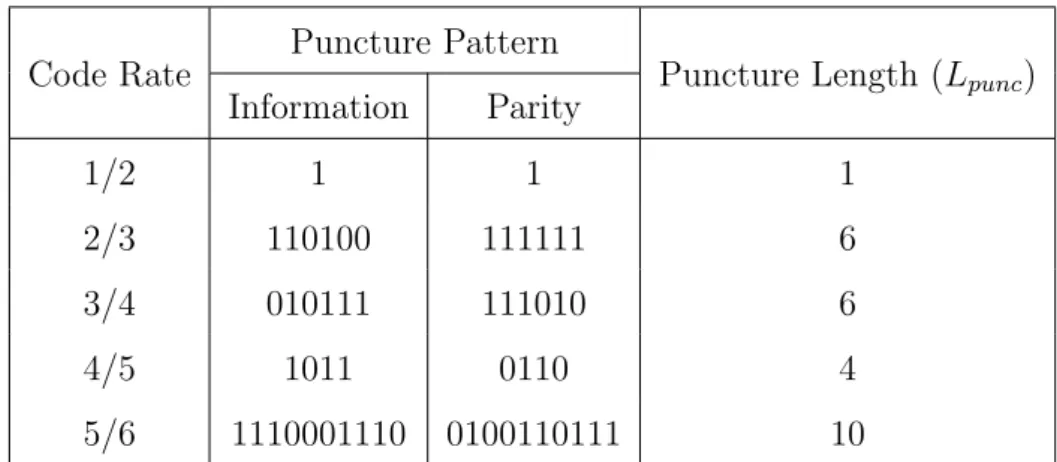
The equations in (3.4), which are constructed based on the parity check polynomials define the time-varying convolutional encoder, where u(D) and v(D) represent the infor-mation polynomial and parity polynomial respectively. Due to the time period is only 3, this property leads to significantly reduced hardware implementation complexity. Besides, the proposed LDPC convolutional code could support 5 code rates through puncturing. The puncturing patterns are shown in Table 3.1, the value 1 indicate that bit will be transmitted. In the other hand, the value 0 indicates that bit will be discarded every
Lpunc bits. Note that the LLRs of punctured bits are assumed to 0 at the receiver and
the decoding algorithm remains the same. Simulation results in [2] show that the BER performances are comparable to 16e Turbo decoder under AWGN channel for all code rates.
(D373+ D56+ 1)u(D) + (D406+ D218+ 1)v(D) = 0 (3.4a) (D457+ D197+ 1)u(D) + (D491+ D22+ 1)v(D) = 0 (3.4b) (D485+ D70+ 1)u(D) + (D236+ D181+ 1)v(D) = 0 (3.4c)
Table 3.1: Puncturing patterns for (491,3,6) LDPC convolutional code. Code Rate
Puncture Pattern
Puncture Length (Lpunc)
Information Parity 1/2 1 1 1 2/3 110100 111111 6 3/4 010111 111010 6 4/5 1011 0110 4 5/6 1110001110 0100110111 10
3.3
Encoding of LDPC Convolutional Codes
The encoding procedure of a rate R = b/c (b < c) LDPC convolutional code is described as follows. Let
u = (u0, u1, . . . , ut−1) (3.5)
be an information sequence, where ui = (u
(1)
i , u
(2)
i , . . . , u
(b)
i ). And assume that the coded
sequence after encoding is
v = (v0, v1, . . . , vt−1), (3.6) where vi = (v (1) i , v (2) i , . . . , v (c)
i ). The coded sequence v satisfies the constraint vHT = 0.
This equation could be further decomposed into equation (3.7) and directly used for encoding. Once all sub-matrices HT
0(t) have full rank, the encoder can be realized as a
shift-register based encoder. This property is called the fast encoding property, which guarantees that the constructed codes can be encoded continuously in real time [11].
vtHT0(t) + vt−1HT1(t) + . . . + vt−msHTms(t) = 0 (3.7)
Low-density parity-check convolutional codes are commonly expressed in terms of the polynomial representation. The transposed polynomial parity-check matrix HT(D) of the
convolutional code can be rewritten as
HT(D) = H0T + H1TD + H2TD2+ . . . + HMTDM. (3.8) We give an example of R = 3/8 time-invariant LDPC convolutional code with code
H(D) = 1 + D194 D158 D166 D144 0 D65 0 0 D97 D49 0 D203 D65 D37 1 0 0 D106 D83 D138 D48+ D132 1 0 0 0 0 1 0 0 0 D20 1 0 0 0 0 0 0 1 + D76 1 (3.9) Let vt = (v (0) t , v (1) t , v (2) t , v (3) t , v (4) t , v (5) t , v (6) t , v (7)
t ) be the coded bits and ut= (u
(0) t , u (1) t , u (2) t )
be the information bits. Given that v(1)t = u(0)t , vt(3) = u(1)t and vt(4) = u(2)t . The parity bits shown in (3.10) can be determined by solving (3.7).
vt(0) = vt(0)−194⊕ v(1)t−158⊕ vt(2)−166⊕ vt(3)−144⊕ v(5)t−65 (3.10a)
vt(2) = vt(6)−20⊕ vt(7) (3.10b)
vt(5) = vt(1)−106⊕ v(2)t−83⊕ vt(3)−138⊕ v(4)t−48⊕ vt(4)−132 (3.10c)
vt(6) = vt(0)−97⊕ vt(1)−49⊕ v(3)t−203⊕ vt(4)−65⊕ v(5)t−37 (3.10d)
vt(7) = vt(6)⊕ vt(6)−76 (3.10e) A systematic encoder can be obtained if we let the bottom (c− b) rows of the sub-matrices HT
0 (t) are identity matrix of size (c− b) × (c − b). For this special case, the
encoding equations can be simply summarized as follows.
v(j)t = u(j)t , j = 1, . . . , b, (3.11) vt(j) = b ∑ k=1 v(k)t h(j0−b,k)(t) + ms ∑ i=1 c ∑ k=1 vt(k)−ih(ji −b,k)(t), j = b + 1, . . . , c. (3.12) The encoding circuitry of an LDPC convolutional code is simple, analogous to the conventional convolutional code feedback encoder. The encoder can be implemented using multiplexers, XOR gates and c length (ms+ 1) shift-registers. If the constructed code is
time-invariant, the encoder connection is fixed. For the time-varying case which we are usually interested in, the encoder connections change periodically according to the check equations. It is worth to note that the encoding complexity of LDPC convolutional code is independent of the codeword length. Consequently, the encoder of LDPC convolutional
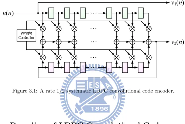
code enjoys the advantage of simple circuitry comparing to the traditional LDPC block code encoder. In addition, the ability to support arbitrary length of data frame provides more flexibility than LDPC block codes in many communication scenarios. The block diagram of a R = 1/2 systematic encoder for LDPC convolutional code is given in Figure. 3.1. The weight controller configures the encoder connections according to the parity-check polynomials. For low-cost implementation, the partial-syndrome former realization can be found in [13].
Figure 3.1: A rate 1/2 systematic LDPC convolutional code encoder.
3.4
Decoding of LDPC Convolutional Codes
The LDPC convolutional codes employ the same iterative message-passing algorithm as the decoding of LDPC block codes. Different from the LDPC block codes, the corre-sponding Tanner graph of an LDPC convolutional cods is infinite. Therefore, a pipeline decoder architecture is proposed as a finite sliding window to perform variable node and check node updates on the Tanner graph. Since the distance between two variable nodes that are connected to the same check node is at least (ms+ 1) time instants apart, the
decoding of two variable nodes can be performed independently. This concept allows the pipeline decoder to perform simultaneous decoding on different regions of the Tan-ner graph. The sliding window decoding on the TanTan-ner graph is implemented by using
processors corresponds to the number of iterative decoding iterations. Hence, the more processors are used, the more decoding performance increases. Studies have shown that LDPC convolutional codes could achieve the same near-Shannon-limit error performance as LDPC block codes. Recently, a comparison of LDPC block and LDPC convolutional codes indicates that, for the same decoding performance, the LDPC convolutional codes require less hardware costs than their corresponding block codes [14]. In addition, a detail investigation on several implementation issues such as stopping rules, decoding schedules, and several improvements to pipeline decoder architecture can be found in [15].
We give a R = 1/2 time-invariant (14, 3, 6) LDPC convolutional code in (3.13) as an example to illustrate the operation of the pipeline decoder on the Tanner graph. Figure. 3.2 shows the corresponding trellis diagram and the illustration of pipeline decoding. Since we add additional stage of register for pipelining, the length of sliding window in Figure. 3.2 is (ms+ 2) instead of (ms+ 1).
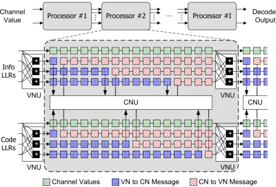
(1 + D5+ D11)u(D) + (1 + D7+ D14)v(D) = 0 (3.13) For a R = b/c (b < c) LDPC convolutional code decoder, it consists I identical processors operating in parallel, and each processor consists (J + 1)× c × (ms+ 1) first-in first-out
(FIFO) shift registers, (c− b) check node units and c variable node units. In particu-lar, this regular architecture insures low routing complexity comparing to the traditional LDPC block code. The decoding procedure is described in the following steps. Initially, all the shift registers in the pipeline decoder are filled with infinite ∞ because of the dummy zeros are the initial values in the encoder. As a new channel LLR is received, it is shifted in all the (J + 1) shift registers. Note that the LLR stored in the first shift register indicates the intrinsic value in the message-passing decoding. The next step is to operate the check node computations and then update the corresponding symbols which are con-nected to the same check node unit. Here we use the decoding algorithms such as belief propagation (BP) algorithm or normalized min-sum (NMS) algorithm in the bit-error-rate simulations. For the preceding (I − 1) processors, the variable node operations are performed just before the LLRs leave the processor. The last processor performs the hard decision for the information LLRs. Thus, the decoding procedure successively repeats the shifting step and appropriate node updates. As long as the initial decoding delay has elapsed, a total of I× (ms+ 1) time units, the pipeline decoder outputs a decoded data
stream continuously.
Chapter 4
Proposed Techniques for LDPC
Convolutional Codes
In previous chapter, we have introduced many important properties of LDPC convo-lutonal codes, including near Shannon limit performance, variable length of data frame, flexible code-rate through puncturing, simple encoding circuitry, and low routing com-plexity in the decoder architecture. However, LDPC convolutional codes rarely appear in system specification due to its bottlenecks of the long decoding latency, high power con-sumption, and low-to-moderate decoding throughput. The maximum measured through-put in previous literatures was only 600Mb/s and difficult to compete with LDPC block codes [16] [17].
In this thesis, we focus on the following three critical issues to design a high per-formance LDPC convlutional code decoder. Firstly, more processor numbers can obtain better decoding performance but extend longer latency with similar throughput. Sec-ondly, high node-level parallelism can achieve higher throughput but cause larger message bandwidth and severe memory conflict in memory-based FIFO architecture. Thirdly, a register-based FIFO architecture can support unlimited bandwidth but yield expensive power and area costs. To overcome these three issues, this thesis propose a new design approach which combines algorithm-level, node-level, bit-level optimization, and a hybrid-partitioned FIFO to achieve over 2Gb/s throughput with competitive power consumption and chip area.
4.1
Algorithm-Level Optimization
4.1.1
Flooding Scheduling
The message passing schedule is the order of propagating messages between check nodes and variable nodes over the Tanner graph. For decoding LDPC codes, the standard message-passing decoding schedule is the flooding schedule. According to the flooding schedule, the messages are passed in parallel between nodes. In each iteration, all the check nodes are updated simultaneously using the variable-to-check messages. Then, followed by updating all the variable nodes using the check-to-variable messages. Although the flooding scheduling is suited for parallel implementation, it is inefficient due to its low decoding convergence speed. Figure. 4.1 shows the conventional decoder architecture of (14, 3, 6) LDPC convolutional code given in (3.13). We can see that the variable nodes are performed until the messages are all transferred into the check-to-variable messages in the decoder.
We plot the floating point simulation results of (491, 3, 6) LDPC convolutional code with flooding schedule in the following figures. Figure. 4.2 depicts the BER performance under different decoding iterations at R = 1/2. We also compare the performance using different decoding algorithms such as log-BP algorithm, min-sum algorithm, and normal-ized min-sum algorithm. In Figure. 4.3, the dependence of the BER on the number of processors I at different SNRs using flooding schedule is shown. The results are simulated using the NMS algorithm with scaling factor 0.75. In Figure. 4.4, we present the BER performance under different code-rates through puncturing with 50 iterations. Compar-isons of log-BP algorithm and normalized min-sum algorithm with scaling factor 0.75 are also given.
Figure 4.1: Conventional decoder architecture. 1 1.5 2 2.5 3 3.5 10−5 10−4 10−3 10−2 10−1 100 Eb/No(db) BER Uncoded I = 10, Min−Sum
I = 10, NMS with scaling factor 0.75 I = 10, NMS with scaling factor 0.875 I = 30, Min−Sum,
I = 30, NMS with scaling factor 0.75 I = 30, NMS with scaling factor 0.875 I = 50, Min−Sum,
I = 50, NMS with scaling factor 0.75 I = 50, NMS with scaling factor 0.875 I = 50, Log−BP
0 20 40 60 80 100 120 140 160 10−5 10−4 10−3 10−2 10−1 Number of processors BER SNR = 1.2 SNR = 1.3 SNR = 1.4 SNR = 1.5
Figure 4.3: The dependence of the BER on the number of processors I at different SNRs.
1 2 3 4 5 6 10−5 10−4 10−3 10−2 10−1 100 Eb/No(db) BER R = 1/2, Log−BP R = 2/3, Log−BP R = 3/4, Log−BP R = 4/5, Log−BP R = 5/6, Log−BP R = 1/2, NMS R = 2/3, NMS R = 3/4, NMS R = 4/5, NMS R = 5/6, NMS
4.1.2
On-Demand Variable Node Activation (OVA) Scheduling
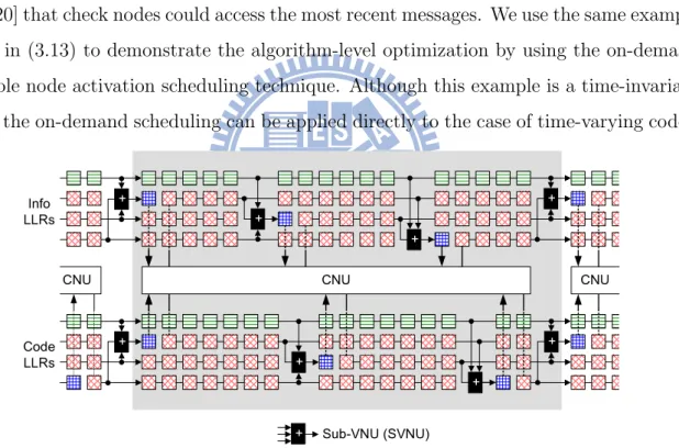
Studies have shown that the message-passing schedule affects the rate of decoding convergence and computational complexity. If we observe the standard decoding schedule, namely, the flooding scheduling, the variable node units are activated only once before the values leave the processor. Most messages are shifting while few messages are updating in a processor. Thus, this scheduling is inefficient without utilizing the recent updated information. For increasing the convergence speed, sequential scheduling are introduced in decoding LDPC block codes. Recently, an on-demand variable node activation schedule is proposed in [18] to accelerate the decoding convergence speed for LDPC convolutional code. The main idea is to change the variable node activation location leaving from the processor to the position right before each check node input. This on-demand variable node activation scheduling is very similar to the layered decoding in LDPC block codes [19] [20] that check nodes could access the most recent messages. We use the same example given in (3.13) to demonstrate the algorithm-level optimization by using the on-demand variable node activation scheduling technique. Although this example is a time-invariant code, the on-demand scheduling can be applied directly to the case of time-varying codes.
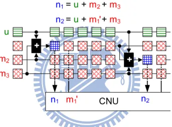
Figure 4.5: Processor architecture of on-demand variable node activation scheduling.
It can be seen from Figure. 4.5, a variable node unit (VNU) can be disassembled into
J sub-VNUs (SVNUs) and distributed within a processor. Before each check node unit is
activated, the sub-VNU calculates single variable-to-check message instead of calculating
be obtained by the partial computation of the variable nodes, and then these updated messages could be used to compute the remaining variable-to-check messages. The major difference from the standard decoding schedule is the order of updating procedures, and it is worth to note that the both computational complexity is the same.
To be more specific, in Figure. 4.6, n1 is a variable-to-check message which is obtained
by the summation of the intrinsic channel value u and two check-to-variable messages m2
and m3. Then this recently generated n1 is accessed by the check node unit immediately
to compute new check-to-variable message m′1. Also, the message m′1 is available for next sub-VNU to calculate a new variable-to-check message n2 for further check node updating
within the same iteration. It is clear that the frequency of message passing between check node and variable node is significantly increased. Using this scheduling, the messages can flow faster through the Tanner graph.
Figure 4.6: The illustration of on-demand variable node activation scheduling.
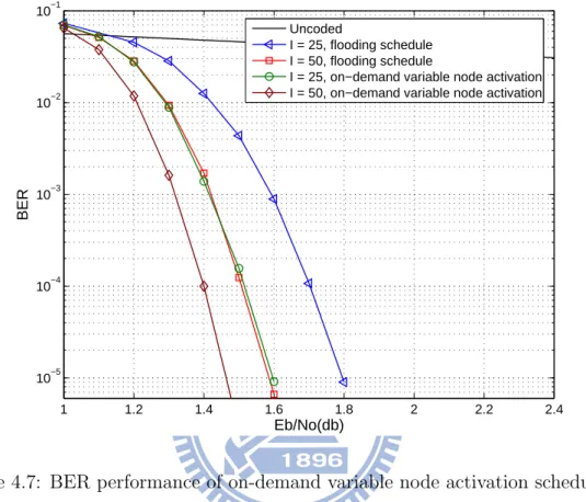
In Figure. 4.7, we show the floating point BER performance comparisons of stan-dard schedule versus on-demand schedule for a (491, 3, 6) time-varying LDPC convolu-tional code. It can be seen that the performance which uses on-demand schedule with 25 iterations is almost identical to the performance that uses standard schedule with 50 iterations. This indicates that the on-demand schedule converges twice faster than the standard schedule due to making use of the most recent information. In other words, the on-demand variable node activation scheduling allows the decoder to improve per-formance and achieve a lower BER for the same number of iterations. Therefore, for
and initial decoding delay are reduced nearly by half comparing to the standard schedul-ing. Figure. 4.8 shows that on-demand variable node activation schedule has a faster convergence speed than flooding schedule for all iterations. Figure. 4.9 gives the BER performance of NMS algorithm with scaling factor 0.75 using on-demand variable node activation schedule with the rates ranging from 1/2 to 5/6.
1 1.2 1.4 1.6 1.8 2 2.2 2.4 10−5 10−4 10−3 10−2 10−1 Eb/No(db) BER Uncoded I = 25, flooding schedule I = 50, flooding schedule
I = 25, on−demand variable node activation I = 50, on−demand variable node activation
0 20 40 60 80 100 120 140 160 10−5 10−4 10−3 10−2 10−1 Number of processors BER SNR = 1.2, flooding SNR = 1.3, flooding SNR = 1.4, flooding SNR = 1.5, flooding SNR = 1.2, OVA SNR = 1.3, OVA SNR = 1.4, OVA SNR = 1.5, OVA
Figure 4.8: The dependence of the BER on the number of processors I at different SNRs using on-demand variable node activation schedule.
1 2 3 4 5 6 7 10−5 10−4 10−3 10−2 10−1 100 Eb/No(db) BER R = 1/2, I = 50, flooding R = 2/3, I = 50, flooding R = 3/4, I = 50, flooding R = 4/5, I = 50, flooding R = 5/6, I = 50, flooding R = 1/2, I = 25, OVA R = 2/3, I = 25, OVA R = 3/4, I = 25, OVA R = 4/5, I = 25, OVA R = 5/6, I = 25, OVA R = 1/2, I = 50, OVA R = 2/3, I = 50, OVA R = 3/4, I = 50, OVA R = 4/5, I = 50, OVA R = 5/6, I = 50, OVA
4.1.3
OVA Scheduling with Concealing Channel Values
Since the equations in Figure. 4.6 of these two variable-to-check messages n1 and n2
have common terms u, we may calculate n2 from n1by deducting m2and adding m
′
1. Each
sub-VNU can be further disassembled into a pre-SVNU and a post-SVNU. The pre-SVNU performs the subtraction operation, and the post-SVNU performs the addition operation. Consequently, the channel values are concealed in variable-to-check messages. We named this newly proposed technique the on-demand variable node activation scheduling with concealing channel values. Figure. 4.10 illustrates the procedure to conceal the channel values and the corresponding pipeline decoder architecture is presented in Figure. 4.11.
Figure 4.10: The illustration of on-demand variable node activation scheduling with con-cealing channel values.
Figure 4.11: Processor architecture of on-demand variable node activation scheduling with concealing channel values.
The original processor architecture requires c × (J + 1) × (ms + 2) shift registers.
c× J × (ms+ 2). Assume that the quantization of messages is chosen as 6 bits and J
equals 3 in the decoder implementation. The storage requirement of original processor architecture is
6 bits× 8 rows × (ms+ 2) = 48× (ms+ 2) bits.
For example, in Figure. 4.11, the register in red requires 6 bits and the register in blue requires 8 bits. The storage requirement of our proposed processor architecture is
(6 bits× 4 rows + 8 bits × 2 rows) × (ms+ 2) = 40× (ms+ 2) bits.
Thus, the storage space of channel values can be removed from processors to save 17% memory. Although the channel values are concealed, the decoding results are identical to the scheduling without concealing channel values. Moreover, with our proposed concealing channel values technique, the storage requirements of the decoder are further reduced.
Figure. 4.12 shows the fixed point simulation of the (491, 3, 6) LDPC convolutional code with 5 iterations using normalized min-sum algorithm with scaling factor 0.75. We can see that the quantization (6, 2) for the LLRs, namely 4-bit for integer part and 2-bit for fraction part, has the minimum costs but with acceptable performance loss. Finally, we implemented 5 processors in our decoder chip. Figure. 4.13 is the BER performance of the rate-compatible (491, 3, 6) time-varying LDPC convolutional code under AWGN channel. In contrast to log-BP algorithm with 10 processors, the proposed algorithm with 5 processors can achieve similar or even better performance in all code-rates. There-fore, only half number of processors are required under the same performance, leading to half decoding latency reduction as well.
1 1.5 2 2.5 3 3.5 10−5 10−4 10−3 10−2 10−1 Eb/No(db) BER floating point fixed point (5, 2) fixed point (5, 3) fixed point (6, 2) fixed point (6, 3) fixed point (7, 3) fixed point (7, 4)
Figure 4.12: Fixed-point simulation results using OVA scheduling with 5 iterations.
Figure 4.13: BER performance of log-BP algorithm (floating-point) and our proposed scheduling in normalized min-sum algorithm with scaling factor 0.875 (fixed-point (6,2)) under AWGN channel.
4.2
Node-Level Optimization
4.2.1
Folding Architecture
In the original pipeline decoder architecture, a number of processors are concatenated together to decode on different regions over the Tanner graph simultaneously, thus the decoding is parallel in the iteration dimension. Assume the decoder can operate at fclk
MHz clock frequency, since the decoder can only decode one bit in one cycle, the infor-mation throughput will be limited to only fclk Mb/s. For high-speed applications, the
parallelization for LDPC convolutional code encoder and decoder is desirable. In the literatures, the concepts of node level parallelization are proposed in [21]. However, their decoder architecture requires the shuffle networks to overcome the problem of memory misalignments. Furthermore, the parallelism over a hundred is necessary to achieve the decoding throughput of 1 Gbps.
In order to provide a solution with lower complexity, we propose the folding technique for node level parallelization to design high throughput LDPC convolutional code encoder and decoder. The idea of folding technique is to look ahead the bits that are going to participate in the encoding or decoding operations. For parallel encoder using folding technique, total ρ information bits can be encode at the same time instant, where ρ is defined as the folding factor or the parallelization factor. The length of delay lines in the encoder are folded by a factor of ρ. And the XOR gate for encoding operation have to duplicate to ρ units. Although the similar parallel encoder architecture has been proposed in [22], the parallel encoder architecture they proposed requires large multiplexers for phase selection. For our folding technique, the parallelism is chosen as the multiple of time period. This allows the original time-varying encoding connections to transfer to fixed time-invariant connections. Thus, the multiplexers are no longer required in our encoder architecture, which is the major difference from [22].
Figure. 4.14 shows the parallel decoder architecture using folding technique. It can be seen that each FIFO delay line in the conventional processor is folded to ρ FIFO delay lines. In other words, each FIFO delay line is segmented by ρ factor to support required bandwidth. With this modified FIFO structure, sufficient input data could be provided
shift register of length 16 is replaced by 3 shift registers of length 6. Namely, the decoding delay is reduced from 16 clock cycles to 6 clock cycles for a unit processor. Also, both check node units and variable node units are duplicated to ρ units. Using this approach, the decoder throughput becomes (ρ×fclk) Mb/s. However, the maximum value of folding
factor is restricted by the code structure. Generally, the larger constraint length LDPC convolutional codes with careful code constructions would allow higher folding factor. To be mentioned that folding technique primarily duplicates the combinational logic while the sequential circuits are only slightly increased. It is evident that the folding technique not only increases the decoder throughput, but also reduces the decoding delay by a factor of ρ at the same time.
Figure 4.14: Folding technique (only information part in shown).
Based on the conventional decoder architecture, Table. 4.1 presents a comparison of storage requirements and decoding latency for a unit processor with different fold-ing factors. It can be seen easily that foldfold-ing technique not only directly duplicates the throughput, but also significantly reduces the decoding latency. Moreover, this technique only slightly increases the hardware costs. In particular, the overhead of the duplication of check node units and variable node units is minor comparing to the overall cost of a processor. We apply the folding technique to the time-varying (491, 3, 6) LDPC convolu-tional code with period of 3. Since the shortest distance of adjacent check node accessing positions is 70− 56 = 14, the maximum folding factor of this code is 12. Therefore, a 12 times decoding throughput increase while the decoding delay is reduced from 493 clock cycles to 43 clock cycles for single processor.
Table 4.1: Comparison of hardware cost and decoding latency with different folding factors based on the conventional decoder architecture.
Folding factor ρ 1 3 12
Required bits for storage 23664 23904 24768
Number of CNUs 1 3 12
Number of VNUs 1 3 12
Throughput fclk 3× fclk 12× fclk
Decoding latency for a unit processor (cycles) 493 166 43
In addition, the concepts of parallelization can be described mathematically. Figure. 4.15 shows the parity-check matrix of (14, 3, 6) LDPC convolutional code given in (3.13). Given that folding factor ρ = 3, every 3 rows in the parity-check matrix can be grouped to form a rate R = 3/6 LDPC convolutional code with syndrome former memory ms = 5.
Figure 4.15: Parity-check matrix of (14, 3, 6) LDPC convolutional code.
From the graph illustration in Figure. 4.15, we can see that the polynomial parity-check matrix becomes H(D) = 1 1 D2+ D4 D5 0 D3 0 D2 1 1 D2+ D4 D5 D + D3 D4 0 D2 1 1 . (4.1)
The same result can be derived from the parity check polynomials of the LDPC convo-lutional code. Using the parity check polynomial representation, the parity-check matrix can be described as
(D2+ D7+ D13)u0(D) + (D2 + D9+ D16)v0(D) = 0 (4.2a)
Let X = D3, we can rewrite these equations as
(D2 + X2· D + X4· D)u0(D) + (D2+ X3+ X5· D)v0(D) = 0 (4.3a)
(D + X2+ X4)u1(D) + (D + X2· D2+ X5)v1(D) = 0 (4.3b)
(1 + X· D2+ X3· D2)u2(D) + (1 + X2· D + X4· D2)v2(D) = 0. (4.3c)
Given in (4.4), the polynomial parity-check matrix is the same as (4.1) if X is replaced by D. H(X) = 1 1 X2+ X4 X5 0 X3 0 X2 1 1 X2+ X4 X5 X + X3 X4 0 X2 1 1 . (4.4) We apply this procedure on the time-varying (491, 3, 6) LDPC convolutional code with period of 3. Let folding factor ρ = 3, the corresponding parity-check polynomials are listed in (4.5).
(D2+ D58+ D375)u0(D) + (D2+ D220+ D408)v0(D) = 0 (4.5a)
(D + D198+ D458)u1(D) + (D + D23+ D492)v1(D) = 0 (4.5b)
(1 + D70+ D485)u2(D) + (1 + D181+ D236)v2(D) = 0 (4.5c)
With X = D3, we can rewrite the equations as
(D2 + X19· D + X125)u0(D) + (D2+ X73· D + X136)v0(D) = 0 (4.6a)
(D + X66+ X152· D2)u1(D) + (D + X7· D2+ X164)v1(D) = 0 (4.6b)
(1 + X23· D + X161· D2)u2(D) + (1 + X60· D + X78· D2)v2(D) = 0. (4.6c)
Finally, we can obtain a rate R = 3/6 time-invariant (164, 3, 6) LDPC convolutional code, whose polynomial check matrix is shown in (4.7). The columns of the parity-check matrix are rearranged to ensure systematic encoding. If the folding factor is chosen as a multiple of time period , the folding technique allows the original time-varying code to transform into a time-invariant code. Thus, the multiplexers for the configuration of time-varying connection are saved. Moreover, if the time-invariant code has quasi-cyclic symmetries, the encoder complexity of tail-biting LDPC convolutional codes may be reduced. We simulate the performance of a family of LDPC convolutional codes derived from (491,3,6) LDPC convolutional code with folding factors 3, 6, 9 and 12. The BER
performance of these codes is shown in Figure. 4.16. We can see that these codes perform very similarly even if the syndrome former memories vary greatly. Also given in (4.8) is the parity-check matrix of the R = 12/24 (41, 3, 6) LDPC convolutional code.
H(D) = 1 D19 D125 1 D73 D136 D152 1 D66 D7 1 D164 D161 D23 1 D78 D60 1 (4.7) H(D)= 1 0 0 0 D5 0 0 0 0 0 0 D32 1 0 D34 0 0 0 0 0 0 0 D19 0 D38 1 0 0 0 0 0 0 D17 0 0 0 0 1 D41 D2 0 0 0 0 0 0 0 0 0 0 1 0 D6 0 0 0 0 D41 0 0 0 D15 1 0 0 0 D20 0 0 0 0 0 0 0 D31 1 0 0 0 D5 0 0 0 0 0 D18 0 1 0 D34 0 0 0 0 0 0 0 0 0 D38 1 0 0 0 0 0 0 D17 0 0 0 0 1 D41 D2 0 0 0 0 0 D40 0 0 0 0 1 0 D6 0 0 0 0 0 0 0 0 D15 1 0 0 0 D20 0 0 0 0 0 0 0 D31 1 0 0 0 D5 0 0 0 0 0 D18 0 1 0 D34 0 0 0 0 0 D16 0 0 0 D38 1 0 0 0 0 0 0 0 0 0 0 0 1 D41 D2 0 0 0 0 0 D40 0 0 0 0 1 0 D6 0 D19 0 0 0 0 0 0 D15 1 0 0 0 0 D4 0 0 0 0 0 0 D31 1 0 0 0 0 0 0 0 0 0 D18 0 1 0 D34 0 0 0 0 0 D16 0 0 0 D38 1 0 D 0 0 0 0 0 0 0 0 0 1 D41 0 D5 0 0 0 0 D40 0 0 0 0 1 0 0 0 D19 0 0 0 0 0 0 D15 1 (4.8) 1 1.1 1.2 1.3 1.4 1.5 1.6 1.7 1.8 1.9 2 10−5 10−4 10−3 10−2 10−1 Eb/No(db) BER m = 491, b = 1, c = 2, time−varying m = 164, b = 3, c = 6, time−invariant m = 82, b = 6, c = 12, time−invariant m = 55, b = 9, c = 18, time−invariant m = 41, b = 12, c = 24, time−invariant
Figure 4.16: Performance of the (491, 3, 6) LDPC convolutional code and the associated LDPC convolutional codes with different folding factors.
4.3
Bit-Level Optimization
4.3.1
Retiming Technique
According to the previous mentioned on-demand variable node activation scheduling with concealing channel values, the channel values are concealed in the variable-to-check messages. When the channel values are concealed within the summation values, the bit-width of each message should be adjusted to avoid truncation error. In the situation of w-bit channel value, the summation of one channel value and two check-to-variable messages needs (w + 2)-bit. Since the operations of pre-SVNU and post-SVNU are independent, they can be re-timed such that the messages between them only need (w + 1)-bit. From the illustration in Figure. 4.17, we observed that, as long as the computation of sub-VNU is completed before the check node accesses the messages, the result is identical to the original operation. In order to achieve a maximum saving in hardware cost, we let the computation of post-SVNU to perform at the position just before check node accessing the messages.
Figure 4.17: Retiming of sub-VNUs.
Figure. 4.18 depicts the bit-level optimized processor architecture, the message output from the check node unit is w-bit. The message between the subtraction and addition needs (w + 1)-bit. And the message output from the post-SVNU which concealed channel values requires (w + 2)-bit. In particular, the critical path of the conventional processor is dominant by the check node unit due to large sorters are required. Although the on-demand variable node activation scheduling with concealing channel values can accelerate the decoding convergence speed, it induces one more adder delay and results to a longer
critical path. With the retiming technique for sub-VNUs, the critical path from check node unit to post-SVNU could be diminished by one adder delay. As a consequence, the retiming of sub-VNUs causes that the critical path of a unit processor remains the same while reducing memory requirements. This technique is especially useful to large constraint length LDPC convolutional codes for the long distance between two check node inputs.
Figure 4.18: Processor architecture with retimed sub-VNUs.
In Table. 4.2, we give a comparison of the storage requirements of three techniques which have been introduced so far. Assume that the quantization of LLRs is 6 bits, the required numbers of 6-bit, 7-bit and 8-bit registers for the (491, 3, 6) LDPC convolutional code with folding factor ρ = 12 are compared. When the OVA schedule with concealing channel values is adopted, the storage requirements is reduced by around 17%. With
Table 4.2: Comparison of the storage requirements with different techniques.
6-bit reg. 7-bit reg. 8-bit reg. Total required bits
Standard schedule 4128 0 0 24768
OVA scheduling with concealing channel values 2064 0 1032 20640
Retiming the sub-VNUs 2064 960 72 19680
4.4
Hybrid-Partitioned FIFO
There are two kinds of architectures for implementation of the LDPC convolutional code decoder in the literature, based and memory-based architecture. The register-based architecture enjoys the advantage of bandwidth flexibility, thus higher throughput can be easily achieved using folding technique. However, the large numbers of required registers would cause large hardware cost and high power consumption. The first ASIC realization using register-based decoder architecture is proposed in [23]. Although the memory-based architecture saves the power consumption and silicon area, the problem of memory access collisions is serious when high node parallelization is used. In the mean-time, folding technique could increase throughput, however it will divide the FIFOs into more pieces and make it difficult to use memory-based decoder architecture. In [24], the memory-base decoder architecture are used for FPGA implementations.
For time-varying LDPC convolutional codes with large folding factor, neither register-based FIFO nor memory-register-based FIFO is suitable. Therefore, we present a hybrid-partitioned FIFO structure to support large bandwidth requirement and also minimize the power con-sumption.
Figure 4.20: Processor architecture after merging sectors into memories.
Figure. 4.19 shows the illustration of the hybrid-partitioned FIFO structure. The first step of this technique is to calculate the length of the longest continuous sectors of every folded row. We only consider the continuous section of shift registers without messages accesses. Then the sectors are to be merged into one memory bank together, where the depth of the memory bank is the minimum value of the sector lengths. If the original sector is larger than the memory depth, the excess part is still stored in registers. This procedure continues to merge sectors until the memory depth is less than a pre-defined parameter. As shown in Figure. 4.20, the longest lengths of continuous sectors within the information part of the processor are 5, 4 and 4. Hence, the depth of the memory is 4 because of the minimum length of these 3 sectors is 4.
Note that this simple example is only for illustration. For the LDPC convolutional code with larger constraint length, the lengths of continuous sector within a processor will be longer. Large amounts of data are saved in the memory banks instead of registers, thus leads to a significant saving in power consumption. Besides, if large folding factor is employed, the number of continuous sectors in a processor will increase, and the lengths of continuous sectors will shorten. However, these continuous sectors can still be merged into several memory banks. This merge operation allows that the segmented and shorten
![Figure 1.1: Block diagram of channel coding procedure in the IEEE 802.16m transmit chain [1].](https://thumb-ap.123doks.com/thumbv2/9libinfo/8743556.204532/14.892.113.790.70.141/figure-block-diagram-channel-coding-procedure-ieee-transmit.webp)