針對數位訊號處理器中的巢狀迴圈考慮功率消耗的指令排程方法

全文

(1)國立交通大學資訊工程學系碩士論文. 針對數位訊號處理器中的巢狀迴圈考慮功率消耗的指令排程方法. Instruction Scheduling with Less Power Consumption for Nested Loop on DSP Architecture. 研究生：陳明志指導教授：陳正. 教授. 中華民國九十三年六月.

(2) 針對數位訊號處理器中的巢狀迴圈考慮功率消耗的指令排程方法. Instruction Scheduling with Less Power Consumption for Nested Loop on DSP Architecture 研究生：陳明志. Student: Ming-Chih Chen. 指導教授：陳正教授. Advisor: Prof. Cheng Chen. 國立交通大學資訊工程學系碩士論文. A Thesis Submitted to Institute of Computer Science and Information Engineering College of Electrical Engineering and Computer Science National Chiao Tung University in partial Fulfillment of the Requirements for the Degree of Master in Computer Science and Information Engineering June 2004 Hsinchu, Taiwan, Republic of China. 中華民國九十三年六月.

(3) 針對數位訊號處理器中的巢狀迴圈考慮功率消耗的指令排程方法研究生：陳明志. 指導教授：陳正教授. 國立交通大學資訊工程學系碩士班. 摘要隨著個人攜帶式應用產品的普及，對於影音資料與即時性資料的需求日益增加，因此，數位訊號處理器扮演的角色也日趨重要。如何能使資料即時且正確的展現在使用者面前成了一個重要的課題，而指令的排程在整個過程中是一個很關鍵的步驟。我們利用 Retiming 的觀念，設計了一個在有限資源情況下的排程方法，名為 Bottom Retiming Scheduling Method，改善了 Relax Push-Up Scheduling Method 會造成較大 maximum retiming depth 的缺點。另外，由於可攜帶式的產品大都由電池供電，如何降低消耗功率以延長使用時間，亦是一個重要的課題；我們以 Bottom Retiming Scheduling Method 為基礎，加入了 operand sharing 可以減少 switching activities 的觀念，設計了一個降低功率消耗的指令排程方法 Bottom Retiming with Operand Sharing Method。由實驗結果可以看出，這兩個方法都可以達到不錯的效果。. i.

(4) Instruction Scheduling with Less Power Consumption for Nested Loop on DSP Architecture Student: Ming-Chih Chen. Advisor: Prof. Cheng Chen. Institute of Computer Science and Information Engineering National Chiao Tung University. Abstract Because portable devices become popular, digital signal processing on images and real-time data are more and more important. How to process data correctly in real-time is one of the most interesting topics to be investigated. The instruction scheduling is an important step through the whole process. Under resources constraints, we use retiming technique to design a method named Bottom Retiming Scheduling Method. It overcomes the shortcoming of Relax Push-Up Scheduling Method which is a bigger maximum retiming depth. Besides data throughout, low power consumption is another important issue for portable devices. Based on Bottom Retiming Scheduling Method, we integrate the operand sharing technique which can reduce switching activities to design another method named Bottom Retiming with Operand Sharing Method for low power scheduling. The experimental results show the effectiveness of these methods.. ii.

(5) Acknowledgements I would like to express my sincere thanks to my advisor, Prof. Cheng Chen, for his supervision and advice. Without his guidance and encouragement, I could not finish this thesis. I also thank Prof. Jyj-Jiun Shann and Dr. Guan-Joe Lai for their valuable suggestions. There are many others whom I wish to thank. My thanks to Yi-Hsuan Lee for her kindly advice suggestion. Ming-Tien Chang, Chien-Wei Chen, Shun-Min Hsu, Wen-Pin Liu, Chia-Chun Lee and Wei-Fen Yang are delightful fellows, I felt happy and relaxed because of your presence. Finally, I am grateful to my dearest family. I also send my sincere thanks to my best friends, Shuo-Zhan Ho and Jing-Yuan Lin. They accompany me all the time.. iii.

(6) Table of Contents 摘要…………………………………………………………………………………..............…i Abstract…………………………………………………………………………….............…..ii Acknowledgements....................................................................................................................iii Table of Contents……………………………………………………………………...............iv List of Figures………………………………………………………………………................vi List of Tables.………………………………………………………………………..............viii Chapter 1. Introduction…………………………………………………………….............…..1 Chapter 2. Fundamental Background and Related Work…………………………................…3 2.1 Modeling the Problem......................................…………………………….............…3 2.2 Retiming an MDFG..……………………………………………………….................5 2.3 Related Work.................................................................................................................9 2.3.1 Push-Up Scheduling Method.............................................................................9 2.3.2 Relax Push-Up Scheduling Method.................................................................11 2.3.3 List Scheduling for Low Power.......................................................................12 Chapter 3. Bottom Retiming Scheduling Method……………….............................................13 3.1 Motivation……………………………………………………...................................13 3.2 Basic Concepts…………………………………………………................................14 3.3 Bottom Retiming Scheduling Algorithm.....…………………………….............…..17 3.4 Experimental Results..................................................................................................24 3.4.1 Evaluating the Execution Time........................................................................25 3.4.2 Performance Evaluation...................................................................................25 Chapter 4. Bottom Retiming with Operand Sharing Method………………………...............30 4.1 Motivation……………………………………………………...................................30 4.2 Grouping Nodes……………………………………………………..........................31 4.3 Bottom Retiming with Operand Sharing Algorithm...................................................38 4.4 Experimental Results..................................................................................................40 4.4.1 Evaluating Operand Reutilizations..................................................................40 4.4.2 Preliminary Performance Evaluations.............................................................41 Chapter 5. Conclusion and Future Work……………………………………………...............46 iv.

(7) 5.1 Conclusion…………………………………………………………………..............46 5.2 Future Work……………………………………………………………….............…47 Bibliography………………………………………………………………………..................48 Appendix A...............................................................................................................................52. v.

(8) List of Figures Figure 2.1. High-level language code of a DSP program………………..............…………4. Figure 2.2. An equivalent two-dimensional data flow graph.……………...……................4. Figure 2.3. Cell dependence graph………………….………………………….............…..5. Figure 2.4. The retimed MDFG by retiming function r…………………………................6. Figure 2.5. Retimed cell dependence graph…………………………………….............….7. Figure 2.6. An example of illegal retiming………………………………………...............9. Figure 3.1. Formula of ML…...………...……………..……………..…………................15. Figure 3.2. An partial schedule of an MDFG …..………………………………...............16. Figure 3.3. An MDFG modeling Floyd-Steimberg problem………………….............…..18. Figure 3.4. Scheduling information…………………………………………….............…18. Figure 3.5. The algorithm of Assign function…………………………………….............19. Figure 3.6. An example of the multidimensional delay counting function…….................21. Figure 3.7. Bottom Retiming Scheduling Algorithm……………………....…..................23. Figure 3.8. The retiming function………………………………………………...............23. Figure 3.9. The retimed MDFG and scheduling sequences of BRSM…………...............24. Figure 3.10. The execution time of benchmarks…………………………………...............28. Figure 4.1. An MDFG……………………..……………………………………...............32. Figure 4.2. The final schedule and an retimed MDFG…………………………................32. Figure 4.3. The algorithm of Group…………………….………………………...............34. Figure 4.4. Example for available continuous cycles……………………………..............34. Figure 4.5. The algorithm of Allocation……………...…………………………...............35. Figure 4.6. The algorithm of BROS……………………………………………................37. Figure 4.7. The information of scheduling nodes…………...………………….............…39. Figure 4.8. Scheduling sequences……………………..………………………….............39. Figure 4.9. The retimed MDFG and the retiming function.….…………………...............39. Figure 4.10. Operand reutilizations and execution time of Floyd-Steimberg……...............43. Figure 4.11. Operand reutilizations and execution time of 2-D Filter……………..............43. Figure 4.12. Operand reutilizations and execution time of IIR Section…………...............44 vi.

(9) Figure 4.13. Operand reutilizations and execution time of Transmission Line…................44. Figure 4.14. Operand reutilizations and execution time of DFT…………………..............45. vii.

(10) List of Tables Table 3.1 The available number of functional units of every benchmark………..…..............26 Table 3.2 The schedule vector and maximum retiming depth of every benchmark.................26 Table 4.1 The schedule vector and maximum retiming depth………………………..............41. viii.

(11) Chapter 1. Introduction In embedded system, high performance Digital Signal Processing（DSP）used in image processing, multimedia, wireless security, etc., needs to be processed not only with high data throughout but also with low power consumption [14]. These applications usually contain time-critical sections consisting of nested loops of instructions. The optimization of such loops, considering processing resource constraints, is required in order to improve their computational time [6]. Push-Up Scheduling Method (PUSM) [4] and Relax Push-Up Scheduling Method (RPUSM) [6] are retiming-based methods used to schedule instructions of nested loops under resources constraint. They can fully utilize functional units to achieve the minimum static schedule length, and RPUSM can further select a better schedule vector to reduce the entire execution time. However, they usually result in a bigger maximum retiming depth, which will longer prologue and epilogue and increase the entire execution time. Hence, in this thesis, we propose a method named Bottom Retiming Scheduling Method (BRSM) to overcome this shortcoming. In our BRSM, it can result in a smaller maximum retiming depth. From the experimental results, it shows that BRSM gives an improvement from 20.98% to 41.13% over the RPUSM in Floyd-Steimberg problem with various loop indexes [7]. As for low power scheduling, many techniques used for nested loops have been studied [2-6, 10-16, 19]. Based on operand sharing approach, a loop pipelining methodology to reduce both latency and power is first proposed in [13]. After that, a list-based loop pipelining technique is proposed to first minimize power and then maximize throughout [12]. Since list scheduling only considers the node with highest priority in ready list, it can’t get an optimal solution when the number of functional units is more than one in every scheduling step. In order to fully utilize functional units and reduce power consumption, we integrate the operand sharing technique into BRSM to design another method, Bottom Retiming with Operand -1-.

(12) Sharing method (BROS). It can bind operations with a common operand into the same functional unit and result in a smaller maximum retiming depth. BROS has advantages of BRSM and the operand sharing technique. From the experimental results, we can find that the performance of BROS is very close BRSM, and operand reutilizations are very high. This thesis is organized as follows. In chapter 2, we will introduce the fundamental background and the related work. In chapter 3, BRSM is presented in detail, and the experimental results are shown. BROS is finely presented in chapter 4, and the corresponding experimental results are shown. Finally, we conclude our thesis in chapter 5, and list the future work of our research.. -2-.

(13) Chapter 2. Fundamental Background & Related Work In this chapter, we will introduce the Multidimensional Data Flow Graph (MDFG) to model the nested loop to be scheduled. Then, the retiming technique will be presented. Finally, we will go through some related work, including Push-up Scheduling Method [4], Relax Push-up Scheduling Method [6], and List Scheduling for Low Power Method [2].. 2.1 Modeling the Problem [4-5] Multidimensional data flow graph (MDFG) is used to model the nested loop to be scheduled [4, 6, 24-26]. Definition 2.1 defines what an MDFG is.. Definition 2.1. A Multidimensional Data Flow Graph (MDFG) G = (V , E , d , t ) is a node-weighted and edge-weighted directed graph, where V is the set of computation nodes, E is the set of dependence edges, d is a function from E to Zn, representing the multidimensional delays between two nodes, where n is the number of dimensions, and t is the computation time of each node.. Fig. 2.1 shows the high-level language code of a DSP program. We use d (e) = (d .x, d . y ) to represent any delay edge e in a two-dimensional data flow graph. The equivalent two-dimensional data flow graph is shown in Fig. 2.2. In this thesis, we assume that execution time of any operation is one time unit. An iteration is equivalent to the execution of each node in V of an MDFG G exactly once, i.e., the execution of one instance of the loop body [4]. An iteration is associated with a static. schedule, that is repeatedly executed for the loop. Iterations are identified by a vector. -3-.

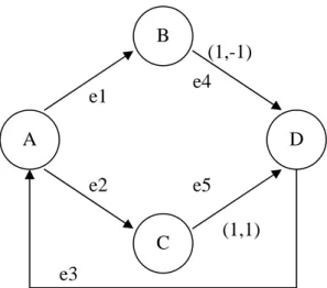
(14) B. for i = 1 to m for j = 1 to n { D:d(i,j)=b(i-1,j+1)*c(i-1,j-1); A: a(i,j)=d(i,j)*0.5; B: b(i,j)=a(i,j)+1; C: c(i,j)=a(i,j)+2; }. e1. (1,-1) e4. A. D e2. e5 C. (1,1). e3. Fig. 2.1 High-level language code of a DSP program. Fig. 2.2 An equivalent two-dimensional data flow graph. I, equivalent to a multidimensional index, starting from (1,1,...,1) . Inter-iteration dependencies. are represented by vector-weighted edges in an MDFG. For any iteration j, in an MDFG an edge from node u to node v with delay vector d (e) means that the computation of node v at iteration j depends on the execution of node u at iteration j − d (e) . An edge with delay (0,0,...,0) in an MDFG represents a data dependence within the same iteration. A legal MDFG must have no zero-delay cycle, i.e., the summation of the delay vectors along any cycle can’t be (0,0,...,0) .. Definition 2.2. A cell dependence graph (DG) of the MDFG G is the directed acyclic graph,. showing the dependences between copies of nodes representing an MDFG G.. The cell dependence graph is bounded by the dimensions of the problem which it represents [5]. A computational cell is the DG node that represents a copy of the MDFG, excluded the edges with delay vectors different from (0,0,...,0) . The computational cell is considered as an atomic execution unit. Fig. 2.3(a) shows the DG based on the replication of -4-.

(15) the MDFG in Fig. 2.1, and Fig. 2.3(b) shows its DG represented by computational cells.. 2.2 Retiming a Multidimensional Data Flow Graph [3-5] A multidimensional retiming r is a function from V to Zn that redistributes the nodes in the original dependence graph created by the replication of an MDFG G = (V , E , d , t ) [27]. A new MDFG Gr = (V , E , d r , t ) is created after applying retiming function r, and each iteration still has one execution of each node in G. The purpose of using retiming technique is to construct a new MDFG with better instruction level parallelism (ILP). The retiming vector r (u ) of a node u ∈ V represents the offset between the original iteration and the one after retiming. The delay vectors change accordingly to preserve dependencies. The retiming vector r (u ) of a node u represents delay components pushed into the edges u → v , and subtracted from the edges w → u , where u, v, w ∈ V . The execution of node u in iteration i which is represented by a multidimensional vector is moved to the iteration i − r (u ) . Here we give some definitions and properties of the retiming technique as follows.. -5-.

(16) Definition 2.3. For any MDFG G = (V , E , d , t ) , retiming function r, and retimed MDFG Gr = (V , E , d r , t ) , we define the retimed delay vector for every edge e in E, the retimed delay. vector for every path in G, and the retimed delay vector for every cycle in G, denoted as dr(e), dr(p), dr(l) respectively by the following formulas: e (a) d r (e) = d (e) + r (u ) − r (v) for every edge u ⎯ ⎯→ v , u, v ∈ V and e ∈ E ; p ⎯→ v , u, v ∈ V and p ∈ G ; (b) d r ( p ) = d ( p ) + r (u ) − r (v) for any path u ⎯. (c) d r (l ) = d (l ) for any cycle l ∈ G .. For example, Fig. 2.4 shows the retimed MDFG Gr after applying retiming function r on G. We can use the definition to obtain the retimed delay vector for every edge e in E. In Fig. 2.5(a), we show the retimed DG based on the replication of the MDFG in Fig. 2.4 and the retimed DG represented by computational cells is shown in Fig. 2.5(b). The retiming function applied to an MDFG may create prologue and epilogue. Prologue is the set of instructions that must be executed to provide the necessary data for the beginning of the iterative process. Epilogue is the set of instructions that must be executed to complete the process. These two sets of instructions are complementary. For example, in Fig. 2.5(a) the instruction D becomes the prologue, and the instruction A, B and C become epilogue for this problem. If the retiming function of node D of the MDFG in Fig. 2.2 is equal to (0,2) and the -6-.

(17) retiming function of other nodes is equal to (0,0), we can find that the instructions of the prologue and epilogue become more. So, the size of prologue and epilogue varies with the retiming function on the MDFGs. A schedule vector s is the normal vector for a set of parallel equitemporal hyperplanes that define the sequence of execution of the cell dependence graph. To get a schedule vector s, we can solve the inequalities d (e) ⋅ s ≥ 0 for every e ∈ E [5]. For example, (1,0) is a schedule vector of the MDFG in Fig. 2.2.. Definition 2.6. A legal MDFG G = (V , E , d , t ). that must have no zero-delay cycle is. realizable if there exits a schedule vector s for the cell dependence graph with respect to G, i.e., s ⋅ d ≥ 0 for any d ∈ G .. -7-.

(18) Definition 2.7. Given a realizable MDFG G, a legal multidimensional retiming for G is the. multidimensional retiming function r that transforms G into Gr, such that Gr is still realizable.. A legal multidimensional retiming on an MDFG G = (V , E , d , t ) requires that the execution sequence of the corresponding retimed DG does not contain any cycle. This constraint is enforced through the use of a schedule vector that supports the realization of the retimed graph. The selection of retiming function may result in illegal retiming. Fig. 2.6(a) shows an illegal retiming function applied to the MDFG in Fig. 2.2. By simple inspection of the cell dependence graph in Fig. 2.6(b), we can find that there exists a cycle created by the dependencies (0,1) and (0,-1). To get a legal multidimensional retiming r, we need to find a schedule vector s, such that s ⋅ d > 0 for any d ∈ G . For a two-dimensional problem, we choose s = ( s.x, s. y ) such that s.x + s. y is minimum. Then, a legal multidimensional retiming r of node u is any vector. orthogonal to s [5]. So, we can find that (0,1) is a legal retiming function on the MDFG in Fig. 2.2, and (1,0) is an illegal retiming function on the MDFG in Fig. 2.2. Further, we can have the corollary 2.1 [5].. Corollary 2.1. If r is a multidimensional retiming function orthogonal to a schedule vector s. that realizes an MDFG G = (V , E , d , t ) , and then (k × r ) is also a legal multidimensional retiming on that MDFG.. From the corollary 2.1, we know that the retiming function of every node in the retimed MDFG can be in the form (k × r ) . Here, r is called retiming base, and k is called retiming -8-.

(19) depth [6].. 2.3 Related Work [1-2, 4, 6] In this section, we’ll show how Push-Up Scheduling Method (PUSM) works, and then Relax Push-up Scheduling Method (RPUSM) will also be introduced. Finally, we will introduce the operand sharing technique and a scheduling method, List Scheduling for Low Power method (LPLS), using list scheduling method combined with operand sharing technique [2].. 2.3.1 Push-up Scheduling Method [4] In order to make the schedule length shorter, PUSM uses retiming technique to change the dependence in the MDFGs. PUSM will first analyze that if a node could be scheduled, and then use retiming technique to make the node schedulable as early as possible. Now, we define what a schedulable node as follows.. Definition 2.8. (Scheduling Conditions): Given an MDFG G = (V , E , d , t ) and a node u ∈ V ,. -9-.

(20) u is a schedulable node at a control step cs, if it satisfies one of the following conditions: (a) u has no incoming edges; (b) all incoming edges of u have a nonzero multidimensional delay; (c) all predecessors of u, connected to u by a zero-delay edge, have been scheduled to earlier control steps.. When scheduling an MDFG G by PUSM, it traverses G using BFS algorithm and checks that if the current traversing node satisfies the scheduling conditions or not. If the current traversing node satisfies the scheduling conditions, it will be scheduled in that control step. Otherwise, retiming technique will be used to make the node satisfy the scheduling conditions and be scheduled in that control step. During traversing G, every traversed node will record the multidimensional delay counting function MC (u ), u ∈ V . MC(u) represents the upper bound on the number of extra nonzero delays required by any path from roots of G to node u. Before traversing the MDFG G, a schedule vector s realizing G and a legal retiming r on G will be found. After traversing G, PUSM uses multidimensional delay counting function MC to calculate the retiming function of every node by the following formula: ∀u ∈ V , r (u ) = ( Max{MC (v), ∀v ∈ V } − MC (u )) × r PUSM can promise to get schedule with a minimum static schedule length. But PUSM ignores the effect of the schedule vector and the retiming depth. Both of them affect the execution time of a scheduled nested loop. Following, RPUSM provides a method to select a better schedule vector to reduce the execution time.. 2.3.2 Relax Push-up Scheduling Method [6] One of the main shortcomings of PUSM is that it doesn’t consider the effect of the schedule vector on the execution time. RPUSM finds that if the schedule vector could be kept as (1,0), the execution time is minimum as compared with other schedule vector different with - 10 -.

(21) (1,0). The author also proposed a method to check if (1,0) could be a schedule vector, as shown in theorem 2.1.. Theorem 2.1. For an MDFG G = (V , E , d , t ) , the retiming depth of any node u in V is rd(u).. We can use schedule vector s = (1,0) and retiming base r = (0,1) under one of the following two conditions which make the MDFG realizable: (a) If there doesn’t exist any delay vector (0, a ) for a > 0 in the original MDFG; (b). If there exists the delay vectors (0, a ) for a > 0 , and after finding out the retiming depth of every node in V we must make sure that rd (u ) + a > rd (v) for 0, a ) all u ⎯(⎯ ⎯→ v in the original MDFG;. Relax Push-up scheduling method (RPUSM) uses theorem 2.1 to modify PUSM to select a better schedule vector. The main difference is that RPUSM find the schedule vector and the retiming base after traversing an MDFG. Thus, RPUSM can use the multidimensional delay counting function MC obtained after traversing an MDFG to get the retiming depth of every node. RPUSM uses the retiming depth of every node to check if the conditions in theorem 2.1 are satisfied or not. If not, the same method of finding a schedule vector and a retiming base as PUSM will be performed. Although RPUSM provides a method to select (1,0) as a schedule vector, RPUSM, like PUSM, doesn’t consider the effect of the retiming depth of nodes. We’ll discuss this issue in chapter 3.. 2.3.3 List Scheduling for Low Power Method [2] There have been a few research results about power reduction using the operand sharing technique [1-2]. Here, we will briefly explain the operand sharing technique and then go - 11 -.

(22) through the key feature of list scheduling for low power method (LPLS). A functional unit in a data-path consumes both useful and useless power. It consumes useful power when it executes an operation and consumes useless power when there is an input operand transition while the functional unit is idle. The power consumption of a functional unit depends on the operand variability of its inputs. So, the operand sharing technique will try to bind operations with a common operand to the same functional unit such that the input activity of the shared functional unit decreases. In an MDFG, if a node has more than one outgoing edge, it reveals that the children of that node share the same data generated by that node. So, these children can be bind to the same functional unit in continuous cycles or non-continuous cycles without breaking by other operations. If two adjacent instructions executed on the same functional units have one common operand, it is called that one operand reutilization exists, or operand transition is reduced. One operand transition can reduce input activity of functional units. LPLS uses a list scheduling approach. The priorities of the operations of the ready-operation queue are set in such a way that operations sharing the same operand are scheduled in control steps as close as possible. So, the scheduling of the operations sharing the same operand is guided by giving more priority to the operations in the operand-ready queue. Because operations with common operands may be scheduled in non-continuous cycles without breaking by other operations, some nodes may be delayed. Thus, the schedule length becomes longer, and the utilization of functional units is decreased. Although LPLS can result in a schedule with well operand reutilization, the schedule length may be very long. In the chapter 3, we will present the bottom retiming scheduling method aiming at decreasing the retiming depth. In chapter 4, we will combine operand sharing technique with bottom retiming scheduling method to get a schedule with well operand reutilization and performance for reducing the power.. - 12 -.

(23) Chapter 3. Bottom Retiming Scheduling Method In this chapter, we will finely introduce Bottom Retiming Scheduling Method (BRSM). First, we will explain our motivation to propose a method reducing the execution time of a nested loop. Then, we will describe the main concept and principle of BRSM. Finally, we will give some basic experimental results. From the results, we can find that BRSM produces the schedule of a nested loop with less execution time compared with RPUSM.. 3.1 Motivation From the related work, we know that in order to schedule nodes as early as possible, PUSM first analyzes the scheduling conditions (definition 2.8). If necessary, it uses the retiming technique to make instructions satisfying the scheduling conditions to be schedulable earlier. Although PUSM can achieve minimum static schedule length, effects of the schedule vector and retiming depth did not be considered. Both of them affect the execution time of applications. In [6], the author proposed a method, RPUSM, to get a better schedule vector to reduce the execution time. Different from PRUSM, we focus on effects of the retiming depth. From Fig. 2.5, we find that some instructions become prologue and epilogue after retiming function is applied to an MDFG. Further, the prologue and epilogue will be longer while the retiming base is fixed and the maximum retiming depth, the maximum value of the retiming depth of all the nodes in a retimed MDFG, becomes bigger. That is to say, the optimized portion of the nested loop, the loop body, is decreased, and the un-optimized portion, prologue and epilogue, is increased. In order to reduce the execution time of nested loops, we have to increase the optimized portion of a nested loop. Thus, we need to decrease the maximum retiming depth. By observing RPUSM, we find that in order to make nodes schedulable as early as - 13 -.

(24) possible, many zero-delay edges will be changed to nonzero-delay edges. Thus, RPUSM will result in a static schedule with a bigger maximum retiming depth. In the following, we will introduce our BRSM to produce a static schedule with a smaller maximum retiming depth to reduce the execution time.. 3.2 Basic Concept In this section, basic concepts will be presented to explain how we decrease the maximum retiming depth under the minimum static schedule length with limited resources constraints. We describe how RPUSM works first. If m adders and n multipliers are available, RPUSM will schedule the first m add operations and the first n multiply operations in control step 1, the next m add operations and the next n multiply operations in control step 2,…until all operations are scheduled. If some node can’t be scheduled in that control step, RPUSM uses the retiming technique to change the delay dependences to make it schedulable earlier. Although RPUSM can fully utilize functional units to achieve minimum static schedule length, it will produce a static schedule with a bigger maximum retiming depth. A bigger maximum retiming depth will result in a longer prologue and epilogue to increase the execution time. We will propose a new method which not only fully utilizes functional units to achieve minimum static schedule length but also has a smaller maximum retiming depth. In order to fully utilize functional units, base on some information of architecture and applications, we can calculate the minimum static schedule length before scheduling. In a DSP application, it is usually composed of additions, multiplications, and assignments. Additions and multiplications are executed by adders and multipliers respectively. Assignments can be executed by adders or multipliers. To calculate the minimum static schedule length of some MDFG, denoted by ML(G), some information is needed, the total number. of. adders(A),. multipliers(M),. additions(ADD), - 14 -. multiplications(MUL),. and.

(25) assignments(AS). It costs ADD/A and MUL/M cycles to execute all additions and multiplications respectively. If no assignments exist, the bigger one of ADD/A and MUL/M is ML(G). If assignments exist, we need to calculate that how many cycles it costs to execute them. The formula for calculating ML(G) is shown in line 1 and line 2 of Fig. 3.1. Because assignments can be executed by adders or multipliers, we can calculate the maximum number of assignments executed by adders and multipliers, as shown in line 3 and line 4 of Fig. 3.1. Generally speaking, in order to get a schedule with a smaller maximum retiming depth, we need to reduce the number of edges requiring additional multidimensional delays after scheduling. In other words, if there are fewer edges changing delay dependences of the MDFG after retiming, there are fewer edges requiring additional multidimensional delays after scheduling. Thus, we know we need to make fewer edges changing delay dependences. In order to reduce such edges, we retain the delay dependences to schedule as many nodes as possible. And in order to fully utilize functional units, nodes have to be scheduled before. - 15 -.

(26) minimum static schedule length. Under minimum static schedule length and resources constraints, when a node u is schedulable in control step cs, there are three conditions as follows: (1) cs is smaller than minimum static schedule length, and there is an available functional units between control step cs and minimum static schedule length; (2) cs is smaller than minimum static schedule length, and no functional units is available between control step cs and minimum static schedule length; (3) cs is bigger than minimum static schedule length. We give an example to explain these three conditions. In Fig. 3.2(a), we assume that one adder and multiplier are available. The minimum static schedule is two. In control step 1, node A1 is schedulable and one adder is available in that control step which is satisfying condition 1. We schedule A1 in control step 1, as shown in Fig. 3.2(b). Then, node M1 and M2 are schedulable in control step 2 and one multiplier is available. Assume that M1 are scheduled first, as shown in Fig. 3.2(c). We can find that M2 is schedulable in control step 2 but no available functional units in that control step which is satisfying condition 2. Node A2 is schedulable in control step 3 and the minimum static schedule length equals to 2 which is satisfying condition 3. From these three conditions and under minimum static schedule length constraints, we can know which conditions will result in additional multidimensional delays. - 16 -.

(27) In condition 1, node u can be scheduled in some control step from cs to minimum static schedule length to retain the delay dependence. In other conditions, all incoming edges of node u require additional multidimensional delays to make u schedulable earlier. Based on above concepts, we will introduce Bottom Retiming Scheduling Algorithm in the next section.. 3.3 Bottom Retiming Scheduling Algorithm In this section, we will finely explain BRSM. Based on the above three conditions, we can use two functions, ES(u) and Assign(u), to decide when a multidimensional delay is needed. Given an MDFG G = (V , E , d , t ) and a node u ∈ V , the earliest starting time for the execution of node u, ES(u), is the first control step following the end of the execution of all predecessors of u by a zero-delay edge. It can be represented as: ES (u ) = Max{1, ES (vi } + t (vi )} for all vi preceding u by an edge ei such that d (ei ) = (0,0,...,0) . From the definition of ES(u), we can know ES(u) is the earliest time that node u can start to be scheduled. For example, in Fig. 3.3, ES(M1) = ES(M2) = 1, and ES(A1) = 2. Thus, ES(A2) = 3. In the following, we will introduce the function Assign(u) to record which control step node u assign to. Under minimum static schedule length and resources constraints, we would like to schedule node u in some control step to make incoming edges of u retaining their delay dependences. If that control step is smaller than minimum static schedule length and a functional unit is available in that control step, u will be scheduled in that control step. Thus, Assign(u) will equal to that control step. Or incoming edges of u will require additional multidimensional delays to make u schedulable earlier. Thus, Assign(u) will equal to an earlier control step in which a functional unit is available. Assign(u) can be determined as follows: (a) When node u is schedulable and one functional unit is available between control step, - 17 -.

(28) ES(u) and minimum static schedule length, Assign(u) equals to Min { cs , such that ES (u ) ≤ cs ≤ minimum static schedule length, and a functional unit is available in cs}; (b) When node u is schedulable and no function unit is available between control step ES(u) and minimum static schedule length, Assign(u) equals to Min{ cs, such that 1 ≤ cs ≤ ES (u ) − 1 , and a functional unit is available in cs}; (c) When node u is schedulable and ES(u) is bigger than minimum static schedule length, Assign(u) equals to Min{ cs, such that 1 ≤ cs ≤ ES (u ) − 1 , and a functional unit is available in cs}. From those, we know that if possible, Assign(u) will record an control step which can retain - 18 -.

(29) the delay dependences for node u, or Assign(u) will record an earlier control step to make u schedulable earlier. The algorithm of Assign is shown in Fig. 3.5. According to the definitions of ES(u) and Assign(u), we can determine when a multidimensional delay is needed by the following. If ES (u ) > Assign(u ) for node u, all incoming edges of u require additional multidimensional delays, because u is assigned to the control step earlier than ES(u). Inspecting from the function Assign, we find that the second and third condition result in. - 19 -.

(30) some edges requiring multidimensional delays. In order to avoid the second condition, more resources are required. In order to avoid the third condition, we have to avoid the earliest starting time of nodes being delayed. For example, in Fig. 3.3, node M1, M2, and M3 are schedulable in control step 1, and are scheduled in control step 3, 2, and 1 respectively. Thus, ES(A3) = 6. If M1, M2, and M3 are scheduled in control step 1, 2, and 3 respectively, ES(A3) = 4. In order to avoid ES(u) being delayed, we need to schedule nodes on critical path, the longest path, earlier. We will give every node a priority, and nodes on critical path are given higher priorities to be scheduled earlier. A BFS-like algorithm is used to assign priorities. The traversal direction is from leaves to roots. We can find that if the height of leaves is zero and the height of roots is highest, the nodes on longer path are at higher height. Thus, we prioritize nodes by their height. Priorities of all leaves equals to zero, and the priority of node u, P(u), is assigned by the following formula: P (u ) = Max{P(u ), P(vi ) + 1} for all vi succeeding u by an edge ei such that d (ei ) = (0,0,...,0) . For example, after prioritizing nodes in Fig. 3.3, priorities are shown in Fig. 3.4. We use two functions, ES(u) and Assign(u), to find which edges need for additional multidimensional delays. From the information, the retiming depth of every node can be found. The multidimensional delay counting function MC(u) is the upper bound on the number of extra nonzero delays required by any path from roots of G to node u. We can use it to compute the retiming depth of every node. If w precedes u by an edge requiring a multidimensional delay MC(u) = Max{MC(u),MC(w)+1}. Otherwise, MC(u) = Max{MC(u), MC(w)}. Fig. 3.6 is an example of computing the multidimensional delay counting function. Assume that edges A → B , D → E , C → F , and G → H require multidimensional delays. After the function MC(u) is calculated, the retiming depth of every node u equals to MC max − MC (u ) , where MCmax is the maximum retiming depth of the retimed MDFG. - 20 -.

(31) We use similar method proposed in [6] which uses the retiming depth of every nodes to check if (1,0) can be the schedule vector. It is shown in line 24 to line 33 of Fig. 3.6. From 0,a ) these lines, we know that if the condition ∀u ⎯(⎯ ⎯→ v, rd (u ) + a > rd (v) is satisfied, (1,0). can be the schedule vector. For BRSM and RPUSM, rd(u) equals to the maximum retiming depth. BRSM usually results in a smaller maximum retiming depth, so it has more chances to satisfy the condition and then select (1,0) as the schedule vector. The algorithm of BRSM is shown in Fig. 3.7. Now, we give an example of the MDFG in Fig. 3.3 to show how BRSM works. We assume that three adders and a multiplier are available. The priority of every node is shown in Fig. 3.4, and the minimum static schedule length equals to five. We start to schedule nodes. In control step 1, M1, M2 and M3 are schedulable nodes and scheduled in control step 1, 2, and 3 respectively, as shown in Fig. 3.9(b). In control step 2, A1 is schedulable. Although there is an available adder in control step 1, we don’t schedule A1 in that control step. Because we want to retain the delay dependences to schedule as many nodes as possible, A1 is scheduled in control step 2, as shown in Fig. 3.9(c). Then, A2, A3, and M4 are schedulable in control step 3, 4, and 5 respectively and scheduled in those control steps. A4 is schedulable in control step 6, but ML(G), equals to five. We need to make edge M 4 → A4 having a multidimensional delay to schedule A4 earlier. Since edge M 4 → A4 has a multidimensional delay, A4 can be - 21 -.

(32) - 22 -.

(33) scheduled in control step 1 and then A5 is schedulable in control step 2. The final schedule is shown in Fig. 3.9(d). From the final schedule we know that besides edge M 4 → A4 , edges A6 → A13 and A9 → A13 also need a multidimensional delay. The multidimensional delay counting function is shown in Fig. 3.4. Then, we find the schedule vector (2,1), and the retiming base (1,-2). Finally, the retiming depth and the retiming function are calculated, as shown in Fig. 3.4 and Fig. 3.8 respectively. The retimed MDFG is in Fig. 3.9(a). The maximum retiming depth equals to two. If this MDFG is scheduled by RPUSM or PUSM, the - 23 -.

(34) maximum retiming depth equals to six. In the next section, we use eight benchmarks to compare the performance of BROS and RPUSM.. 3.4 Experimental Results In this section, we will show some performance evaluations of the DSP benchmark. At first, we will introduce the formula of evaluating the execution time for nested loops and then compare the performance of RPUSH and BRSM. At the end, we will give an analysis of the comparison and conclude the advantage of BRSM.. - 24 -.

(35) 3.4.1 Evaluating the Execution Time In DSP applications, most nested loops are 2-dimensional loops. Thus, we use eight benchmarks to evaluate the performance of BRSM and they are all 2-dimensional DFG. In the following, we introduce the formula to execute the execution time of 2-dimensional loops whose indexes are m and n. Before applying the retiming technique to a 2-dimensional loop, its execution time can be represented by m × n × D , where D is the static schedule length. After applying the retiming technique, the execution time of a 2-dimensional loop can be divided into three parts, the loop body, the prologue and epilogue inside the first level loop, and the prologue and epilogue out of the nested loop. The formula of evaluating execution time of a 2-dimensional loop is shown as follows [6]: A(m − s 2 × d )(n − s1 × d ) + ( B + C )( s1 × m + s 2 × n − s1 × s 2 − 2 × d × s1 × s 2 ) + D × s1 × s 2 × d (d + 1). ------ (1) , where (s1,s2) is the schedule vector, d is the maximum retiming depth, A is the static schedule length after applying some algorithm for optimization, D is the static schedule length of an iteration after applying “List Scheduling”, B is the length of prologue inside the first level loop, and C is the length of epilogue inside the first level loop. Following, we use the formula to compare the performance of BRSM and RPUSM.. 3.4.2 Performance Evaluation Here, we have used eight benchmarks, shown in Appendix A, to evaluate the effect between BRSM and RPUSM. Loop indexes vary from 10 to 50 with various combinations for each benchmark. The available number of functional units for each benchmark is shown in Table 3.1. The principle of determining the number of functional units is to balance the execution time of total additions and multiplications in an iteration. After scheduled by BRSM - 25 -.

(36) FloydSteimberg. IIR Section. Transmission Line. IIR Filter. DFT. 2-D Filter. Forward Substitution. THC Solver. Adder. 3. 2. 2. 2. 2. 2. 1. 1. Multiplier. 1. 2. 1. 2. 1. 2. 1. 1. RPUSM. BRSM. Floyd Steimberg. IIR Section. Transmission Line. IIR Filter. DFT. 2-D Filter. Forward Substitution. THC Solver. Schedule vector. (2,1). (1,1). (1,0). (1,1). (1,1). (1,1). (1,1). (0,1). Maximum retiming depth. 6. 2. 2. 2. 2. 3. 2. 1. Static schedule length. 5. 4. 4. 4. 3. 9. 3. 2. Schedule vector. (2,1). (1,1). (1,0). (1,1). (1,1). (1,0). (1,0). (0,1). Maximum retiming depth. 2. 1. 2. 1. 1. 0. 1. 1. Static schedule length. 5. 4. 4. 4. 3. 9. 3. 2. and RPUSM, the schedule vector and maximum retiming depth are shown in Table 3.2. The execution time of each benchmark is shown in Fig. 3.10. From the Table 3.2, we find that after Floyd-Steimberg is scheduled by BRSM and RPUSM, they select the same schedule vector, but BRSM results in a smaller maximum retiming depth. Thus, the execution time of Floyd-Steimberg scheduled by BRSM is smaller than that scheduled by RPUSM, as shown in Fig. 3.10(a), and some other benchmarks have the similar results. When the number of iterations of Floyd-Steimberg equals to 10 × 10 , RPUSM can’t apply to this benchmark, because RPUSM results in the maximum retiming depth equal to six and schedule vector equal to (2,1). Thus, the minimal index of the first level loop is 12. For 2-D Filter [8], after scheduled by BRSM and RPUSM, BRSM selects (1, 0) as the schedule vector but RPUSM can’t. And BRSM results in a smaller maximum retiming depth. Thus, the execution time of 2-D Filter scheduled by BRSM is smaller than that scheduled by RPUSM , as shown in Fig. 3.10 (f) , and this circumstance also happens to the benchmark, Forward-Substitution [9], as shown in Fig. 3.10(g). After Transmission Line [4] is - 26 -.

(37) - 27 -.

(38) - 28 -.

(39) scheduled by BRSM and RPUSM, they result in the same schedule vector and maximum retiming depth. From Fig.3.10(c), we find that the execution time of Transmission Line scheduled by RPUSM is smaller than that scheduled by BRSM. This is because that the schedule length of prologue and epilogue inside the first level loop scheduled by RPUSM is smaller than that scheduled by BRSM. The benchmark, THC Solver [4], is just the opposite. From Fig. 3.10, if we inspect carefully, we find that the difference of the execution time of each benchmark is getting bigger while the number of iterations increases. This is because the prologue and epilogue inside the first level loop increase along with the number of iterations. This phenomenon can be observed by the formula (1). In 2-Dimensional Filter, BRSM can achieve the minimum schedule length without using the retiming technique. This is because that BRSM gives nodes on the longest path higher priority. Thus, these nodes can be scheduled as early as possible. As mentioned earlier, BRSM has more chances to select (1,0) as a schedule vector. 2-D Filter and Forward Substitution are two instances. From the evaluation results listed above, we find that BRSM is better than RPUSM. BRSM can result in a schedule with the smaller maximum retiming depth and have more chances to select (1,0) as the schedule vector. The smaller maximum retiming depth and (1,0) as the schedule vector can reduce the execution time of a nested loop. Thus, the execution time of a nested loop scheduled by BRSM is usually less than that scheduled by RPUSM. Next chapter, we’ll integrate operand sharing technique into BRSM for low power scheduling.. - 29 -.

(40) Chapter 4. Bottom Retiming with Operand Sharing Method In this chapter, we will introduce our second method named Bottom Retiming with Operand Sharing method (BROS). First, we’ll show how to group nodes with common operands. Then, BROS will be finely explained. Finally, some basic experimental results will also be shown.. 4.1 Motivation Low power becomes the critical design issue due to wide use of the portable devices, especially those powered by batteries [14]. Reducing switching activities is one of most important power optimization methods when the hardware is built up. Based on the energy model proposed by [14], the energy ES for a schedule S can be computed by L. L. k =1. k =1. (k ) E S = ∑ Pcycle = L × Pbase + ∑. ∑. Insti( k ). L. PInst ( k ) + ∑ i. k =1. ∑ SP. (k ). (i, j ). Insti( k ). where Pcycle is the power consumption of one control step in which several instructions can be executed, Pbase is the base power needed to execute one control step, PInsti is the basic power to execute an instruction Insti on a functional unit, SP(i,j) is the switching power caused by switching activities between Insti (current sub-instruction) and Instj (last sub-instruction) L. executed on the same functional unit, and L is the schedule length of S.. ∑∑. k =1 Insti( k ). PInst ( k ) is the i. summation of basic power consumptions for all instructions of an application. It doesn’t L. change with different schedules. L and. ∑ ∑ SP. (k ). (i, j ) will change with different. k =1 Insti( k ). schedules length. Therefore, in order to minimize the energy consumption of an application,. - 30 -.

(41) schedule length of applications and switching activities between instructions both need to be considered in scheduling. In the following, we will show how we consider both issues in scheduling.. 4.2 Grouping Nodes BRSM can produce a schedule with a smaller maximum retiming depth and smaller execution time of nested loops. And the operand sharing technique can reduce the input activities of functional units. Thus, in order to reduce the schedule length and switching activities, we intend to integrate the operand sharing technique into BRSM. Operand sharing technique tries to bind operations with a common operand to the same functional unit such that the input activity of the shared functional unit decreases. In the MDFG of Fig. 3.4, A6, A7, A8 and A9 share the same operand produced by A5. When we bind these four nodes in continuous cycles, three operand transitions in an iteration can be reduced. That is to say, there are three operand reutilizations in an iteration. In order to have as many as possible operand reutilizations in an iteration, we must make sure that operations with a common operand are scheduled in continuous cycles. Thus, we have to find out those operations first. We can use BFS-like method to traverse MDFGs. If the number of outgoing edges of the current traversing node is bigger than one, there is more than one operation sharing a common operand. Thus, by checking the number of outgoing edges of the current traversing node, we can determine if its children have to be grouped in an operand sharing set (SS).. In some cases, we group node u into some SS, but after scheduling, node u has different operands from other nodes in the same SS. For example, in Fig. 4.1(a), we assume that two adders are available, and the minimum static schedule length equals to two. From that MDFG we know A2 and A3 share the same operand produced by A1. In order to bind A2 and A3 in - 31 -.

(42) t he same functional unit, one of the possible schedules is shown in Fig. 4.2(a) and the retimed MDFG is shown in Fig. 4.2(b). Even though A2 and A3 are bound in the same functional unit and in continuous control steps, A2 and A3 share different operands, and no operand transition is reduced. We call such node, A2, as an unnecessary node of the SS. We can define an unnecessary node more formally as follows. If node u and v belong to the same SS sharing the data produced by w and a zero-delay path exists from some child of node v to u, u is an unnecessary node of the SS and will be deleted from the SS. Why a node is unnecessary is that in order to bind u and v in continuous cycles, we need to schedule u before schedule those nodes on the path from v to u. Some edges on that path usually require multidimensional delays to make u being scheduled earlier. The side effect is that edge w → u has a multidimensional delay but edge w → v doesn’t. The algorithm in Fig. 4.3 is used to find all the SSs of an MDFG and delete unnecessary nodes from SSs. For example, in Fig. 3.4, after we traverse the MDFG, we group A6, A7, A8 and A9 in one SS, and group A10, A11, A12 and A13 in another SS.. After finding out all the SSs of an MDFG, we’ll pre-schedule all the SSs in order to make sure that nodes in an SS are bound in the same functional unit in continuous cycles. Because one big SS will have more operand reutilizations than several small SSs, the SS with bigger - 32 -.

(43) - 33 -.

(44) size will be scheduled first. For example, one SS with eight elements has seven possible operand reutilizations, but two SSs with four elements have six possible operand reutilizations. Before we schedule an SS in continuous cycles, we have to check if any one functional unit is available in any |SS| continuous cycles, where |SS| means the size of an SS. The available continuous cycles is the maximum number of continuous cycles in which a functional unit is. available. For example, in Fig. 4.4, two adders are available and two nodes have been scheduled and the minimum static schedule length is four. The available continuous cycles of the two adders are two and three respectively. The maximum continuous cycles is the maximum number of the available continuous cycles of every functional unit of the same kind. For example, in Fig. 4.4 the maximum continuous cycles of adders is three. BRSM is under - 34 -.

(45) the minimum static schedule length with limited resources constraint, thus the maximum value of the maximum continuous cycles equals to the minimum static schedule length. If |SS| is bigger than the maximum continuous cycles, we have to subtract a subset with its size equal to the maximum continuous cycles from the SS, and this subset is pre-scheduled immediately. The remainder becomes a new SS. The algorithm in Fig. 4.5 is shown how to pre-schedule the SSs. For example, in Fig. 3.4, after applying the function Group, two SSs are found, {A6, A7, A8, A9} and {A10, A11, A12, A13}. After we pre-schedule these two SSs, the result is shown. in Fig. 4.8(a). In some cases, after applying BRSM to MDFGs, the maximum operand reutilizations would be decreased. For example, there are at most nine operand reutilizations in an iteration in Fig. 3.4. Three operand reutilizations are due to A6, A7, A8 and A9 sharing the data - 35 -.

(46) - 36 -.

(47) produced by A5. And six operand reutilizations are due to A10, A11, A12 and A13 sharing the data produced by A6 and A9. After applying BRSM to that MDFG, from the retimed MDFG in Fig. 3.9(a) we find that the maximum operand reutilizations in an iteration are seven. It is because that both operands of A13 are different from operands of A10, A11, and A12. In order to have as many as possible operand reutilizations in an iteration, we have to make sure that not only operations with a common operand are scheduled in continuous clock cycles, but also the maximum operand reutilizations in an iteration aren’t decreased. By using the two functions Group and Allocation, we can achieve the former one. In order to achieve the later one, we only need to make sure that for every node v such that v belongs to some SS and shares the data produced by node w, edge w → v has the same multidimensional delay. Thus, if some such edge requires an additional multidimensional delay, we make all the other edges having the same multidimensional delays. We call this behavior as adjusting. By adjusting, we can make sure that the maximum operand reutilizations in an iteration aren’t decreased. In the following, we’ll introduce BROS.. - 37 -.

(48) 4.3 Bottom Retiming with Operand Sharing Algorithm In order to integrate the operand sharing technique into BRSM, we have to modify the function Assign, used in BRSM. Assign(u) records the control step in which node u is scheduled. If node u belongs to some SS, u must have been scheduled. Thus, Assign(u) equals to the control step which u is scheduled in. If node u doesn’t belong to any SS, the data of Assign(u) is determined by the original definition as in chapter 3.. The algorithm shown in Fig. 4.6 is Bottom Retiming with Operand Sharing method (BROS). The adjusting behavior is from line 17 to line 19 in the algorithm. We give an example in Fig. 3.4 to show how BROS works. Assume that three adders and a multiplier are available. After prioritizing nodes, the priority of every node is shown in Fig. 4.7. The minimum static schedule length equals to five. Then, we find out two operand sharing sets,{A6, A7, A8, A9} and {A10, A11, A12, A13}, and then these sets are pre-scheduled, as shown in Fig. 4.8(a). The final schedule is shown in Fig. 4.8(b). Before applying the adjusting behavior, edges requiring multidimensional delays are M 4 → A4 , A5 → A6 , A5 → A7 , A5 → A8 , A5 → A9 , A6 → A10 , A6 → A11 , A9 → A10 and A9 → A11 . The data sharing by. A10 and A11 is different from the data sharing by A12 and A13. But when the adjusting. behavior is applied, A10, A11, A12, and A13 share the same data produced by A6 and A9. The multidimensional delay counting function and the retiming depth of every node are shown in Fig. 4.7. The schedule vector (2,1) and the retiming base (1,-2) are calculated. Finally, the retiming function and the retimed MDFG is shown in Fig. 4.9. The maximum retiming depth equals to three, and the operand reutilizations in an iteration equal to nine, the maximum operand reutilizations in an iteration. Actually, BROS sacrifices some performance, increased maximum retiming depth, to produce a schedule with well operand reutilizations. In the following, we give experimental - 38 -.

(49) - 39 -.

(50) results to show that BROS can produce a schedule with the performance near BRSM and operand reutilizations near LPLS.. 4.4 Experimental Results. In this section, we first introduce the formula of executing the number of operand reutilizations, and then compare the execution time and number of operand reutilizations of five benchmarks scheduled by BROS, BRSM, RPUSM, and LPLS. We will give basic analysis of the comparison and conclude the advantage of BROS.. 4.4.1 Evaluating Operand Reutilizations The same as the formula (1), the total operand reutilizations can also be divided into three parts. For 2-dimensional loop, the three parts are the loop body, the prologue and epilogue inside the first level loop, and the prologue and epilogue out of the nested loop. Thus, based on similar concept, we can modify formula (1) to produce a formula of evaluating operand reutilizations as follows: OR A (m − s 2 × d )(n − s1 × d ) + (OR B + ORC )( s1 × m + s 2 × n − s1 × s 2 − 2 × d × s1 × s 2 ) + OR D × s1 × s 2 × d (d + 1). ------ (2) where (s1,s2) is the schedule vector, d is the maximum retiming depth, OR A is the number of operand reutilizations in an iteration after optimization, ORD is the number of operand reutilizations in an iteration after applying “List Scheduling”, OR B , ORC are the number of operand reutilizations of prologue and epilogue inside the first level loop, and m, n are the bounds of loop index. The equation A(m − s 2 × d )(n − s1 × d ) represents total operand reutilizations in the loop body . The equation ( B + C )( s1 × m + s 2 × n − s1 × s 2 − 2 × d × s1 × s 2 ). - 40 -.

(51) BROS. Floyd Steimberg. IIR Section. Transmission Line. DFT. 2-D Filter. Schedule vector. (2,1). (1,1). (1,0). (1,1). (1,1). Maximum retiming depth. 3. 2. 2. 1. 1. Static schedule length. 5. 4. 4. 3. 9. represents total operand reutilizations in the prologue and epilogue inside the first level loop. The equation D × s1 × s 2 × d (d + 1) represents total operand reutilizations in the prologue and epilogue out of the nested loop. Following, we will compare operand reutilizations and execution time of five benchmarks after schedule by BROS, BRSM, RPUSM, and LPLS.. 4.4.2 Preliminary Performance Evaluations. We use five benchmarks to evaluate the effect of BROS. Operand reutilizations of five benchmarks after scheduled by LPLS is a reference to see the effect of BROS on operand reutilizations. Execution time of benchmarks after scheduled by BRSM and RPUSM is another reference to see the effect of BROS on performance. The five benchmarks are the Floyd-Steimberg, IIR Section, Transmission Line, a Discrete Fourier Transform (DFT) , and a 2-D Filter , as shown in Appendix A . These benchmarks contain operations with common operands and are all 2-dimensional loops. Loop indexes vary from 10 to 50 with various combinations for each benchmark. The available number of functional units for each benchmark is shown in Table 3.1. After scheduled by BROS, the schedule vector and the maximum retiming depth are shown in Table 4.1. The operand reutilizations and execution time of these five benchmarks scheduled by these four methods are shown in Fig. 4.10 to Fig. 4.14. In the Fig. 4.10, BROS produces a schedule with operand reutilizations near LPLS and - 41 -.

(52) the performance better than that of LPLS and PRUSM. The difference of operand reutilizations between LPLS and BROS is a constant value. This is because BROS can’t bind those nodes outside the nested loop and the number of those nodes won’t change while number of iterations changes. In Fig. 4.11, it’s a similar result. In Fig. 4.12, BROS produces a schedule with operand reutilizations more than that of BRSM and RPUSM, and the performance similar. The difference of number of operand reutilizations between LPLS and BROS is getting bigger and bigger. Besides nodes outside the nested loop can’t be bound by BROS. Another reason is that for this benchmark, an operand sharing set with eight nodes exists, but the maximum continuous cycles equals to minimum static schedule length, four. It has to be split into two subsets. One possible operand reutilization in an iteration is decreased. Thus, while number of iterations gets bigger , the difference also becomes bigger. In Fig. 4.13, BROS produces a schedule with operand reutilizations more than that of RPUSM and the performance is the same as BRSM. The difference of number of operand reutilizations between BROS and LPLS is because two unnecessary nodes exist. Thus, two possible operand reutilizations in an iteration are decreased. In this benchmark, (1,0) is the schedule vector. Thus, there is no node outside the nested loop. In Fig. 4.14, the performance of BROS is better than that of RPUSM and operand reutilizations are more than that of BRSM and RPUSM. The difference of number of operand reutilizations between BROS and LPLS is because nodes outside the nested loop can’t be bound by BROS. Besides, there is one node belonging to two SSs, and they can be merged into one big SS. But BROS doesn’t. Thus, one possible operand reutilization in an iteration is decreased. From the five benchmarks, we find that, BROS is a good scheduling method for performance and power consumption. It has the advantage of BRSM , good performance, and. - 42 -.

(53) - 43 -.

(54) - 44 -.

(55) the advantage of the operand sharing technique, well operand reutilization. Although the effect of BROS on operand reutilizations is not as good as LPLS, BROS can achieve similar effect if no necessary nodes exist and operand sharing sets isn’t split. Performance is the main shortcoming of LPLS. Although BROS sacrifices some performance to get better operand reutilizations than that of BRSM and RPUSM, BROS still achieves the performance very close to them, in some cases even better than RPUSM. Thus, BROS is a good scheduling method to find a good performance and high operand reutilizations schedule.. - 45 -.

(56) Chapter 5. Conclusion and Future Work In this thesis, we have designed a retiming based scheduling method BRSM to reduce the execution time of nested loops. Then, we integrate the operand sharing technique into BRSM to produce another method BROS which reduces the execution time and increases operand reutilizations of nested loops. The experimental results have shown the effectiveness of the two methods. Finally, we will conclude our thesis and propose some future work for our research.. 5.1 Conclusion Because portable devices become popular, high performance DSP used in such devices needs to be processed with not only high data throughout but also low power consumption. For these two issues, we have proposed two methods. In summary, we give the following conclusions: (a) We first proposed a method, Bottom Retiming Scheduling Method (BRSM), to reduce the. execution time of nested loops. BRSM uses retiming technique to increase the Instruction Level Parallelism (ILP). Under minimum static schedule length and. resources constraints, it will retain delay dependences to schedule as many nodes as possible. Thus, fewer edges require additional multidimensional delays, and a smaller maximum retiming depth is resulted from. Because the smaller maximum retiming depth, BRSM has more chances to select (1,0) as schedule vector. (b) In order to reduce power consumption, schedule length of applications and switching. activities between instructions both must be considered in scheduling. Thus, we integrate the operand sharing technique into BRSM to design another method, Bottom Retiming with Operand Sharing method (BROS). BROS preserves the advantage of BRSM and. - 46 -.

(57) the operand sharing technique, such as a smaller maximum retiming depth and high operand reutilizations. (c) In order to evaluate the effectiveness of BRSM and BROS, we use two formulas to. calculate the execution time and total operand reutilizations for several benchmarks. From the results, we find that BRSM is a good scheduling method which makes those benchmarks having shorter execution time compared with RPUSM and PUSM. We also find that BROS is suitable for low power and high performance scheduling. BROS can produce similar execution time and much more operand reutilizations than BRSM.. 5.2 Future Work In addition to our present research on BROS, there are still some issues in the research that can be improved in the future. (a) There are some tools for estimating power consumption, such as SPA [22] and SLS [23]. In our experiments, we use the number of operand reutilizations to compare the effect on reducing switching activities. In order to precisely evaluate the effect of BROS on power consumption, we can try to modify these tools to evaluate the effect of BROS. (b) After scheduling, if node u belonging to some SS has different operands from other nodes in the same SS, u is an unnecessary node. Unnecessary nodes will decrease operand reutilizations. If inter-iteration operand reutilizations are considered, the decreased operand reutilizations may possibly be regained. Thus, inter-iteration operand reutilizations can improve the number of operand reutilizations of BROS.. - 47 -.

(58) Bibliography [1] E. Musoll and J. Cortadella, “High-level synthesis technique for reducing the activity of functional units,” in Proc. of International Symposium on Low Power Design, pp. 99-104, 1995. [2] E. Musoll and J. Cortadella, “Scheduling and resource binding for low power,” In Proc. of International Symposium on System Synthesis, pp. 104-109, 1995.. [3] K. choi and A. Chatterjee, “Efficient instruction-level optimization methodology for low-power embedded systems,” in Proceedings of the IEEE International Symposium on System Synthesis, Oct. 2001, pp. 147-152... [4] N.L. Passo, E.H.-M. Sha, ”Push-up scheduling: optimal polynomial-time resource constrained scheduling for multi-dimensional applications,” IEEE/ACM International Conference on Computer-Aided Design, 1995. ICCAD-95. Digest of Technical Papers., pp.. 588-591, November 1995. [5] N.L. Passo, E.H.-M. Sha, “Achieving full parallelism using multidimensional retiming,” IEEE Transactions on Parallel and Distributed Systems, Volume: 7 Issue:11, pp.. 1150-1163, Nov. 1996. [6] M. L. Tsai, A Study of Instruction Scheduling Techniques for VLIW-based DSP and Implementation of Its Simulation and Evaluation Environment, Master Thesis,. National Chiao-Tung University, Jun. 2001. [7] P. Held, P. Dewilde, E. Deprettere, and P. Wielage, ”HIFI: From parallel algorithm to fixed-size VLSI processor array,” in Application-Driven Architecture Synthesis, F. Catthoor and L. Svensson, Eds. Norwell, MA: Kluwer Academic, 1993, pp. 71-94. [8] R. Gnanasekaran, ”2-D filter implementation for real-time signal processing,” IEEE Trans. Circuits Syst., vol. 35, no. 5, pp. 587-590, May 1988. - 48 -.

(59) [9] D. E. Dudgeon and R. M. Mersereau, Multidimensional Digital Signal Processing. Englewood Cliffs, NJ: Prentice-Hell, 1984. [10] C. Lee, J.-K. Lee, and T. Hwang, “Compiler optimization on instruction scheduling for low power,” in Proceedings of the IEEE International Symposium on System Synthesis, Sept. 2000, pp. 55-60. [11] M. T.-C. Lee, V. Tiwari, S. Malik, and M. Fujita, “Power analysis and low-power scheduling techniques for embedded dsp software,” in Proceedings of the IEEE International Symposium on System Synthesis, Sept. 1995, pp. 110-115.. [12] D. Kim, D. Shin, and K. Choi, “Low power of linear systems: A common operand centric approach,” In Proc. of the IEEE/ACM International symposium on Low Power Design. pages 225-230, August 2001. [13] T. Z. Yu, F. Chen, and E. H.-M. Sha, “Loop scheduling algorithms for power reduction,” In Proc. of the IEEE International Conference on Acoustics, Speech, and Signal Processing, volume 5, pages 3073-3076, May 1998.. [14] Z. Shao, Q. Zhuge, Y. Zhang and E. H.-M. Sha, “Efficient Scheduling for Low-Power High-Performance DSP Applications,” in The 2nd Workshop on Hardware/Software Support for High Performance Scientific and Engineering Computing in conjunction with The 12th International Conference on Parallel Architecture and Compilation Techniques (PACT 2003), New Orleans, Louisiana, Sept. 2003.. [15] L.-F. Chao, A. LaPaugh, and E.H.-M. Sha, “Rotation Scheduling: A Loop Pipelining Algorithm,” Proc. 30th ACM/IEEE Design Automation Conf., pp. 566-572, Dallas, Tex., June 1993. [16] A. P. Chandrakasan, M. Potkonjak, R. Mehra, J. M. Rabaey, and R. W. Brodersen, “Optimizing power using transformation,” IEEE Trans. On Computer-Aided Design of Integrated Circuits and Systems, 14(1):12-31, Jan. 1995.. - 49 -.