國
立
交
通
大
學
財務金融研究所
碩
士
論
文
轉換交易所對公司信用價差的影響
The Effects of Switching Exchange on Firms’ Credit Spreads
研 究 生:鍾燕晴
指導教授:林建榮 博士
轉換交易所對公司信用價差的影響
The Effects of Switching Exchange on Firms’ Credit Spreads
研 究 生:鍾燕晴 Student:Yen-Ching Chung
指導教授:林建榮 博士 Advisor:Dr. Jianrung Lin
國 立 交 通 大 學
財務金融研究所
碩 士 論 文
A Thesis
Submitted to Institute of Finance College of Management National Chiao Tung University in partial Fulfillment of the Requirements
for the Degree of Master
of
Science in Finance
June 2005
Hsinchu, Taiwan, Republic of China
博碩士論文授權書
本授權書所授權之論文為本人在__國 立 交 通__大學(學院)_財 務 金 融 系所 _財 務 決 策 組__93___學年度第_2_學期取得_碩_士學位之論文。 論文名稱:__轉換交易所對公司信用價差的影響 _____________ 指導教授:_ 林建榮____ ___ ____________ _____ 1.□同意 □不同意 本人具有著作財產權之上列論文全文(含摘要)資料,授予行政院國家科學委員會科學技 術資料中心(或改制後之機構),得不限地域、時間與次數以微縮、光碟或數位化等各種 方式重製後散布發行或上載網路。 本論文為本人向經濟部智慧財產局申請專利(未申請者本條款請不予理會)的附件之 一,申請文號為:______________,註明文號者請將全文資料延後半年再公開。 2.■同意 □不同意 本人具有著作財產權之上列論文全文(含摘要)資料,授予教育部指定送繳之圖書館及國 立交通大學圖書館,基於推動讀者間「資源共享、互惠合作」之理念,與回饋社會及學 術研究之目的,教育部指定送繳之圖書館及國立交通大學圖書館得以紙本收錄、重製與 利用;於著作權法合理使用範圍內,不限地域與時間,讀者得進行閱覽或列印。 本論文為本人向經濟部智慧財產局申請專利(未申請者本條款請不予理會)的附件之 一,申請文號為:______________,註明文號者請將全文資料延後半年再公開。 3.■同意 □不同意 本人具有著作財產權之上列論文全文(含摘要),授予國立交通大學與台灣聯合大學系統 圖書館,基於推動讀者間「資源共享、互惠合作」之理念,與回饋社會及學術研究之目 的,國立交通大學圖書館及台灣聯合大學系統圖書館得不限地域、時間與次數,以微縮、 光碟或其他各種數位化方式將上列論文重製,並得將數位化之上列論文及論文電子檔以 上載網路方式,於著作權法合理使用範圍內,讀者得進行線上檢索、閱覽、下載或列印。 論文全文上載網路公開之範圍及時間 – 本校及台灣聯合大學系統區域網路: 年 月 日公開 校外網際網路: 年 月 日公開 上述授權內容均無須訂立讓與及授權契約書。依本授權之發行權為非專屬性發行權利。依本 授權所為之收錄、重製、發行及學術研發利用均為無償。上述同意與不同意之欄位若未鉤選, 本人同意視同授權。 研究生簽名: 學號:9239501 (親筆正楷) (務必填寫) 日期:民國 94 年 6 月 24 日 1. 本授權書請以黑筆撰寫並影印裝訂於書名頁之次頁。國家圖書館博碩士論文電子檔案上網授權書
本授權書所授權之論文為本人在____國 立 交 通___大學(學院)_財 務 金 融_系所 __財 務 決 策___組___93__學年度第_2_學期取得_碩__士學位之論文。 論文名稱:_轉換交易所對公司信用價差的影響__ ____________ 指導教授:_林建榮________________ __________ □同意 □不同意 本人具有著作財產權之上列論文全文(含摘要),以非專屬、無償授權國家圖書館,不限地域、時間 與次數,以微縮、光碟或其他各種數位化方式將上列論文重製,並得將數位化之上列論文及論文 電子檔以上載網路方式,提供讀者基於個人非營利性質之線上檢索、閱覽、下載或列印。 上述授權內容均無須訂立讓與及授權契約書。依本授權之發行權為非專屬性發行權利。依本授權 所為之收錄、重製、發行及學術研發利用均為無償。上述同意與不同意之欄位若未鉤選,本人同 意視同授權。 研究生簽名: 學號:9239501 (親筆正楷) (務必填寫) 日期:民國 94 年 6 月 24 日 1. 本授權書請以黑筆撰寫,並列印二份,其中一份影印裝訂於附錄三之一(博碩士論文授權 書)之次頁﹔另一份於辦理離校時繳交給系所助理,由圖書館彙總寄交國家圖書館。轉換交易所對公司信用價差的影響
研究生:鍾燕晴 指導教授:林建榮 博士
國立交通大學財務金融研究所
摘要
本篇論文主要做實証研究,分析當公司轉換交易所後,信用價差的變化,是 變大或變小此一現象,信用價差也就是公司債和政府公債之間殖利率的差。我也 放入了幾個其他可能會影響信用價差的變數,來看看它們和信用價差之間的關 係。樣本期間是 1998 到 2003 年從 AMEX(美國證券交易所)轉到 NYSE(紐約證 券交易所)和 NASDAQ(證券處理人自動報價系統全國協會)轉到 NYSE(紐約證券 交易所)的 34 家公司共 235 張債券。實證結果有一個最重要的發現,當公司從 AMEX 轉到 NYSE 和 NASDAQ 轉到 NYSE 均會使信用價差減少。另外一個主 要的發現,不論是從 AMEX 轉到 NYSE 和 NASDAQ 轉到 NYSE,兩者是沒有 差異的。The Effects of Switching Exchange on Firms’ Credit Spreads
Student: Yen-Ching Chung Advisor: Dr. Jianrung Lin
Institute of Finance National Chiao Tung University
June 2005
ABSTRACT
The main purpose of this thesis is to report on the empirical results of an analysis of how
credit spreads, the spreads between yields on corporate and government bonds, respond when
a firm switches to another exchange. The relationship between credit spreads and several
economic and financial variables were also analyzed. Data was collected from a sample of
235 bonds from 34 different issuers (firms) that moved from the American Stock Exchange
(AMEX) to the New York Stock Exchange (NYSE) and from the National Association of
Securities Dealers’ Automated Quotations system (NASDAQ) to the NYSE during the period
between 1998 - 2003. A key finding is that credit spreads decreased when firms switch from
the AMEX to the NYSE and from the NASDAQ to the NYSE. The evidence is also
conclusive and proves that whether a company moves from the NASDAQ to the NYSE or
from the AMEX to the NYSE, the effects on credit spreads are similar. These results are
consistent with intuition because switching will conduce to lower credit risk.
Acknowledgements
這篇論文能夠完成,著實需要感謝許多人,首先要感謝我的指導教授林建 榮老師在這兩年來給予細心的指導及鼓勵,總是耐心的解決我的疑問並適時的給 予意見,接著要感謝財金所的王南傑同學,提供資料來源,還有施冠宇同學,亦 師亦友的照顧,讓這篇論文能夠順利的進行,另外還要感謝我碩士班的同學,詩 珊、雅駿、明俊、兆輝、亨懋、智琦、心美、禹丹、象康、元良、孟雅、欣和、 信德、筱芳、偉立、冠凱,謝謝你們這一路上的扶持,讓我能夠更有信心去面對 困難。最後,家人的付出及支持對我而言是最有力的支柱,僅將這篇論文,獻給 我最親愛的家人與朋友。
Contents
Chinese Abstract………..i English Abstract……….ii Acknowledgements………...……iii Contents……….iv1 Introduction………1
2 Literature Review………...2
2.1 Switching─Reasons for Switching………...2
2.2 Switching─Stock Performance after Switching………...2
2.3 Switching─Reasons for Negative Stock Performance after Switching……...3
2.4 Credit Spread─The Pricing of Derivatives………..4
2.5 Credit Spread─The Relation between Credit Spread and Risk-free Interest Rate……….6
2.6 Credit Spread─Determinants of the Credit Spread………..7
3 Empirical Analysis………..………...9
3.1 Data Description………...9 3.2 Test Methodology………...124 Empirical Results……….17
5 Conclusions………..23
References………25 Appendix………..301. Introduction
For the past several decades, there have been a large number of companies switching their trading locations either from the over-the-counter (OTC) market, represented by the National Association of Security Dealers Automated Quotation (NASDAQ), to the national exchanges, represented by the New York Stock Exchange (NYSE) and American Stock Exchange (AMEX), or within the two national
exchanges. Companies may be motivated to move trading location of their stocks to an alternate exchange in the belief that the change will improve the yield, and benefit shareholders in some manner. However, the evidence of whether shareholders are better off due to this action is inconclusive.
Generally speaking, listing increases a firm’s visibility through announcements and receives more attention from financial analysts and investors. Moreover, listing on a national exchange, especially on the NYSE, is considered a prestigious milestone in corporate development. Additionally, because the criteria for listing on the NYSE are more stringent than those on the AMEX or the NASDAQ, switching firms that meet the criteria have been considered a positive signal about their future prospects. Furthermore, spreads between rates on corporate and government bonds should be affected due to expected default loss. Some corporate bonds will default and investors require a higher promised payment to compensate for the expected loss from defaults. Therefore, it is reasonable to assume that upward listing would decrease the expected default loss (risk) of their bond, and reduce the spreads of rates between corporate and government bonds.
Different from previous research which focused only on bid-ask spread of switching firms, this thesis is the first study of its kind to examine the effects on yield spread when a company moves trading location of its stock to a different exchange.
This paper is organized as follows. Section 2 presents the literature reviews. Section 3 presents the empirical tests conducted. The data is discussed, and the proxies and the methodology used are also defined. In Section 4, the estimation results are analyzed. Finally, Section 5 presents the findings and conclusions.
2. Literature Review 2.1 Reasons for Switching
Company management often provides numerous reasons for moving the trading locale of their stock (Baker and Johnson (1990)). One of the more frequently cited reasons is the desire by management to gain “prestige” for the company (Van Horne (1970)). Managers often believe that their firm will receive added attention from financial analysts and the investing public after listing. To be accepted to list on an organized exchange has been considered a signal of management’s confidence in the company’s future performance, perhaps because of the screening process involved in applying for listing (McConnell and Sanger (1984) and Ying, Lewellen, Schlarbaum, and Lease (1977)). Finally, but not unanimously supported in the literature is the argument that trading liquidity will improve when a common stock begins trading on an organized exchange (Sanger and McConnell (1986), Christie and Huang (1993), and Kadlec and McConnell (1994)).
2.2 Stock Performance after Switching
For more than five decades, researchers have found positive abnormal stock performance prior to listing, but negative abnormal performance subsequent to listing. Ule (1937), Van Horne (1970), Ying, Lewellen, Schlarbaum, and Lease (1977) and Sanger and McConnell (1986), among others, show that firms experience significantly positive stock returns prior to listing on the ASE or NYSE. Moreover, several studies
report that the market reaction to the announcement that a firm is moving to either the ASE or NYSE is positive. Researches by Sanger and McConnell (1986),
Grammatikos and Papaioannou (1986), and McConnell and Sanger (1987) show that announcements to change the current trading venue to a market with stricter standards will often show positive price reactions followed by negative return performance after the listing change.
In a more recent studies, Dharan and Ikenberry (1995) report that the negative post-listing drift for listing between 1962 and 1992 persists up to three years. Their full sample exhibits a cumulative abnormal return of -12.39% (significant at the 1% level) thirty-six months after listing. Even after they remove firms with initial public offerings (IPOs) or seasoned equity offerings (SEOs) before and after listing changes, the negative three-year drift persists, especially for stocks that move from NASDAQ to the NYSE or to the American Stock Exchange (AMEX).
McConnell and Sanger (1987) examine the post-listing returns of 2,482 companies that moved trading locations of their common stock from Curb/AMEX onto the NYSE during the period 1926 - 1982. They report that the average
market-adjusted abnormal return in the first two months following listing is about -2 percent and find negative average abnormal returns in the subsequent ten months. Further findings indicate that negative post-listing performance was also not unique to U.S. markets. Hwang and Jayaraman (1993) report that companies listing on the Tokyo Stock Exchange also experienced poor post-listing performance.
2.3 Reasons for Negative Stock Performance after Switching
The worst-performing listings are those involving smaller firms and those not widely held by institutional investors. Dharan and Ikenberry suggest that these findings support the opportunistic timing hypothesis. Satisfying stricter initial listing
criteria can be more difficult for some firms, especially those smaller in size and with less investor following. These firms may choose to switch their listings while
experiencing strong performance, which may not be sustainable in the long run. A portion of the poor post-listing performance is explained by the large
frequency of exchange-listed firms that issue equity prior to listing on either the ASE or the NYSE. Loughran and Ritter (1995) show that the poor performance of listed firms is not a simple manifestation of the equity-issuance puzzle since poor
post-listing performance is also observed in seasoned firms not involved in equity offerings. The evidence is consistent with the hypothesis that some managers may be opportunistically choosing when to apply for listing. This same rationale has been offered elsewhere in the literature to explain other long-run phenomena such as the poor stock price performance observed following initial and seasoned equity offerings (Loughran and Ritter (1995), Mikkelson and Shah (1994), Nelson (1994), and Spiess and Affleck-Graves (1995)).
On the other hand, Ikenberry, Lakonishok, and Vermaelen (1995) find that firms, on average, outperform the market when they undertake the opposite transaction and announce share repurchases. Thus, the evidence would appear to suggest that timing may be a general phenomenon affecting a variety of corporate decisions, including when to list, and that the market fails to fully anticipate this behavior.
2.4 Credit Spread
Two approaches for pricing derivative securities have been popular in the last decade. The first approach views these derivatives as contingent claims, not on the financial securities themselves, but as “compound options” on the assets underlying the financial securities. This is the case, for example, with the pricing of imbedded options on corporate debt (Merton (1974, 1977), Black and Cox (1976), Ho and
Singer (1982), Chance (1990), and Kim, Ramaswamy, and Sundaresan (1993)) or the pricing of vulnerable options (Johnson and Stulz (1987)). In practice, this valuation methodology is difficult to use due to two reasons. Firstly, the assets underlying the financial securities are often not tradable. This makes application of the theory and estimation of the relevant parameters problematic because their values are not
observable. Secondly, all of the other liabilities of the firm prior to the corporate debt must first (and simultaneously) be valued. As a result, this approach has not proven very effective in practice for pricing corporate liabilities (Jones, Mason, and
Rosenfeld (1984)) due to it being computationally difficult. As a pragmatic alternative, the second approach to pricing derivative securities involving credit risk is to ignore the credit risk and price the imbedded options as default-free interest rate options (Ho and Singer (1984), and Ramaswamy and Sundaresan (1986)). This approach, however, is inconsistent due to the absence of arbitrage and the existence of spreads between the yields on corporate debt and Treasuries.
Next, these studies focus on corporate bond returns and their yield changes. The credit spread represents the premium that is required in order to hold an instrument subject to credit risk; it is commonly expressed as a yield differential. Since the 1970s there have been extensive studies on the pricing of credit risk. The credit risk models can be divided into two major groups. The so-called structural-form models, by Merton (1974) and the reduced-form models, also known as intensity-based models, represented by Jarrow and Turnbull (1995), Duffie and Singleton (1999), Madan and Unal (1999) and Hull and White (2000).
Merton’s model explicitly evaluates the firm value process and values corporate bonds using modern option theory. In Merton’s world, a firm issues two types of assets: equities and bonds. A default happens if the total asset value falls below a default threshold. This standard theoretical paradigm for modeling credit risks is the
contingent claims approach pioneered by Black and Scholes (1973) who demonstrated that equity and debt can be valued using contingent-claims analysis. Much of the literature follows Merton (1974) by explicitly linking the risk of a firm’s default to the variability in the firm’s asset value. Although this line of research has proven very useful in addressing the qualitatively important aspects of pricing credit risk, it has been less successful in practice.
The Reduced-form models typically treat default as a random stopping time with a stochastic arrival intensity. The credit spread is determined by risk neutral valuation under the absence of arbitrage opportunities.
2.5 The Relation between Credit Spread and Risk-free Interest Rate
Over the last two decades, the Merton model has been extended in several ways by relaxing some of its restrictive assumptions (for example, Geske (1977), Black and Cox (1976), Leland (1994), Longstaff. and Schwartz (1995), and Leland and Toft (1996)). However, the main factors such as the risk-free rate, asset value, asset volatility and their effects on credit spread are common to all of these models.
Merton (1974) argues that the impact of a higher risk-free rate should tighten the corporate spread because higher risk-free rates increase the value of corporate debt. Empirical studies such as Morris, Neale, and Rolph (1998) and Bevan and Garzarelli (2000) using data stretching back to the 1960s find the opposite relationship.
Collin-Dufresne, Goldstein, and Martin (2001) using more recent data are in favor of the theoretical conjecture. Merton also demonstrates that the value of corporate bonds subject to default risk is a function of several other factors in addition to the risk-free rate: the underlying value of the firm, the face value of the debt, the volatility of the firm’s underlying assets, and the time to maturity of the bond. Hence, the underlying value of the firm and the volatility of that firm’s value are also key determinants of
the credit spread.
The negative relation between yield spread changes and Treasury rate changes documented by Duffee (1998), and Longstaff and Schwartz (1995) could be due to two related factors: (1) changes in rates are correlated with future economic
conditions and hence expected default losses and/or (2) changes in Treasury rates are correlated with the market prices of risk or liquidity. If Treasury rate changes are correlated with the market price of risk or liquidity, then adding variables that proxy for the prices of liquidity or risk will reduce the strength of any negative relation between corporate bond yield spreads and interest rates.
Davies (2004) develops the empirical line of inquiry using a recent data history, and applies a new set of regime-switching estimators that have recently gained in popularity. Key findings are that the corporate spread is inversely related to the risk-free rate in the long run, a result at odds with the finding of Morris, Neale, and Rolph (1998) and Bevan and Garzarelli (2000): increases in the risk-free rate induce a widening of credit spreads.
2.6 Determinants of the Credit Spread
The Longstaff and Schwartz (1995) model assume that the value of the firm follows a standard Wiener process, yield spreads decline with the ratio of assets to liabilities, the rate of growth of the firm’s assets, and the level of interest rates. Yield spreads are positively related to the volatility of the firm value process and the write down from the face value of debt securities in the event of default.
As with asset volatility, an increase in equity volatility increases the probability that the put option will be exercised and therefore credit spreads will increase (for example, Ronn and Verma (1986) and Jones et al. (1984)).
complete markets where trading takes place continuously. This implies that liquidity risk does not affect credit spreads. However, Collin-Dufresne et al. (2001),
Houweling et al. (2002), and Perraudin and Taylor (2003) find evidence that liquidity significantly influences credit spreads (changes). Investors are only willing to invest in less liquid assets compared to similar liquid assets at a higher premium. If the liquidity risk were similar for government and corporate bonds, the liquidity premium should be cancelled out when taking the difference between the two yields. However, government bond markets are larger and more liquid than corporate bond markets. Therefore, an investor may expect some reward for the lower liquidity in corporate bond markets.
According to Brown (2001), the corporate bond yield spread consists of: (1) a default margin, (2) a risk premium and (3) a liquidity premium. Existing theoretical models of credit spreads (Longstaff and Schwartz (1995), Leland (1994) and Leland and Toft (1996) for example) derive the level of the default margin component of the credit spread as a function of the characteristics of the bond, the issuer’s liabilities and the issuer’s assets. Brown shows that credit spread volatility and the sensitivity of credit spreads to changes in economic conditions are clearly related to the credit quality and maturity of a corporate bond. These relations are largely consistent with predictions from the Longstaff and Schwartz (1995) model of the default margin of credit spreads. Further evidence shows that a considerable portion of yield spread volatility is due to changes in the non-default margin components of the corporate bond yield spread. The high explanatory power of the spread beta models is consistent with Collin-Dufresnse, Goldstein and Martin (1999) who find that errors from their time series models of spread changes for individual portfolios are highly correlated. Thus, (1) corporate bond yield spreads are driven by common factors that drive expected default losses and important factors have not been identified and/or (2) much
of the variation in corporate bond yield spreads result from changes in non-default margin factors. After that, Collin-Dufresne, Goldstein, and Martin (2001) use Lehman Brothers data at a disaggregated level making a distinction between credit spreads for different rating categories and two maturity classes to examine the changes in
corporate spreads from 1988 through 1997 at a monthly frequency. They find evidence to support the theoretical role of the risk-free rate and also find additional explanatory power in aggregate equity returns, equity market volatility, and a proxy for individual firm leverage. Collin-Dufresne et al. also conclude that aggregate factors are much more important than firm-specific factors in explaining credit spread changes.
Masazumi Hattori, Koji Koyama and Tatsuya Yonetani (2001) conducted empirical tests on the relationship between credit spreads and several economic and financial variables in Japan’s bond market after 1997. They attempted regression analyses to examine the relation between variation in credit spread and the regressors in the regression equation which are total liabilities of bankrupt firms, Tibor (Tokyo Interbank offered rate)-Libor spread, five-10 year government bond spread, ratio of the volume of new corporate bond issues to that of new government bond issues, value of government bonds outstanding, monetary base, and lag of credit spread. A key finding is that default risk and the overall financial situation in Japan were the most significant factors in explaining the credit spread.
3. Empirical Analysis 3.1 Data Description
Our objective is to investigate how well the variables identified below explain observed changes in credit spread.
December 2003 are selected from CRSP daily database (exchange code (EX) 1: NYSE, 2: AMEX, 3: NASDAQ). Out of the complete set, the corporate bond yield daily data of 93 firms are obtained from Bloomberg because there is no corporate bond yield data available before 1998 in Bloomberg. Then, we base on the following filtering criteria. (The following filtering criteria are then used: )
(i) Only yields on noncallable, nonputtable bond of industrial firms are used;
(ii) Corporate bonds for maturities of 2, 3, 5, 7, 10, and 30 year are used over the period January 1998 through December 2003;
(iii) There are at least 150 days with valid yields for the bond during the sample period.
As mentioned, there is no corporate bond yield data sufficient for analysis before 1998, and there are few data available from the NYSE to the AMEX, the NYSE to the NASDAQ, the AMEX to the NASDAQ, and the NASDAQ to the AMEX. These restrictions generate a final sample of 235 bonds from 34 different issuers, which switch from the NASDAQ to the NYSE and the AMEX to the NYSE only. Therefore, only 34 observations from January 1998 to December 2003 are suitable for
time-series regressions.
1. Credit Spreads. To determine the credit spread, i t
CS , for bond i at day t, the Benchmark Treasury rates from Datastream for maturities of 2, 3, 5, 7, 10, and 30 years are used. Credit spreads are then defined as the difference between the yield of bond i and the associated yield of the Treasury with the same maturity.
2. Treasury Rate Level. Datastream’s daily series of 10-year Benchmark Treasury rates, rt,10is used. To capture potential nonlinear effects due to convexity,
the squared level of the term structure, 2 10 , )
(rt is also included.
3. Slope of Yield Curve. We define the slope of the yield curve as the difference between Datastream’s 10-year and 2-year Benchmark Treasury yields.
(slopet ≡(rt,10 −rt,2)) We interpret this proxy as both an indication of expectations of future short rates and as an indication of overall economic health.
4. Firm Equity Return. We note that previous studies of yield changes have often used the firm’s equity return rather than changes in leverage to proxy for the changes in the firm’s health. So, for each bond i, we use each firm’s daily equity return, i
t
ret , obtained from CRSP, as an explanatory variable.
5. Changes in Business Climate. We use daily S&P 500 returns, S&Pt, as a proxy for the overall state of the economy. The data are obtained from CRSP.
6. Dummy. As mentioned, there are few data available from the NYSE to the AMEX, the NYSE to the NASDAQ, the AMEX to the NASDAQ, and the NASDAQ to the AMEX. Thus, a final sample of 235 bonds from 34 different firms includes the data that switch from the NASDAQ to the NYSE and the AMEX to the NYSE only. A dummy variable (or an indicator variable), i
t
D , is coded 1 after the switch and 0 before the switch in our time-series regression to show whether credit spreads increase or decrease after these firms switch to another exchange. A dummy variable is coded 1 for NASDAQ -to -NYSE and 0 for AMEX -to -NYSE in our
cross-sectional regression to show that if the effects on credit spreads are different when these firms move from different exchange, i.e. the NASDAQ or the AMEX, to the NYSE.
3.2 Test Methodology
In this section, we adopt regression analysis to examine the relation between credit spread and the variables introduced in the last section.
We estimate regressions that model the determinants of credit spread in the following model with a dummy regressor. First, we run the multivariate time-series regressions of an individual firm, and then run the cross-sectional regression. The main purpose of the time-series regression for individual bond i of 34 firms over the period January 1998 to December 2003 is to analyze that whether credit spreads, the spreads between yields on corporate and government bonds, increase or decrease when firms switch from the AMEX to the NYSE and from the NASDAQ to the NYSE, which has stricter restriction of listing. The regression also includes several economic and financial variables to capture effects of determinants on credit spreads changes.
Accordingly, if the dummy variable is significant for individual firm in the
multivariate analyses, it is reasonable to assume that risks of these switching firms would somehow been decreased, i.e. a decrease in credit spreads.
The purpose of the cross-sectional model for each sample bond i at each firm’s switching date t over the period January 1998 to December 2003 is to prove that whether a company moves from the NASDAQ to the NYSE or from the AMEX to the NYSE, the effects on credit spreads are similar or not. We analyze if there exists difference between switching of two situations, from the NASDAQ to the NYSE and from the AMEX to the NYSE. If the effects on credit spreads are similar no matter which exchange the switching originated from due to both groups listing on the same exchange, both switching will conduce to lower credit risk.
For each bond i at date t with credit spread i t
CS , we estimate the following
time-series regression: i t i t i t i t i t i t i i t i i t ret r r slope S P D CS =α +β1 +β2∆ ,10 +β3(∆ ,10)2 +β4∆ +β5 & +β6 +ε
All the variables (the regress and the regressors) in the regression equation are explained as follows: : i t CS credit spread ; : i t
ret each firm’s daily equity return ;
:
10 ,
t
r daily series of 10-year Benchmark Treasury rates ;
: )
(rt,10 2 squared level of the term structure ;
:
t
slope the slope of yield curve is the difference between 10-year and 2-year
Benchmark Treasury yields ; :
&Pt
S daily S&P 500 returns ; :
i t
D a dummy variable. D=1 after –switching D=0 before-switching
For each bond i at date t with credit spread i t
CS , we estimate the following
cross-sectional regression: i t i t i t i t i t i t i i t i i t ret r r slope S P D CS =α +β1 +β2∆ ,10 +β3(∆ ,10)2 +β4∆ +β5 & +β6 +ε
All the variables (the regress and the regressors) in the regression equation are explained as follows: : i t CS credit spread ; : i t
ret each firm’s daily equity return ;
:
10 ,
t
r daily series of 10-year Benchmark Treasury rates ;
: )
(rt,10 2 squared level of the term structure ;
:
t
slope the slope of yield curve is the difference between 10-year and 2-year
Benchmark Treasury yields ; :
&Pt
S daily S&P 500 returns ; :
i t
D a dummy variable. D=1 if switching from NASDAQ to NYSE
D=0 if switching from AMEX to NYSE (t is the exchange date of individual firms)
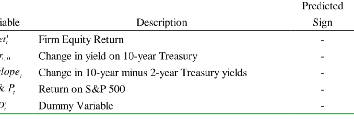
Table 1 summarizes the predicted sign of the correlation between changes in credit spreads and changes in the underlying variable. The variable i
t
ret is firm equity
return with predicted negative correlation. The variable∆rt,10is change in yield on 10-year Treasury with predicted negative correlation. The variable∆slopetis change in 10-year minus 2-year Treasury yields with predicted negative correlation. The
variableS &Ptis return on S&P 500 with predicted negative correlation. The variableDtiis dummy variable with predicted negative correlation.
Table 2 summarizes the descriptive statistics of credit spreads which are divided into two parts, before and after switching. We use data at a disaggregated level making a distinction between credit spreads for two parts and six maturity classes to examine the mean, median, std. deviation, minimum, maximum of credit spreads from 1998 through 2003 at a daily frequency.
Table 1
Explanatory Variables and Expected Signs on the Coefficients of the Regression:
i t i t i t i t i t i t i i t i i t ret r r slope S P D CS =α+β1 +β2∆ ,10 +β3(∆ ,10)2 +β4∆ +β5 & +β6 +ε Variable Description Predicted Sign i t
ret Firm Equity Return -
10 ,
t
r
∆ Change in yield on 10-year Treasury -
t
slope
∆ Change in 10-year minus 2-year Treasury yields -
t
P
S & Return on S&P 500 -
i t
Table 2
Descriptive statistics of credit spreads are divided into two parts, before and after switching:
Statistics
Mean Median Std. Deviation Minimum Maximum
(before) (after) (before) (after) (before) (after) (before) (after) (before) (after) Two — 0.198474 — 0.083 — 0.350827 — -0.6151 — 1.596 Three — 0.192596 — 0.008 — 0.594643 — -1.724 — 1.933 Five 0.62706 0.364869 0.92545 0.1494 1.83581 1.27283 -4.7226 -53.4798 7.0579 24.1023 Seven 0.592335 0.889905 0.4355 0.1474 1.512808 8.38908 -7.6332 -15.678 14.547 902.4448 Ten 1.529869 3.350785 0.9692 0.9724 3.749798 237.5509 -3.5952 -4.2016 519.472 48329.44 Thirty 1.118936 1.863425 0.962 1.7406 0.824494 1.328071 -4.7017 -4.8529 5.327 8.7485
4. Empirical Results
The credit spread CS (t) is defined as CS (t)= CS (Vt , rt ,
{ }
Xt ), where V is firm value, r is the spot rate, and{ }
Xt represents all of the other “state variables” used for specifying the model (see Collin-Dufresne, Goldstein, and Martin (2001)). Since credit spreads are determined given the current values of the state variables, it follows that structural models generate predictions for what the theoretical determinants of credit spreads should be, and moreover offer a prediction for whether changes in these variables should be positively or negatively correlated with credit spreads. Inaccordance with the proxies for explanatory variables of credit spreads, each determinant is discussed individually.
The tables below report OLS estimates of the regression, and summary statistics of the distribution of coefficient estimates are presented. Table 3 shows the integrated data table of individual firm’s time series regression, and summarizes the estimation coefficients and the p-values of explanatory variables in the time-series regression for 34 switching firms. Permanent code (PERMCO) of 34 firms refer to appendix. Table 4 summarizes the estimation coefficients and p-values of explanatory variables in the cross-sectional regression at each firm’s switching date. We use 5% significant level. If p-value is less than 0.05, there is statistically significant relation between credit spread and the variables introduced above.
Most of the variables investigated in the regressions have some ability to explain changes in credit spreads. Further, the signs of the estimated coefficients generally agree with theory.
From Table 3, the firm equity return i t
ret is with predicted negative sign, but not statistically significant, for most (almost 91%) firms in the multivariate analyses. Indeed, the factor loading on the S&P 500 return is typically several times larger than the loading on the firm’s own equity return. This is the first indication that daily
Table 3
Estimation Coefficients of Explanatory Variables of the Time-Series Regression: For individual
bond i of 34 firms with credit spread i t
CS over the period January 1998 to December 2003, we estimate
the following regression: i
t i t i t i t i t i t i i t i i t ret r r slope S P D CS =α+β +β ∆ +β ∆ +β4∆ +β5 +β6 +ε 2 10 , 3 10 , 2 1 ( ) & Note:
Figures in the upper rows of variables indicate coefficients, and figures in ( ) indicate their p-values. Variable PERMCO retti 10 t r ∆ 10 2 ) (∆rt ∆slopet S &Pt i t D 4521 -0.655311 (0.0447)** -0.255523 (0.0731)* 0.315343 (0.8077) -0.095941 (0.0000)*** -0.824065 (0.2496) -0.390127 (0.0000)*** 11108 -1.003842 (0.0182)** -0.178302 (0.5244) 4.120822 (0.0981)* -0.458060 (0.0000)*** -0.446828 (0.7531) -2.960317 (0.0000)*** 2381 -0.061292 (0.9035) -0.342085 (0.0203)** -0.581783 (0.6698) 0.451428 (0.0000)*** -1.383366 (0.0443)** -0.287029 (0.0000)*** 16061 -0.007279 (0.0029)*** -1.279810 (0.0784)* -13.78461 (0.0928)* 2.688810 (0.0000)*** -1.085748 (0.7105) -1.176969 (0.0000)*** 22031 -1.894951 (0.3611) -0.643887 (0.6305) 14.98827 (0.2025) 1.777131 (0.0000)*** -4.460996 (0.5608) -3.484373 (0.0000)*** 5651 -0.805781 (0.2313) -0.043372 (0.9286) 9.289033 (0.0413)** -0.149044 (0.0000)*** -0.450778 (0.8434) -0.961356 (0.0000)*** 14237 -0.010355 (0.3452) -0.278667 (0.7503) 11.39779 (0.2770) -5.550929 (0.0000)*** -2.625212 (0.5562) -1.040966 (0.0000)*** 13665 -13.21044 (0.6509) -11.84481 (0.8607) 388.0689 (0.4972) -187.6909 (0.0000)*** -462.9410 (0.0749)* -75.01070 (0.0000)*** 15602 -12.13866 (0.0002)*** -3.675929 (0.2726) 106.2136 (0.0007)*** -2.062926 (0.0145)** -13.68298 (0.4334) -10.52311 (0.0000)*** 2589 -0.652810 (0.8178) -1.356061 (0.3181) -9.980395 (0.3682) -1.813234 (0.0007)*** -0.525127 (0.9482) -5.958353 (0.0000)*** 2801 -0.099259 (0.7500) -0.418296 (0.0000)*** 2.360247 (0.0046)*** 0.072286 (0.0000)*** -0.865748 (0.0396)** -0.563111 (0.0000)*** 12318 -3.740239 (0.4824) -1.642038 (0.7778) -32.01164 (0.5653) 13.19793 (0.0000)*** -1.993312 (0.9331) -6.547389 (0.0000)*** 15946 -0.329215 (0.9183) -1.091962 (0.7240) 100.1578 (0.0017)*** -2.104894 (0.0364)** -22.82828 (0.0598)* -1.023206 (0.0135)** 9662 0.073043 (0.9109) -0.305453 (0.2558) -2.308288 (0.3365) 1.693512 (0.0000)*** -1.212264 (0.4136) -0.399391 (0.0000)*** 15545 -0.002775 (0.8448) -0.017007 (0.9609) 8.281434 (0.0166)** 1.613494 (0.0000)*** -0.325332 (0.8317) -0.115407 (0.0123)** 3306 -0.308195 -0.310802 1.396296 0.203844 -0.923668 -0.592285
(0.4545) (0.0051)*** (0.1759) (0.0000)*** (0.0892)* (0.0000)*** 5238 -0.554699 (0.4116) -0.623574 (0.0615)* 7.853321 (0.0086)*** 0.100903 (0.0013)*** -0.391316 (0.8057) -0.452398 (0.0000)*** 11070 -0.132386 (0.8587) -0.220789 (0.5712) 2.312423 (0.5123) 0.243813 (0.0000)*** -0.224246 (0.9056) -0.730106 (0.0000)*** 32056 -0.010063 (0.1608) -0.276256 (0.1153) 0.256787 (0.8772) -0.355753 (0.0000)*** -0.367927 (0.6521) -1.534557 (0.0000)*** 14915 -4.471458 (0.2998) -1.578867 (0.5786) -25.57000 (0.3219) -1.920075 (0.0000)*** -23.91885 (0.1362) -11.06217 (0.0000)*** 16268 -2.828522 (0.1522) -1.428096 (0.3361) -7.093392 (0.6087) -1.833114 (0.0000)*** -3.835661 (0.6282) -7.699108 (0.0000)*** 17927 -1.634623 (0.6332) -15.54375 (0.0013)*** 119.6268 (0.0159)** 2.478028 (0.0000)*** -9.161650 (0.6629) -2.794500 (0.0036)*** 6959 0.054605 (0.9565) -0.099826 (0.8261) 0.167400 (0.9651) -0.253459 (0.0340)** -2.739742 (0.2880) -1.149146 (0.0000)*** 11735 -0.748626 (0.0075)*** -0.086811 (0.7155) 8.661405 (0.0001)*** 1.483341 (0.0000)*** -0.626670 (0.5838) -0.179802 (0.0005)*** 15961 -6.760593 (0.0000)*** -0.421655 (0.6613) 8.981914 (0.2652) 0.031911 (0.8195) -2.434223 (0.6078) -4.414141 (0.0000)*** 1523 -6.751421 (0.0621)* -5.345427 (0.0919)* 46.94720 (0.1640) -8.582602 (0.0000)*** -11.13392 (0.4305) -7.612228 (0.0000)*** 8782 -0.626539 (0.1923) -0.273008 (0.1779) 1.274711 (0.5484) 0.013854 (0.4967) -1.083500 (0.2937) -1.190992 (0.0000)*** 11857 -1.038704 (0.2991) -0.763778 (0.0361)** 2.399365 (0.4957) 0.522031 (0.0004)*** -0.144656 (0.9279) -0.527809 (0.0000)*** 7558 1.156306 (0.6752) -0.905226 (0.5851) -16.62551 (0.2415) 0.312814 (0.6450) -5.960221 (0.5182) -2.103284 (0.0000)*** 1718 -0.284562 (0.5250) -0.265119 (0.0654)* 1.234463 (0.3060) -0.414228 (0.0000)*** -0.530485 (0.4951) -0.632999 (0.0000)*** 12007 -1.921404 (0.4030) -1.549813 (0.2569) -4.120985 (0.7672) -0.146276 (0.8103) -7.356438 (0.4434) -7.198410 (0.0000)*** 2510 -3.432860 (0.1049) -0.298105 (0.5577) 0.872629 (0.8559) -0.461800 (0.4062) -2.379282 (0.7082) -0.140510 (0.2155) 11418 -11.13956 (0.0312)** -0.526205 (0.8178) 11.64840 (0.5749) 1.704753 (0.0000)*** -9.703993 (0.3958) -0.299097 (0.5101) 41465 -2.148436 (0.2370) -1.197619 (0.0921)* 9.533713 (0.2521) -2.134763 (0.0000)*** -0.411941 (0.9415) -0.100361 (0.6553) Average -2.29767370 -1.6202332 22.243631 -5.5128857 -17.617042 -4.7310502
changes in firm-specific attributes are not the driving force in credit spread changes (Collin-Dufresne, Goldstein, and Martin (2001)). Then, Collin-Dufresne, Goldstein, and Martin (2001) also demonstrate that the apparently weak explanatory power of firm-specific variables is not due to potential collinearity with the market return S&Pt.
We expect a negative relation between the risk-free rate and the credit spread. The drift of the risk-neutral process of the value of the assets, which is the expected growth of the firm’s asset value, equals the risk-free interest rate. An increase in the interest rate implies an increase in the expected growth rate of the firm’s asset value. This will in turn reduce the probability of default and the credit spread (see Longstaff and Schwartz (1995)). This prediction is borne out in their data. Further evidence is provided by Duffee (1998), who uses a sample restricted to noncallable bonds and finds a significant, albeit weaker, negative relationship between changes in credit spreads and interest rates. Furthermore, lower interest rates are usually associated with a weakening economy and thus higher credit spreads.
Our result is consistent with the empirical findings of Longstaff and Schwartz (1995) and Duffee (1998), we find that an increase in the risk-free rate lowers the credit spread for all bonds. Once again, this finding can be explained by noting that an increase in drift decreases the risk-neutral probability of default, and that the closer firms are to the default threshold, the more sensitive they are to this change.
The expectations hypothesis of the term structure implies that the slope of the default-free term structure (the Treasury yield curve slope), which is often measured as the spread between the long-term and the short-term rate, is an optimal predictor of future changes in short-term rates over the life of the long-term bond. As such, an increase in the slope implies an increase in the expected short-term interest rates. As in the case of the motivation for the risk-free interest rate above, it should also lead to a decrease in credit spreads. Although the spot rate is the only interest-rate-sensitive
factor that appears in the firm value process, the spot rate process itself may depend upon other factors as well. For example, Litterman and Scheinkman (1991) and Chen and Scott (1993) find that the two most important factors driving the term structure of interest rates are the level and slope of the term structure. Furthermore, the slope of the term structure is often related to future business cycle conditions (see, for example, Estrella and Hardouvelis (1991), Bernard and Gerlach (1998), and Estrella and
Mishkin (1995, 1998)). A decrease in the slope is considered to be indicators of a weakening economy. It is reasonable to believe that the expected recovery rate might decrease in times of recession. A positively sloped yield curve is associated with improving economic activity, which might in turn increase a firm’s growth rate and reduce its default probability. This strengthens our expectations of a negative relation between the slope and the credit spread.
Overall, convexity of the term structure is not significant statistically. Slope of the term structure is statistically significant for 44% firms in the multivariate analyses only. As expected, it has a negative impact for half firms in the multivariate analyses.
Even if the probability of default remains constant for a firm, changes in credit spreads can occur due to changes in the expected recovery rate. The expected recovery rate in turn should be a function of the overall business climate (Collin-Dufresne, Goldstein, and Martin (2001)).
The return of the S&P 500 is insignificant statistically. Estimated coefficients have the same sign for all firms. As expected, it has a negative impact.
Generally speaking, listing increases a firm’s visibility through announcements and receives more attention from financial analysts and investors. Moreover, listing on the national exchange, especially on the NYSE, is considered a prestigious milestone in corporate development. Additionally, because the criteria for listing on the NYSE are more stringent than those on the AMEX or the NASDAQ, switching
firms that meet the criteria have been considered a positive signal about their future prospects. Accordingly, it is reasonable to assume that risks of switching firms would somehow been decreased.
In the time-series regressions of a sample of 235 bonds from 34 firms during the period 1998 - 2003, the dummy variable, i
t
D , is statistically significant for 91% firms in the multivariate analyses. The sign, as expected, indicates that after these firms switch to NYSE, which has stricter restriction of listing, triggers a decrease in credit spreads. The behavior is relatively homogeneous across all firms.
Table 4 summarizes the estimation coefficients and p-values of explanatory variables in the cross-sectional regression at each firm’s switching date.
As in the case of the motivation for the time-series regressions above, in the cross-sectional regression, the dummy variable is statistically insignificant at 5% significant level. The evidence also proves that whether a company moves from the NASDAQ to the NYSE or from the AMEX to the NYSE, the effects on credit spreads are similar, no matter which exchange the switching originated from due to both groups listing on the same exchange.
Table 4
Estimation Coefficients and P-Values of Explanatory Variables of the Cross-Sectional Regression:
For each sample bond i at date t with credit spread i t
CS over the period January 1998 to
December 2003, the following regression is assumed:
i t i t i t i t i t i t i i t i i t ret r r slope S P D CS =α +β1 +β2∆ ,10 +β3(∆ ,10)2 +β4∆ +β5 & +β6 +ε
t is exchange date for each firm.
Variable Coefficient Std. Error t-Statistic Prob. EQUITY_RETURN -5.828633 3.015136 -1.933124 0.0552* DR10 -1.900905 4.476551 -0.424636 0.6717 DR10_2 103.4797 45.36812 2.280890 0.0240** R10_R2 -0.217467 0.235489 -0.923474 0.3573 S_P_RETURN -7.863237 15.70653 -0.500635 0.6174 DUMMY -0.273481 1.505869 -0.181610 0.8561 C 2.430080 1.434022 1.694590 0.0923* Adjusted R-squared 0.023484 R-squared 0.062807 Log likelihood -335.9307 F-statistic 1.597204 Durbin-Watson stat 1.562411 Prob(F-statistic) 0.152089 Note: White Heteroskedasticity-Consistent Standard Errors & Covariance
5. Conclusions
In this paper, we mainly analyze whether the sensitivity of credit spread changes to the firms that switch their locations is significant. Using data of 34 firms that switched from the American Stock Exchange (AMEX) to the New York Stock Exchange (NYSE) and from the National Association of Securities Dealers’
Automated Quotations system (NASDAQ) to the NYSE during the period 1998 -2003, we first examine the changes in credit spreads of individual 34 firms that switching to NYSE by adopting a multivariate time-series regression approach. The regression also includes several economic and financial variables to capture effects of determinants on credit spreads changes.
First, we find the dummy variable is statistically significant for almost all firms in the multivariate analyses. The sign, as expected, indicates that after these firms switch to NYSE, which has stricter restriction of listing, triggers a decrease in credit spreads. Second, we find the firm equity return is negative for most firms in the multivariate analyses. It is consistent with the results of Collin-Dufresne, Goldstein, and Martin (2001). Third, we find that an increase in the risk-free rate lowers the credit spread for all bonds. It is consistent with the empirical findings of Longstaff and Schwartz (1995) and Duffee (1998). Fourth, the slope of the term structure is statistically significant for most firms in the multivariate analyses. As expected, it has a negative impact. Fifth, the estimated coefficients of the return of the S&P 500 have the same sign for all firms. As expected, it has a negative impact.
Finally, we analyze if there exists difference between switching of two situations, from the NASDAQ to the NYSE and from the AMEX to the NYSE. In the
cross-sectional regression, the dummy variable is statistically insignificant. The evidence indicates that there is no difference in credit spreads no matter which exchange the switching originated from. They both switch to the same terminus. This result is also intuitive.
References
1. Baker, H.K. and M.C. Johnson, 1990, “A Survey of Management Views on Exchanges Listing,” Quarterly Journal of Business and Economics 29, 3-20.
2. Bernard, H. and S. Gerlach, 1998, “Does the term structure predict recessions? The international evidence,” CEPR Discussion Paper 1892.
3. Bevan, A. and F. Garzarelli, 2000, “Corporate Bond Spreads and the Business Cycle,” The Journal of Fixed Income 9, 8-18.
4. Black, Fischer and John C. Cox, 1976, “Valuing corporate securities: Some effects of bond indentures provisions,” Journal of Finance 31, 351–367.
5. Black, F. and M. Scholes, 1973, “The Pricing of Otpions and Corporate Liabilities,” Journal of Political Economy 81, 637-59.
6. Brown, David T., 2001, “An Empirical Analysis of Credit Spread Innovations,”
Maturity and Credit Quality, working paper.
7. Chance, D., 1990, “Default risk and the duration of zero coupon bonds,” Journal of
Finance 45, 265-274.
8. Chen, R.-R. and Scott L., 1993, “Maximum likelihood estimation for a multifactor equilibrium model of the term structure of interest rates,” Journal of Fixed Income 3, 14-31.
9. Christie, William G. and Roger D. Huang, 1993, “Market structures and liquidity: A transactions data study of exchange listings,” Journal of Financial Intermediation 3, 300-326.
10. Collin-Dufresne, P., R.S. Goldstein, and J.S. Martin, 2001, “The Determinants of Credit Spread Changes,” Journal of Finance 56, 2177-2207.
11. Collin-Dufrense, P. Robert Goldstein, and J. Spencer Martin, 1999, “The
Determinants of Credit Spread Changes,” unpublished manuscript, Carnegie Mellon University.
Institutional Investor Inc., 36-48.
13. Dharan, B.G. and D.L. Ikenberry, 1995, “The long-run negative drift of post- listing stock return,” Journal of Finance 50, 1547-1574.
14. Duffee, Gregory R., 1998, “The relation between treasury yields and corporate bond yield spreads,” Journal of Finance 53, 2225–2241.
15. Duffie, Darrell, and Ken Singleton, 1999, “Modeling term structures of defaultable bonds,” Review of Financial Studies 12, 687–720.
16. Estrella, A. and Hardouvelis G. A., 1991, “The term structure as a predictor of real economic activity,” Journal of Finance 46, 555-576.
17. Estrella, A. and Mishkin F. S., 1995, “The term structure of interest rates and its role in monetary policy for the european central bank,” NBER Working Paper 5279.
18. Estrella, A. and Mishkin F. S., 1998, “Predicting U.S. recessions: Financial variables as leading indicators,” Review of Economics and Statistics 80, 45-61.
19. Geske, R, 1977, “The Valuation of Corporate Liabilities as Compound Options,”
Journal of Financial and Quantitative Analysis 12, 541-552.
20. Grammatikos, T. and G. J. Papaioannou, 1986, “Market reaction to NYSE listings: Tests of the marketability gains hypothesis,” Journal of Financial Research 9,
215–27.
21. Ho, T. and R. Singer, 1982, “Bond indenture provisions and the risk of corporate debt,” Journal of Financial Economics 10, 375-406.
22. Ho, T. and R. Singer, 1984, “The value of corporate debt with a sinking fund provision,” Journal of Business 57, 315-336.
23. Houweling, P., Mentink A., and Vorst, T., 2002, “How to measure corporate liquidity? ,” Tinbergen Institute Discussion Paper 030/02.
24. Hull, J and A White, 2000, “Valuing credit default swaps,” two parts, working paper.
25. Hwang, Chuan-Yang and Narayanan Jayaraman, 1993, “The Post-listing Puzzle: evidence from Tokyo Stock Exchange Listings,” Pacific-Basin Finance Journal 1, 111-126.
26. Ikenberry, D., Lakonishok J., and Vermaelen, T., 1995, “Market underreaction to open market share repurchases,” Journal of Financial Economics 39, 181-208.
27. Jarrow, Robert A., and Stuart Turnbull, 1995, “Pricing derivatives on financial securities subject to credit risk,” Journal of Finance 50, 53–86.
28. Johnson, H. and R. Stulz, 1987, “The pricing of options with default risk,”
Journal of Finance 42, 267-280.
29. Jones, E. Philip, Scott P. Mason, and Eric Rosenfeld, 1984, “Contingent Claims Analysis of Corporate Capital Structure:An Empirical Investigation,” Journal of
Finance 39, 611-625.
30. Kaldec, B.G. and J.J. McConnell, 1994, “The effect of market segmentation and liquidity on asset price: Evidence from exchange listings,” Journal of Finance 49, 611-636.
31. Kim, In Joon, Krishna Ramaswamy, and Suresh Sundaresan, 1993, “Does default risk in coupons affect the valuation of corporate bonds? A contingent claims model,”
Financial Management 22, 117–131.
32. Leland, H E, 1994, “Corporate debt value, bond covenants, and optimal capital structure,” Journal of Finance 49, 1213-52.
33. Leland, H E and K B Toft, 1996, “Optimal capital structure, endogenous bankruptcy, and the term structure of credit spreads,” Journal of Finance 51, 987-1019.
34. Litterman, Robert and Jose Scheinkman, 1991, “Common factors affecting bond returns,” Journal of Fixed Income 1, 54–61.
35. Longstaff, Francis and Eduardo Schwarts, 1995, “A Simple Approach To Valuing Risky Fixed and Floating Rate Debt,” Journal of Finance 50, 789-819.
36. Loughran, T. and J. Ritter, 1995, “The new issues puzzle,” Journal of
Finance 50, 23-51.
37. Madan, D and H Unal, 1999, “A two-factor hazard-rate model for pricing risky debt and the term structure of credit spreads,” University of Maryland Working Paper.
38. Masazumi, Hattori, Koji Koyama, and Tatsuya Yonetani, 2001,“Analysis of Credit Spread in Japan’s Corporate Bond Market,” www.bis.com. in BIS Paper No 5.
39. McConnell, J.J. and G.C. Sanger, 1987, “The puzzle post-listing common stock return,” Journal of Finance 42, 119-140.
40. McConnell, J.J. and G. C. Sanger, 1984, “A trading strategy for listings on the NYSE,” Financial Analysis Journal 40, 34-38.
41. Merton, Robert C., 1977, “On the Pricing of Contingent Claims and The Modigliani-Miller theorem,” Journal of Financial Economics 5, 241-249.
42. Merton, Robert C., 1974, “On The Pricing of Corporate Debt: The Risk structure of Interest Rates,” Journal of Finance, 449-470.
43. Mikkelson, W. H. and K. Shah, 1994, “Performance of companies around initial public offerings,” Working paper, University of Oregon.
44. Morris, C., R. Neale, and D. Rolph, 1998, “Credit Spreads and Interest Rates: A Cointegration Approach,” Working paper, Federal Reserve Bank of Kansas City.
45. Nelson, William R., 1994, “Do firms buy low and sell high? Evidence of excess returns on firms that issue or repurchase equity,” Working paper, Federal Reserve Board.
46. Perraudin, W. R. and Taylor A. P., 2003, “Liquidity and bond market spreads,”
EFA2003 Annual Conference no. 879.
47. Ramaswamy, K., and S. Sundaresan, 1986, “The valuation of floating-rate instruments,” Journal of Financial Economics 17, 251-272.
48. Ronn, E. I. and Verma A. K., 1986, “Pricing risk-adjusted deposit insurance: An option-based model,” Journal of Finance 41, 871-895.
49. Sanger, G. C. and J.J. McConnell, 1986, “Stock exchange listings, firm value, and security market efficiency: The impact of Nasdaq,” Journal of Finance and
Quantitative Analysis 21, 1-25.
50. Spiess, D.K. and J. Affleck-Graves, 1995, “Underperformance in long-run stock return following seasoned equity offerings,” Journal of Finance Economics 38, 243-267.
51. Ule, Maxwell G., 1937, “Price movements of newly listed common stock,”
Journal of Business 10, 346-369.
52. Van Horne, J. C., 1970, “New listings and their price behavior,” Journal of
Finance 25, 783-749.
53. Ying, L. K. W. and W. G. Lewellen, G. G. Schlarbaum and R. C. Lease, 1977, “Stock exchange listing and securities return,” Journal of Financial and Analysis 12, 415-432.
Appendix
Table 1
Table 2
Company Name: ALLIED WASTE INDUSTRIES INC (11108) Variable Coefficient Std. Error t-Statistic Prob. EQUITY_RETURN -1.003842 0.425169 -2.361041 0.0182** DR10 -0.178302 0.280097 -0.636573 0.5244 DR10_2 4.120822 2.490700 1.654483 0.0981* R10_R2 -0.458060 0.020632 -22.20114 0.0000*** S_P_RETURN -0.446828 1.420168 -0.314630 0.7531 DUMMY -2.960317 0.036855 -80.32400 0.0000*** C 1.497497 0.026532 56.44123 0.0000*** R-squared 0.456632 Durbin-Watson stat 0.020086 Adjusted R-squared 0.456225 F-statistic 1121.059 Log likelihood -14402.55 Prob(F-statistic) 0.000000
Company Name: TOYOTA MOTOR CORP (4521)
Variable Coefficient Std. Error t-Statistic Prob. EQUITY_RETURN -0.655311 0.326475 -2.007233 0.0447** DR10 -0.255523 0.142587 -1.792045 0.0731* DR10_2 0.315343 1.295599 0.243396 0.8077 R10_R2 -0.095941 0.010552 -9.092572 0.0000*** S_P_RETURN -0.824065 0.715737 -1.151351 0.2496 DUMMY -0.390127 0.030990 -12.58877 0.0000*** C 0.384637 0.025544 15.05807 0.0000*** R-squared 0.009876 Durbin-Watson stat 0.010625 Adjusted R-squared 0.009556 F-statistic 30.83773 Log likelihood -29452.09 Prob(F-statistic) 0.000000
Table 3
Company Name: ENBRIDGE INC (2381)
Variable Coefficient Std. Error t-Statistic Prob. EQUITY_RETURN -0.061292 0.505363 -0.121283 0.9035 DR10 -0.342085 0.147431 -2.320311 0.0203** DR10_2 -0.581783 1.364270 -0.426443 0.6698 R10_R2 0.451428 0.019426 23.23867 0.0000*** S_P_RETURN -1.383366 0.687918 -2.010948 0.0443** DUMMY -0.287029 0.039699 -7.230131 0.0000*** C 1.470314 0.014307 102.7662 0.0000*** R-squared 0.030457 Durbin-Watson stat 0.004895 Adjusted R-squared 0.030333 F-statistic 245.0523 Log likelihood -96660.94 Prob(F-statistic) 0.000000
Table 4
Company Name: S F X ENTERTAINMENT INC (16061) Variable Coefficient Std. Error t-Statistic Prob. EQUITY_RETURN -0.007279 0.002389 -3.046574 0.0029*** DR10 -1.279810 0.720358 -1.776631 0.0784* DR10_2 -13.78461 8.127695 -1.696005 0.0928* R10_R2 2.688810 0.151199 17.78325 0.0000*** S_P_RETURN -1.085748 2.917725 -0.372121 0.7105 DUMMY -1.176969 0.064988 -18.11043 0.0000*** C 3.167933 0.045031 70.34931 0.0000*** Adjusted R-squared 0.878483 R-squared 0.884879 Log likelihood -21.08617 F-statistic 138.3567 Durbin-Watson stat 0.707395 Prob(F-statistic) 0.000000
Table 5
Company Name: ALARIS MEDICAL SYSTEMS INC (22031) Variable Coefficient Std. Error t-Statistic Prob. EQUITY_RETURN -1.894951 2.073616 -0.913839 0.3611 DR10 -0.643887 1.337969 -0.481242 0.6305 DR10_2 14.98827 11.75204 1.275377 0.2025 R10_R2 1.777131 0.273725 6.492395 0.0000*** S_P_RETURN -4.460996 7.665960 -0.581923 0.5608 DUMMY -3.484373 0.218063 -15.97877 0.0000*** C -1.314353 0.571143 -2.301268 0.0216** Adjusted R-squared 0.378078 R-squared 0.382266
Log likelihood -2100.835 F-statistic 91.27609 Durbin-Watson stat 0.012422 Prob(F-statistic) 0.000000
Table 6
Company Name: N B T Y INC (5651)
Variable Coefficient Std. Error t-Statistic Prob. EQUITY_RETURN -0.805781 0.672869 -1.197531 0.2313 DR10 -0.043372 0.483863 -0.089637 0.9286 DR10_2 9.289033 4.547345 2.042737 0.0413** R10_R2 -0.149044 0.030512 -4.884786 0.0000*** S_P_RETURN -0.450778 2.281521 -0.197578 0.8434 DUMMY -0.961356 0.141638 -6.787442 0.0000*** C 4.627431 0.042271 109.4693 0.0000*** Adjusted R-squared 0.063696 R-squared 0.067494 Log likelihood -2243.983 F-statistic 17.76907 Durbin-Watson stat 0.025271 Prob(F-statistic) 0.000000
Table 7
Company Name: STAR GAS PARTNERS LP (14237) Variable Coefficient Std. Error t-Statistic Prob. EQUITY_RETURN -0.010355 0.010953 -0.945356 0.3452 DR10 -0.278667 0.874999 -0.318476 0.7503 DR10_2 11.39779 10.46599 1.089032 0.2770 R10_R2 -5.550929 0.196227 -28.28825 0.0000*** S_P_RETURN -2.625212 4.456374 -0.589092 0.5562 DUMMY -1.040966 0.126032 -8.259572 0.0000*** C 7.525547 0.086330 87.17148 0.0000*** Adjusted R-squared 0.728185 R-squared 0.733363 Log likelihood -341.5032 F-statistic 141.6464 Durbin-Watson stat 0.242723 Prob(F-statistic) 0.000000
Table 8
Company Name: C H S ELECTRONICS INC (13665) Variable Coefficient Std. Error t-Statistic Prob. EQUITY_RETURN -13.21044 29.12582 -0.453565 0.6509 DR10 -11.84481 67.37280 -0.175810 0.8607 DR10_2 388.0689 569.9702 0.680858 0.4972 R10_R2 -187.6909 22.11034 -8.488827 0.0000*** S_P_RETURN -462.9410 257.7753 -1.795909 0.0749* DUMMY -75.01070 15.58657 -4.812520 0.0000*** C 14.06040 14.51335 0.968791 0.3345 Adjusted R-squared 0.371447 R-squared 0.399591
Log likelihood -696.3906 F-statistic 14.19803 Durbin-Watson stat 0.157216 Prob(F-statistic) 0.000000
Table 9
Company Name: FRIEDE GOLDMAN INTERNATIONAL INC (15602) Variable Coefficient Std. Error t-Statistic Prob. EQUITY_RETURN -12.13866 3.208178 -3.783662 0.0002*** DR10 -3.675929 3.342856 -1.099637 0.2726 DR10_2 106.2136 30.91533 3.435628 0.0007*** R10_R2 -2.062926 0.837010 -2.464638 0.0145** S_P_RETURN -13.68298 17.43658 -0.784728 0.4334 DUMMY -10.52311 0.374335 -28.11146 0.0000*** C 2.914086 0.308007 9.461089 0.0000*** Adjusted R-squared 0.788079 R-squared 0.793513 Log likelihood -570.7901 F-statistic 146.0310 Durbin-Watson stat 0.317837 Prob(F-statistic) 0.000000
Table 10
Company Name: K V PHARMACEUTICAL CO (2589) Variable Coefficient Std. Error t-Statistic Prob. EQUITY_RETURN -0.652810 2.832557 -0.230467 0.8178 DR10 -1.356061 1.357575 -0.998884 0.3181 DR10_2 -9.980395 11.08418 -0.900418 0.3682 R10_R2 -1.813234 0.530024 -3.421043 0.0007*** S_P_RETURN -0.525127 8.083427 -0.064963 0.9482 DUMMY -5.958353 0.996725 -5.977933 0.0000*** C 2.546704 0.287756 8.850236 0.0000*** Adjusted R-squared 0.239881 R-squared 0.245409 Log likelihood -1861.288 F-statistic 44.39272 Durbin-Watson stat 0.024027 Prob(F-statistic) 0.000000
Table 11
Company Name: MCCORMICK & CO INC (2801)
Variable Coefficient Std. Error t-Statistic Prob. EQUITY_RETURN -0.099259 0.311532 -0.318615 0.7500 DR10 -0.418296 0.087483 -4.781472 0.0000*** DR10_2 2.360247 0.833533 2.831617 0.0046*** R10_R2 0.072286 0.006147 11.75989 0.0000*** S_P_RETURN -0.865748 0.420767 -2.057548 0.0396** DUMMY -0.563111 0.012309 -45.74971 0.0000*** C 1.237294 0.009276 133.3888 0.0000*** Adjusted R-squared 0.131800 R-squared 0.132018 Log likelihood -28282.82 F-statistic 604.4378 Durbin-Watson stat 0.032057 Prob(F-statistic) 0.000000
Table 12
Company Name: WESTPOINT STEVENS INC (12318) Variable Coefficient Std. Error t-Statistic Prob. EQUITY_RETURN -3.740239 5.319494 -0.703119 0.4824 DR10 -1.642038 5.816522 -0.282306 0.7778 DR10_2 -32.01164 55.62536 -0.575486 0.5653 R10_R2 13.19793 0.393185 33.56673 0.0000*** S_P_RETURN -1.993312 23.73935 -0.083967 0.9331 DUMMY -6.547389 0.777846 -8.417336 0.0000*** C 0.181561 0.675547 0.268762 0.7882 Adjusted R-squared 0.771356 R-squared 0.774577
Log likelihood -1431.645 F-statistic 240.5271 Durbin-Watson stat 0.238519 Prob(F-statistic) 0.000000
Table 13
Company Name: GLOBAL TELESYSTEMS GRP INC (15946) Variable Coefficient Std. Error t-Statistic Prob. EQUITY_RETURN -0.329215 3.202537 -0.102798 0.9183 DR10 -1.091962 3.086766 -0.353756 0.7240 DR10_2 100.1578 31.44124 3.185555 0.0017*** R10_R2 -2.104894 0.997571 -2.110020 0.0364** S_P_RETURN -22.82828 12.04029 -1.895991 0.0598* DUMMY -1.023206 0.409343 -2.499633 0.0135** C 5.144349 0.248645 20.68956 0.0000*** Adjusted R-squared 0.122637 R-squared 0.154736 Log likelihood -352.1071 F-statistic 4.820629 Durbin-Watson stat 0.398988 Prob(F-statistic) 0.000152
Table 14
Company Name: CHARTER ONE FINANCIAL INC (9662) Variable Coefficient Std. Error t-Statistic Prob. EQUITY_RETURN 0.073043 0.652287 0.111980 0.9109 DR10 -0.305453 0.268605 -1.137182 0.2558 DR10_2 -2.308288 2.400227 -0.961695 0.3365 R10_R2 1.693512 0.072804 23.26121 0.0000*** S_P_RETURN -1.212264 1.481856 -0.818072 0.4136 DUMMY -0.399391 0.062597 -6.380337 0.0000*** C 1.193801 0.030446 39.21012 0.0000*** Adjusted R-squared 0.395952 R-squared 0.400377 Log likelihood -439.0656 F-statistic 90.47527 Durbin-Watson stat 0.063728 Prob(F-statistic) 0.000000