在推廣的Vasicek模型下的可違約債定價

國

立

交

通

大

學

應用數學系

碩

士

論

文

在推廣的 Vasicek 模型下的可違約債定價

Price Default Bonds Under The Generalized Vasicek Model

研 究 生：張嘉文

指導教授：許元春 教授

在推廣的 Vasicek 模型下的可違約債定價

學生：

張嘉文

指導教授

：許元春

國立交通大學應用數學學系﹙研究所﹚碩士班

摘

要

本論文將以推廣的 Vasicek 模型假設利率以及可違約債違約的彈性，

再用 ITO’s Formula 來對可違約債作定價，求出推廣的 Vasicek 的各

項參數，藉此來對各筆可違約債的評價，給一些數量化的解釋，以期

往後能夠找出更合適的數據，給出一個公司合理的信用評等。

Price Default Bonds

Under The Generalized Vasicek Model

student：

Chia-Wen Chang

Advisors：Dr.

Yuan-Chung Sheu

Department﹙Institute﹚of

Applied Mathematics

National Chiao Tung University

ABSTRACT

In this paper, we will use the technique of the Ito’s Formula to price the

defaultbond. The interest rate model is a special case of the generalized

Vasicek model. In addition, we will also introduce a way to grade the

default bonds.

誌

謝

研究所這幾年承蒙指導教授許老師元春諄諄不捨，耐心指導，獲

益良多，當完兵後希望自己也能進步，繼續向許老師請教；在學期間，

受到李章益學長以及張明淇學長的大力幫助跟細心講解，跟李孟育學

長請教 Matlab 程式，以及陳偉國、莊晉國、陳與庭、蔡明耀、胡世

謙、林詩珊、蕭雅駿等同儕提攜討論，只能以感激不盡來形容；希望

有朝一日，也能幫助以上這些一起熬過這幾年的好朋友。

iii

目

錄

中文提要

………

i

英文提要

………

ii

誌謝

………

iii

目錄

………

iv

圖目錄

………

v

一、

緒論………

1

二、

無套利機會下，以 PDE 求價格的論證………

3

2.1

舉例………

4

2.2

推廣的 Vasicek 利率模型………

5

三、

對可違約債定價的理論與假設………

6

四、

程式模擬及市場實證………

9

五、

結論與可改進的建議………

13

參考文獻

………

14

iv

圖 目 錄

圖一

彈性

λ

及獲利率 r 為獨立情況下估計的 的比較

b

11

圖二

彈性

λ

及獲利率 r 為獨立情況下估計的

σ

的比較

11

圖三

彈性

λ

及獲利率 r 為相關情況下估計的 的比較

b

12

圖四

彈性

λ

及獲利率 r 為相關情況下估計的

σ

的比較

12

圖五

實例：負的獲利率是很常見的

13

v

PRICE DEFAULT BONDS

UNDER THE GENERALIZED VASICEK MODEL

CHIA-WEN CHANG

Abstract. In this paper, we will use the technique of the Ito’s Formula to price the default bond. The interest rate model is a special case of the gener-alized Vasicek model. In addition, we will also introduce a way to grade the default bonds.

1. Introduction

Bonds plays a very important roles in finance, whether in practice or in theory. As we consider a strategy to invest in some financial markets, we will always assume that there exists a risk-less interest rate such that we can invest the capital to it. In practice, investors usually carry out this procedure by depositing their capital in some large-scale banks. But if we hope that our strategy can be beyond reproach, then the interest rates we invest should be risk-less as possible. Hence, the treasury bonds may be the best choice for investors because the writer of these instruments is the government, Because if this reason, the treasury bonds is usually also called the default-free bond and the risk-less interest rate we earned is the discount rate. However, although the treasury bonds can be viewed as risk-less, yet, this does not mean that we can predict how much interest we earn from the bonds until the maturity because of the unpredictable changing of the bond price. This implies that as we research the phenomenon in other financial markets, the assumption that the risk-less interest rate is predictable or even constant is unreasonable if the real data of the interest rates is the discounted rates of the treasury bond in empirical studies. More and more studies have concerned the randomness of the default-free bond such that we can release the constraint if the predictable risk-less interest rate when investigating other financial markets. Recently most people have deeply believed that the mean-reverting is one of the characteristics in the literature of the inter-est rate. O. Vasicek(1997) assume that the discounted rates follows an Ornstein-Uhlenbeck process

drt= a(¯r − rt)dt + σdWt

(1.1)

where Wtis the Wiener process. In this models, O. Vasicek derive the closed form of

the bond price. In addition, F. Jamshidian(1989) has showed that the exact solution of the European call option on a U-maturity zero-coupon bond, with strike price K and expiry T ≤ U, at time t equals

Ct= P (t, U )N (h1(t, T )) − KP (t, T )N (h2(t, T ))

(1.2)

Key words and phrases. defaultable bond, pricing defaultable bond, vasicek model, extended vasicek model.

2 CHIA-WEN CHANG

where N (·) is the distribution function of the standard normal random variable and h1,2(t, T ) = log P (t, U )/P (t, T ) − log K ±1₂v2 U(t, T ) v2 U(t, T ) (1.3) v2_U(t, T ) = v 2 U(t, T ) 2a3 (1 − e −2a(T −t)_{)(1 − e}−a(U −T )₎2 (1.4)

Besides, R.R. Chen(1992) has also derived the analytical solution of the futures on default-free discounted bonds and the options on the futures. To overcome the shortcoming of the negative rate in the Vasicek model, Cox J. C., J. E. Ingersoll, and S. A. Ross(1985) suggest that the interest rate follows a square-root process

drt= a(¯r − rt)dt + σ

√ rtdWt

(1.5)

and obtain the solution of the discounted bond.

In addition to the phenomenon of the mean-reverting, researchers also admit the effect of the term structure of the interest rate. J. Hull and A. White(1990) bring up a general interest rate model which is called the Hull-White model. They assume that the interest rates follow

drt= [θ(t) + a(t)(b − r)]dt + σ(t)rβdWt

(1.6)

where θ(t) is the factor correlated to the term structure. If β is zero, the model is called the generalized Vasicek model and called the generalized CIR model if β is 1

2.

In the pricing aspect, J. Hull and A. White(2000) use a recombing trinomial tree to estimate the parameter functions which are all piecewise linear and continuous and calibrated ti market prices of the traded instruments.

In the literature of the bonds, people also concern with the price of the default-able bond. Pricing defaultdefault-able bonds is similar to price the default-free bonds. The core is still to describe the dynamics of the corresponding discounted rate. But the most difference from the default-free bond is that when we invest in the default bond, we will exposure to the default risk. Therefore, we can understand that the corresponding discounted rate will be greater than the one corresponding to the free bonds and the difference between the two rates is the default-risk-premium. This implies that if we want to price the defaultable bonds, we may be need to add additional assumption about the risk premium. Philipp J. Sch¨onbucher(2001) constructs two trinomial trees to describe the behavior of the risk-less rate and the risk premium under the assumption that the two terms are both follow the Vasicek model, and then combine the two tree together. Both the construction of the two trinomial trees are similar to the one in J. Hull and A. White(2000). As the tree has be constructed, then we can calculate the related derivative price numerically by simulations.

In this paper, we use the similar technique of the tree construction to price the credit derivatives like J. Hull and A. White(2000) and Sch¨onbucher(2001). The basic model we introduce is based on the generalized Vasicek model. Hence, our result can be viewed as the extension of Sch¨onbucher(2001). The remainders are organized as: in section II, we will review some results about the diffusion process. This part includes the derivation of the partial differential equation correlated the interest rate instruments. In section III, we will specify the theory and the assump-tions in pricing credit derivatives. In section IV, we will illustrate the empirical

PRICE DEFAULT BONDS UNDER THE GENERALIZED VASICEK MODEL 3

studies. The summary is in the last section.

2. Partial Differential Equation Derived by the No-Arbitrage Argument

In this section, we till briefly review the theory of the bond price when the dis-counted rate follows a continuous Markov process.

Let (Ω, {Ft}, P) be a probability space, and B(t,s) be the price at time t of a

zero-coupon bond maturing at time s, t ≤ s, with unit maturity value which is denoted as

B(t, s) = EP[e−Rtsr(u)du|F_t]

(2.1)

Assume the discounted interest rate follows a continuous Markov process drt= f (rt, t)dt + σ(rt, t)dWt

(2.2)

where Wtis a Wiener process under P. If the price B(t,s) is completely determined

by the assessment of the segment tτ, t ≤ τ ≤ s and the market is efficient, then by

Itˆo’s lemma

dB(t, s) = B(t, s)µ(t, s)dt − B(t, s)ρ(t, s)dWt

(2.3)

where the parameter functions are

µ(t, s) = µ(t, s, r) = 1 B(t, s, r)[Bt(t, s, r) + f Br(t, s, r) + 1 2Brr(t, s, r)] (2.4) ρ(t, s) = ρ(t, s, r) = − 1 B(t, s, r)ρBr(t, s, r) (2.5)

Now consider an investor who at time t issues an amount V1 of a bond with

maturity date s1, and simultaneously buys an amount V2 of a bond maturing at

time s2. Let V = V2− V1, then

dV = (V2µ(t, s2) − V1µ(t, s1))dt − (V2ρ(t, s2) − V1ρ(t, s1))dWt (2.6) If we choose V1 = V ρ(t, s2)/(ρ(t, s1) − ρ(t, s2)) (2.7) V2 = V ρ(t, s1)/(ρ(t, s1) − ρ(t, s2)) (2.8) then dV = V (µ(t, s2)ρ(t, s1) − µ(t, s1)ρ(t, s2)(ρ(t, s1) − ρ(t, s2))−1dt (2.9)

In addition, we assume that a loan of amount V at the discounted rate will increase in value by the increment

dV = V r(t)dt (2.10)

Compare (2.9) and (2.10), we can find that if we assume that the market is no-arbitrage, then

(µ(t, s2)ρ(t, s1) − µ(t, s1)ρ(t, s2))(ρ(t, s1) − ρ(t, s2))−1 = r(t)

(2.11)

which implies that

µ(t, s1) − r(t)

ρ(t, s1)

= µ(t, s2) − r(t) ρ(t, s2)

4 CHIA-WEN CHANG

It is worthy to note that the ratio (2.12) is independent to the maturities s1and

s2. Let

λ(t) =µ(t, s) − r(t)

ρ(t, s) s ≥ t,

(2.13)

then λ(t, r) is called the market price of risk. Writing (2.13) as µ(t, s, r) − r = λ(t, r)σ(t, s, r),

(2.14)

and substituting for µ, σ from (2.4) and (2.5), we can find that the bond price must satisfy ∂B ∂t + (f + λρ) + 1 2ρ 2∂2B ∂r2 − rB = 0 (2.15)

subject to the boundary condition

P (s, s, r) = 1 (2.16)

2.1. Example

. Vasicek(1977) considers the case that

drt= a(b − rt)dt + σdWt

(2.17)

where a, b and σ are positive constants. Under the assumption that the market price of risk λ(t, r) = λ which is a constant, the price of the bond has an analytic solution. B(t, s, r) = exp[1 a(1 − e −a(s−t)_{)(R(∞) − r) − (s − t)R(∞)} (2.18) −σ 2 4a3(1 − e −a(s−t)2 )] where R(∞) = b + σλ/a −1 2σ 2_/a2 (2.19)

can be explained as the yield for the bond with ∞-maturity.

Cox.J. C., J. E. Ingersoll and S. A. Ross(1985) consider another diffusion process which is called CIR model,

drt= a(b − rt)dt + σ

√ rtdWt

(2.20)

The most difference from the Vasicek model is that the interest rate in CIR model will not be negative, but one in the Vasicek model is not. In addition, the bond price is

B(t, s, r) = A(t, s)e−B(t,s)r (2.21)

PRICE DEFAULT BONDS UNDER THE GENERALIZED VASICEK MODEL 5 where A(t, s) = 2γe [(a+λ+γ)(s−t)]/2 (γ + a + λ)(eγ(s−t)_{− 1) + 2γ} B(t, s) = 2(e λ(s−t)_{− 1)} (γ + a + λ)(eγ(s−t)_{− 1) + 2γ} γ = ((a + λ)2+ 2σ2)12

2.2. The Generalized Vasicek Model

. J. Hull and A. White(1990) propose the interest-rate model drt= [θ(t) − a(t)rt]dt + σ(t)rtβdWt

(2.22)

where θ(t), a(t) and σ(t) are deterministic functions depending ont. In particular, the Vasicek model and the CIR model are only the special form under this frame-work. If we set β = 0, then the model is called the generalized Vasicek model. The most contribution in the Hull and White model is that they introduce the effect of the term structure into the interest rate model which is correlated to θ(t).

Definition 2.1 (Affine Term Structure). If the discounted bond price are given by

B(t, s) = B(r, t, s) = eA(t,s)−B(t,s)r (2.23)

for all admissible r ∈ R, t0 ≤ t ≤ s ≤ T∗, with deterministic functions A(t,s) and

B(t,s), we call M an interest-rate market with affine term structure (ATS) or, cor-responding, the interest-rate market a short rate model with ATS.

Next, we will give a sufficient condition that the interest-rate market with ATS under the martingale measure.

Lemma 2.2 (Models with ATS). Let stochastic differential equation for the short rate r under the equivalent martingale measure Q be given by

drt= α(r, t)dt + σ(r, t)dWt (2.24) with α(r, t) = θ(t) − a(t)r (2.25) σ(r, t) =pb(t) + c(t) (2.26)

for all admissible (r, t) ∈ R × [t0, s] and deterministic function θ : [t0, s] → R and

a, b, c : [t0, s] → [0, ∞) such that σ > 0 on R × [t0, s]. Then M is an interest-rate

market with Affine term structure where A and B are solutions of the system of PDEs At(t, s) − θ(t)B(t, s) + 1 2b(t)B 2_{(t, s) = 0, A(s.s) = 0} (2.27) 1 + Bt(t, s) − a(t)B(t, s) − 1 2c(t)B 2_{(t, s) = 0, B(s, s) = 0} (2.28)

6 CHIA-WEN CHANG

Corollary 2.3 Under the martingale measure, the generalized Vasicek Model is an interest-rate market with ATS, and

At(t, s) − θ(t)B(t, s) + 1 2σ 2 (t)B2(t, s) = 0, A(s.s) = 0 (2.29) 1 + Bt(t, s) − a(t)B(t, s) − 1 2a(t)B 2 (t, s) = 0, B(s, s) = 0 (2.30)

The result is the same as J. Hull and A. White(1990) that they derived it from the equation (2.15) subjected to the equation (2.16).

To solve this generalized Vasicek model explicitly, let g(t) =Rt

0a(u)du, by It¨o’s

formula, we have

d(eg(t)rt_{) = e}g(t)_{(a(t)dt + σ(t)dW}

t),

(2.31)

which implies that

rt= e−g(t)(r0+ Z t 0 eg(u)θ(u)du + Z t 0 eg(u)σ(u)dWu) (2.32)

3. Theory and Assumption In Pricing Defaultable Bonds

Assume that (Ω, F .Ft, Q) is the risk-neutral probability space under the

mea-sure Q. We assume that the risk-less short rates is rtand the pure discount bond

price with 2-face value, completely determined by the assessment of the segment rτ, t ≤ τ ≤ s, is

B(t, T ) = EQ_[e−RtTrudu|F_t]

(3.1)

Similarly, assume that the bond holder predicts to receive 1 dollar from the default-able bond at time t. Then the defaultdefault-able zero coupon price is

¯

B(t, T ) = EQ_[e−RtT¯rudu|F_t]

(3.2)

where ¯r is called the defaultable short rate which is the only one factor determining ¯

B(t, T ).

Assumption 3.1 The defaultable bond price follows the fractional recovery model with factor q, that is, if τi is the i-th default time and the maturity of the

bond is T, then at time T, the value received by the bond holder will become Q(T ) = (1 − q)NT

(3.3)

where NT = maxi|τi≤ T .

Assumption 3.2 The process of the default times, N, follows a Cox pro-cess with intensity λ where λ is a non-negative adapted stochastic propro-cess with Rt

0λsds < ∞, ∀t > 0, that is, conditional on λtt>0, Nt is a time-inhomogenous

Poisson process with intensity λt.

Under the assumption (3.1) and (3.2), we know that ¯

B(t, T ) = Q(t)EQ_[e−RT t r¯udu_|F

t]

PRICE DEFAULT BONDS UNDER THE GENERALIZED VASICEK MODEL 7

In addition, we can rewrite 3.4 as ¯ B(t, T ) = Q(t)B(t, T ) ˜P (t, T ) (3.5) where e P (t, T ) = 1 Q(t) ¯ B(t, T ) B(t, T ) (3.6)

Let ρt= ¯rt− rtbe the risk-premium part. If ρ is independent to r, then we have

˜

P (t, T ) = B(t, T )−1EQ_[e−RtT¯rudu|F_t]

(3.7)

= EQ_[e−RtTρudu_|F

t]

In the general case, we can change the measure Q to PT _{such that}

dPT

dQ = e

−RT t rudu_.

(3.8)

Then, by the Bayes’ formula, we have e

P (t, T ) = EPT_[e−RtTρudu|F_t]

(3.9)

Hence, eP (t, T ) is still the conditional expectation of e−RtTρudu_{. The only difference}

is it is under another measure.

Assumption 3.3 Under the martingale measure Q. Assume that given a time partition [0 = t0, t1, ..., tn= T∗,

(1) the risk-less discounted rate follows

drt= (a(t) − b(t)rt)dt + σ(t)dWt

(3.10)

(2) the default intensity λ follows

dλt= (aλ(t) − bλ(t)rt)dt + σλ(t)dWt (3.11) where aλ(t) = Σn−1_i=1χ[ti−1,ti]a λ i + χ[tn−1,tn]a λ n (3.12) bλ(t) = Σn−1_i=1χ[ti−1,ti]b λ i + χ[tn−1,tn]b λ n (3.13) σλ(t) = Σn−1_i=1χ[ti−1,ti]σ λ i + χ[tn−1,tn]σ λ n (3.14) (3) ρt= − log(1 − q)λt

The models of the risk-less discounted rate and the intensity are special cases of the generalized Vasicek model. The parameter functions are all step functions. On the other hand, it is a general form of the Vasicek model. In this model, M.C. Chang and Y.C. Sheu(2006) have derived the exact solution of the pure discounted bond, the bond option and the bond futures options.

This result is an extension of Sth¨onbucker’s model. And it is more free to avoid problems like the volatility smile, since we use large number of parameters to es-timate, the best solution will fit better than one parameter’s smile. In fact, the estimated parameters will change at different time. This is an excitingly informa-tion, we improve the constant parameters of Vasicek model to the step case which could change with time. Notice that the exact solution to the bond price here is

8 CHIA-WEN CHANG

depending on the risk-less discounted rate. And we choose the treasury bond of American.

The solution to the equation 3.11 is rtn= rt0e −Pn i=1bi∆ti₊ n X i=1 aiNi(ti−1, ti)e− Pn j=i+1bj∆tj (3.15) + n X i=1 σi Z ti ti−1 e−bi(ti−u)−Pnj=i+1bj∆tjdWu where ∆ti = ti− ti−1 (3.16) Ni(s, t) = Z t s e−bi(s−u)_{du =} 1 bi (1 − e−bi(t−s)₎ (3.17) In addition, Z tn t0 rudu = rt0H(1, n) + Z tn t0 J (u; 1, n)du + Z tn t0 K(u; 1, n)dWu (3.18) where H(p, q) = q X i=p e−Pi−1j=pbj∆tj_N i(ti−1, tj) (3.19) I(p, q) = q−1 X i=p [aiNi(ti−1, ti) q X j=i+1 e−Pj−1k=i+1bk∆tkNj(tj−1,tj_] (3.20) J (t; p, q) = q X i=p χ[ti−1,ti)(t)aiNi(t, ti) (3.21) K(t; p, q) = q X i=p χ[ti−1,ti)(t)σi(Ni(t, ti) (3.22) +e−bi(ti−t) q X j=i+1 e−Pj−1k=i+1bk∆tkNj(tj−1,tj)₎

Theorem 3.4 (Estimate Zero Coupon Bond Price) For t0≤ t ≤ tn. The

zero-coupon bond prices follow the stochastic differential equation dP (t, U ) = P (t, U )(rtdt − K(t; 1, n)dWt (3.23) (3.24) In addition, P (t0, U ) = exp{ 1 2 Z tn t0 K2(u; 1, n)du (3.25) − Z tn t0

PRICE DEFAULT BONDS UNDER THE GENERALIZED VASICEK MODEL 9

Then we can get

Q(t) = B(0, t)B(t, T ) B(0, T ) (3.26)

From the defaultable bond price, if intensity λ is independent with the discounted rate rt, we have Q(t) = B(0, t)B(t, T ) B(0, T ) (3.27) = exp{−H(1, n)λtq − I(1, n)q − q Z tn t0 J (u; 1, n)du +1 2 Z tn t0 K2(u; 1, n)} (3.28)

If intensity λ is dependent with the discounted rate rt, we have

B(0, t)B(t, T ) B(0, T ) = exp{−H(1, n)λtq − I(1, n)q − q Z tn t0 J (u; 1, n)du (3.29) +1 2 Z tn t0 K2(u; 1, n) + ρq Z tn t0

K(u; 1, n)K(u; 1, n)du}

Now, we should first: Evaluate the implied parameters of the risk-less discounted rate via the bond and others derivative. And second: Evaluate the implied param-eters of the intensity via the defaultable bond.

4. Simulation and Empirical Research

First, we choose several American treasury notes, and use the extended Sth¨onbucker’s model

drt= (a(t) − b(t)rt)dt + σ(t)dWt

Since this model have the closed form of bond, we can estimate the most fitted parameters ar_{(t), b}r_{(t), σ}r_(t).

Then by (3.27) and (3.29) with these parameters, we can estimate the most fitted parameters aλ_{(t), b}λ_{(t), σ}λ_{(t) with the same model}

dλt = (ar(t) − br(t)rt)dt + σr(t)dWtr

dW_trdW_tλ = ρdt

Consider the conditional distribution at each time period [tn−1, tn),

rn|rn−1∼ N (rn−1e−b r n∆tn₊a r n br n (1 − e−brn∆tn_),σ r2 n 2br n (1 − e−2brn∆tn₎₎ (4.1) λn|λn−1∼ N (λn−1e−b λ n∆tn₊a λ n bλ n (1 − e−bλn∆tn_),σ λ2 n 2bλ n (1 − e−2bλn∆tn₎₎ (4.2)

Each parameter of (3.29) has its economics meaning, λn−1e−b

λ n∆tn ₊ a λ n bλ n(1 −

e−bλn∆tn_{) is the mean of default intensity, b}λ _{is the Default Recovery Rate, σ}λ

is the Uncertainty Range of the Default, q is the lose quota. We can recognize a defaultable bond by this parameters. So we choose each credit rating of corporation

10 CHIA-WEN CHANG

bond, and look for whether these parameters can show some informations of thier ratings. We choose a famous corporation Berkshire for rating AAA, City Group Bank for AA+, American Express for A, Maxican Government Bond for BBB and Brazil Government Bond for BB. The rating’s rating is AAA > AA+ > AA > AA− > A > BBB > BB > B.

11

For the case of intensity

λ

independent with discounted rate r,

Figure 1: Independence Case: bn

This figure shows that people think about bn’s at different time in future, bn express the

recovery rate of a defaultable bond. So if a corporation has higher bn, means that it’s restoring

force at high risk. AAA is always on the upper level, and A+ performs a best hibit.

Figure 2: Independence Case: sigman

Sigman shows the change size of a defaultable bond at time n, we expect a good bond with

consistence route, so we hope it’s sigman is small. Besides AA has higher instable. AAA keep the

lowest level, A+ is about the middle, and so on.

For the case of intensity

λ

dependent with discounted rate r, we use two Brownian

motion

to solve their correlation in estimating parameters, and we get

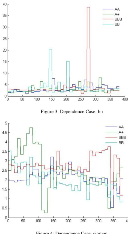
12

Figure 3: Dependence Case: bn

Figure 4: Dependence Case: sigman

Although BB and BBB have a few higher bn in future, they have also high sigman at those

times.

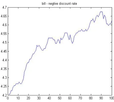
13

Figure 5: An American Treasury Bill’s Daily Return Rate

There’s large number of negative discounted rate appeared.

5. Conclusion and Development

This model is an general case of Philipp J. Schonbucher (20022003) in pricing defaultable

derivative. The parameters of extended Vasicek model are always assume to be constant

functions in the past, we generalize each to be step function. And we provide method to rate the

corporate bond.

And there are still much to be encouraged. An shortcoming is the intensity model: COX

process is nonnegative, this says that when corporate default, it can’t redeem the false. But we

couldn’t know defaultable bond default besides maturity and the days who pays interest rate to us,

so they must have chance to redeem such defaults.

In this paper, we use the fractional recovery model. But, does it suitable? Some may find more

suitable methods.

Although many people think about interest rate must be nonnegative, so they choose CIR to

replace Vasicek. But we use here is the discounted rate of each bond, there exists many negative

discounted rate, so we choose Vasicek model is also reasonable. And we should improve it more

hardly in the future.

14

References

[1] O. Vasicek, ”An Equilibrim Characterization of the Term Structure,” Journal of Financial Economics, Vol.5 (1997), 177188.

[2] F. Jamshidian, ”An Exact Bond Option Formula,” The Journal of Finance, Vol.44 No.1 (Mar.,1989), 205209.

[3] J. Hull; A. White, ”Pricing InterestRateDerivative Securities,” The Review of Financial Studies, Vol.3 No.4 (1990), 573592.

[4] Cox,J. C.,J. E. Ingersoll, and S. A. Ross, ”A Theory of the Term Structure of Interest Rates,” Econometrica, Vol.53 No.2 (Mar.,1985), 385408.

[5] Rudi Zagst, ”InterestRate Management.”

[6] J. Hull; A. White, ”The General HulWhite Model and Super Calibrationn.” (Aug.,2000)

[7] Philipp J. Schonbucher, ”Tree Implementation of Credit Spread Model for Credit Derivatives”, Journal of Computation (2001) 138

[8] MingChi Chang, YuanChung Sheu, ”Approximate to Derivative Price in the Generalized Vasicek Model,” NCTU Applied Math. Department Working Paper, (May.,2006)