在一維度上的有界形和分割及單一形均分割問題

全文

(1)國立交通大學應用數學系博士論文在一維度上的有界形和分割及單一形均分割問題 The Bounded-shape Sum-partition and the Single-shape Mean-partition Problems in One-dimension 研究生 : 張飛黃指導教授: 黃光明教授. 中華民國九十四年六月.

(2) 在一維度上的有界形和分割及單一形均分割問題 The Bounded-shape Sum-partition and the Single-shape Mean-partition Problems in One-dimension 研究生 : 張飛黃 Student: Fei-huang Chang 指導教授: 黃光明教授 Advisor: Frank K. Hwang 國立交通大學應用數學系博士論文. A Dissertation Submitted to Department of Applied Mathematics College of Science National Chiao Tung University in Partial Fulfillment of the Requirements for the Degree of Doctor of Philosophy in Applied Mathematics June 2005 Hsinchu, Taiwan, Republic of China 中華民國九十四年六月.

(3) Abstract The optimal partition problem considers the partition of n objects into p nonempty parts, and finding a partition(optimal partition) to maximize the objective function F : Rp → R. A brute force method is to compare the values of objective function F (π) for each partition π. Thus, we are concerned with the number of all partitions which determines whether the brute force method is practical. However, a more desirable solution is to prove that the objective function has some suitable property which leads to the existence of an optimal partition in a special class of partitions. Then, we need pay attention only to this class of partitions. The vector of the size of each part is called a shape. If a partition problem has a restriction where the size of each part lies in an interval, then it is called a bounded-shape partition problem. If each interval is degenerated, then it is called single-shape partition problem. In Chapter 2, we use the generating function to count the number of ordered(unordered) shapes and the number of bounded-shape partitions. In Chapter 3, we prove that for bounded-shape sum-partition problem with Schur-convex objective function, there must be a nonmajorized shape such that the corresponding size-consecutive partition is optimal. We also bound the number of nonmajorized shapes, and develop an algorithm to find all nonmajorized shape-types. In Chapter 4, we prove that for single-shape mean-partition problem with quasi-convex objective function, there must be a consecutive optimal partition. We also give some new results for the mean-partition problems.. iii.

(4) 摘要最優分法問題主要是對於目標函數F : Rp → R考慮n個物件分成p個非空部份, 如何找到一個分法π(最優分法), 使得F (π)為最大值。一個最直接的方法是去比較所有分法的目標函數值。此時, 我們關心所有分法的數量, 因為它決定了直接法是否可行。更好的是當目標函數具備有某些性質, 使得某些特定的分法類中含有一最優分法, 我們就可以只關心這一些數量較小的特定分法。每個部分容量所形成的向量我們稱為形, 若一個問題對每個部分的容量分別落於一個區間內, 我們稱為有限形分割問題。若每個區間為單一的點, 則我們稱為單一形分割問題。在第二章, 我們使用生成函數去計算對於有序及無序的有界形分割各有多少形及分法。在第三章, 我們証明對於有界形和分割問題, 當目標函數為 Schur 凸函數, 必存在一不被偏形其所對應的容量連續分法為最優分法。並給出了不被偏形的數量上界及發展了找出所有不被偏等價形的演算法。在第四章, 我們証明對於單一形均分割問題, 當目標函數為準凸函數, 其最優分法必是一連續分法。並且對均分割問題給了一些新的結果。. iv.

(5) 誌謝二十幾年的就學生涯到此算是告一段落了, 今日的我能夠以理工博士的身份結束個人的求學生涯, 要感謝的人實在太多太多, 第一: 要感謝的是在我求學期間指導過我的老師, 首先是當我就讀東華應數系三年級時, 遠從清大來花蓮任教一年的張企老師, 您給了我大學生涯中最有意義的一個A+ , 這個全班唯一的一個A+ , 讓我重新開始拾起書本, 也讓我了解問一個好問題是多麼的有價值, 沒有您就沒有今日的我。再來是我碩士班的指導教授王立中老師以及在我就讀大學及碩士期間給我很多生涯規劃上建議的郭大衛老師, 是因為這二位老師對學生我的指導及愛護, 使我能在碩士期間得以有論文發表, 也種下了來交大就讀博士班的種子。而來到交大後, 感謝系上的黃大原老師、傅恆霖老師以及翁志文老師, 教導了我許多組合學上的基本知識; 也謝謝陳秋媛老師給予我很多課業及生活上的意見, 最後也是最重要的要感謝我博士班的指導老師, 黃光明老師, 是您做學問及做人做事的態度深深影響著我, 不但能夠給予我課業上的解惑, 也能在我偷懶或做錯事時給我當頭棒喝, 還能忍受我天馬行空的想法以及耐心的指導我許許多多的缺點; 當學生的我只要有一點點表現, 就給予很大的讚賞及鼓勵, 而當表現不好時, 就馬上給予告誡, 但於他人前仍是稱許學生的好, 對於您的身教及言教, 做學生的我現在無以為謝, 只有將來於研究這條路上盡心盡力, 方是最好的回報。第二: 還要感謝我許許多多的好朋友, 首先是陪我一同走過十幾個年頭的國小、國中同窗及好友, 欽垚、世芳、奕霖、麒銘、志銘, 有你們在身旁的日子裡總是特別歡樂, 總會在不經意時想起一同騎機車上草山的日子, 總是在半夜蹺家打撞球, 還有兩個瘋子半夜騎機車到花蓮來找我還是當天來回, 讓我在情緒煩燥的同時或隨時, 有人可以陪我一起瘋狂, v.

(6) 一起打球, 一起做一些很無聊的事, 但這卻是我一直往前走的動力之一, 也一直是我很珍惜的回憶。高中同學, 翊帆、明謙, 雖是不常見面, 但是一見面卻又熟得跟天天見面似的, 能認識你們是我的福氣; 大學好友及碩士同學, 鴻志、于菁、俊良, 總是可以常常一聊就聊得沒日沒夜的朋友; 最後感謝交大碩班91及92級組合組的學弟妹 (族繁不及備載), 同學君逸、宏賓以及學姐琲琪, 謝謝你們在交大期間的陪伴、照顧及帶給我一個歡樂的交大生活。第三: 就是謝謝我的家人, 爸、媽及老弟是你們在背後的支持, 我才能無憂無慮的完成我的學業, 當然也要謝謝我的岳父及岳母, 能夠體諒我的難處, 肯將您們心愛的女兒托付給我, 也在我求學的最後一段時間能幫我照顧小孩, 當然最要感謝的是一直支持我的親愛老婆蕙慈, 從大學時期起, 就一直陪伴在我的身旁, 很多時候都是有你的鼓勵與支持, 才能讓我這一路走的這樣順利, 最後也謝謝最新產生的動力及希望, ”騰達”, 看著你小小的身軀, 老爸就會覺得一切的努力都是值得的。誌謝文短, 感謝卻意長, 謹以此篇論文, 獻給您們。 (p.s.要感謝的人實在太多太多, 總之謝謝曾經或者一路陪我走來的師長、朋友及家人們). vi.

(7) Contents Abstract. iii. 中文摘要. iv. 誌謝. v. Contents. vii. 1 Introduction 1.1 The one dimensional partition problem . . . . . . . . 1.2 The bounded-shape sum-partition problem for Schur objective function . . . . . . . . . . . . . . . . . . . . 1.3 The polytope approach to the sum-partition problem 1.4 The mean-partition problem . . . . . . . . . . . . . .. . . . . convex . . . . . . . . . . . .. .. 1 1. . . .. 3 5 6. 2 Counting the Number of Bounded-shape 7 2.1 The generating function approach . . . . . . . . . . . . . . . . 7 2.2 A neat solution . . . . . . . . . . . . . . . . . . . . . . . . . . 10 3 The 3.1 3.2 3.3 3.4. Sum-partition Problem Nonmajorized shapes . . . . . . . . . . . . . . . . . . The number of nonmajorized shape-types . . . . . . . Identifying all nonmajorized shapes and shape-types . Determining the existence of a majorizing shape . . .. vii. . . . .. . . . .. . . . .. . . . .. . . . .. 12 13 18 21 32.

(8) 4 The Mean-partition Problem 35 4.1 Linear transformation of mean-partition problems to sum-partition problems . . . . . . . . . . . . . . . . . . . . . . . . . . . . . . 36 4.2 Supermodularity of λM . . . . . . . . . . . . . . . . . . . . . . 38 4.3 Some new results in the mean-partition problem . . . . . . . . 42 5 Conclusion and remarks. 45. Reference. 47. viii.

(9) Chapter 1 Introduction In this Chapter, we introduce the background of the optimal partition problem and give a summary of the following Chapters.. 1.1. The one dimensional partition problem. The partition problem studies the partitioning of n numbers into finite nonempty parts so as to maximize an objective function subject to certain constraints on the number of elements in each part. Applications of the partition problem include inventory grouping, scheduling, reliability, graph partitioning, hypothesis testing in statistics, circuit layout, clustering, symbolic computation, location problems, storage allocation, group testing, system reliability, etc.., see [16] for a survey. Consider a partition π of {1, ..., n} into p nonempty parts π1 , ..., πp . If the number of parts is fixed to be p, we call it a p-partition(size-partition); otherwise we call it an open partition. Let n1 , ..., np be the sizes of π1 , ..., πp where p P ni = n. We define the shape of π as the vector (n1 , ..., np ). If the cardii=1. nalities of the p parts are fixed to be (n1 , ..., np ), then we call it a (n1 , ..., np )partition(single-shape-partition). If the size of each parts must lie in a range, i.e., nonnegative integer p-vectors L = (L1 , ..., Lp ) and U = (U1 , ..., Up ) are. 1.

(10) given where. p X. Li ≤ n ≤. i=1. p X. Ui ,. (1.1.1). i=1. and the shape (n1 , ..., np ) of a feasible partition satisfies for each i Li ≤ ni ≤ Ui , i ∈ {1, ..., p},. (1.1.2). then we call it a bounded-shape-partition. Define Γ(L, U ) to be the set of all partitions whose shapes satisfy (1.1.1) and (1.1.2). If the number of parts is fixed at p and only a set of shapes is allowed, then we called it a constrained-shape-partition. In addition, we have the two categories of ordered partitions and unordered partitions. An ordered partition is a sequence (π1 , ..., πp ), while an unordered partition is a set {π1 , ..., πp }. Given an objective function F (π), our goal is to find a partition(optimal solution) to maximize it. A brute-force way is to enumerate and evaluate all legitimate partitions to get the optimal solution of the objective function. Whether this is a practical method depend on the number of legitimate partitions. The counting of ordered and unordered partitions for open partitions, size partitions and shape partitions are fundamental combinatorial problems and have been well documented [16]. Although, theoretically, we could count bounded-shape partitions also by summing up all legitimate shapes, that could be unwieldy in practice. We will study the generating function approach to count bounded-shape partitions in Chapter 2. Suppose we know that the objective function has an optimal solution in a special class of partitions, then we need pay attention only to this class of partitions. Two such classes are consecutive partitions and size-consecutive partitions. A partition is called consecutive if each part consists of consecutive integers. A consecutive partition is called size-consecutive(reverse-sizeconsecutive) if ni > nj implies that every member in πi is larger (smaller) than every member in πj . Of course, given any integer vector (n1 , . . . , np ) p P which satisfies ni = n, there exist a size-consecutive and a reverse-sizei=1. consecutive partition with shape (n1 , . . . , np ); in fact, they are unique when2.

(11) ever the ni ’s and the θi ’s are distinct. In Chapter 3, we prove that when the objective function of the sum-partition problem with bounded-shape is Schur convex(see Sec.1.2), we need pay attention only to size-consecutive partitions with nonmajorized shapes. In Chapter 4, we show that for the single-shape partition, results obtained for the sum-partition problem also apply to the mean-partition problems.. 1.2. The bounded-shape sum-partition problem for Schur convex objective function. For a vector a = (a1 , ..., ap ) in Rp , let a[i] be the i-th largest member of {a1 , . . . , ap }. Given vectors a and b in Rp , we say that a majorizes b if k X i=1. a[i] ≥. k X. b[i] for k = 1, . . . , p − 1. (1.2.1). i=1. and. p X. ai =. i=1. p X. bi .. (1.2.2). i=1. We say that a strictly majorizes b if a ∈ S majorizes b but b does not majorize a. If a majorizes b for each b ∈ S ⊆ Rp , then a is called majorizing vector in S, if a is not majorized by any b ∈ S, a is called a nonmajorized vector in S. A real-valued function f on Rp is Schur convex if f (a) ≥ f (b) whenever a majorizes b. A Schur convex function is known to be symmetric. For a partition π = (π1 , ..., πp ) let θπ = (. X. θj , . . . ,. j∈π1. X. θj ),. (1.2.3). j∈πp. Hwang and Rothblum [15] considered the sum-partition problem of maximizing the objective function F (π) = f (. X. j∈π1. θj ,. X j∈π2. 3. θj , . . . ,. X j∈πp. θj ),. (1.2.4).

(12) over partitions π having shape in a prescribed set with f being Schur convex. In particular, they proved Theorem 1.2.1. Theorem 1.2.1. Suppose f is Schur convex, Γ is a set of positive integer p-vector that sum to n and π is a partition with shape in Γ which is majorized by a shape (n1 , . . . , np ) ∈ Γ. (a) If θi ≥ 0 for i = 1, . . . , n, then every size-consecutive partition π 0 with shape (n1 , . . . , np ) has f (θπ0 ) ≥ f (θπ ). (b) If θi ≤ 0 for i = 1, . . . , n, then every reverse-size-consecutive partition π 0 with shape (n1 , . . . , np ) has f (θπ0 ) ≥ f (θπ ). In particular, when Γ contains a single shape, if n1 ≤ ... ≤ np , then the following explicit partitions are optimal under (a) or (b), respectively πi = (. i−1 X. nj + 1, ...,. i X. j=1. and πi = (n −. i X j=1. nj ) for i = 1, ..., p. (1.2.5). j=1. nj + 1, ..., n −. i−1 X. nj ) for i = 1, ..., p.. (1.2.6). j=1. They also considered the problem with bounded shapes. They gave the example where n = 9, p = 3, L = (1, 2, 2) and U = (5, 4, 4) to show that a majorizing shape may not exist. They also gave a sufficient condition for the existence of the majorizing shape. The sufficient condition is that the order of upper bounds over the p parts equal to the order of lower bounds. By Theorem 1.2.1, if f is Schur convex and Γ = Γ(L, U ) has the majorized shape, then we can find an optimal solution in the (reverse)size-consecutive class. In Chapter 3, we extend Theorem 1.2.1 to the case when the majorized shape doesn’t exist and Γ is a set of bounded-shapes.. 4.

(13) 1.3. The polytope approach to the sum-partition problem. Given a real-value function λ on the subsets of {1, ..., p} with λ(φ) = 0, each permutation σ = (σ1 , ..., σp ) of {1, ..., p} defines a vector λσ = ((λσ )1 , ..., (λσ )p ) such that S S (λσ )k = λ( ji=1 σi ) − λ( j−1 i=1 σi ), with σj = k for 1 6 k 6 p. λ is called supermodular if for all subsets I, J of {1, ..., p}, λ(I ∪ J) + λ(I ∩ J) > λ(I) + λ(J), and strictly supermodular if the inequality is strict for all I, J not satisfying I ⊆ J or J ⊆ I. The permutation polytope induced by λ, denoted H λ , is the convex hull of {λσ : all σ}. For example, Shapley [18] studied the case of convex p-person game. For a subset I ⊆ {1, ..., p}, let λ(I) denote the payoff to I, if the members of I form an alliance. Then stability of an alliance I ∪ J requires λ to be supermodular. The core of a convex p-person game is the solution set of the linear inequality system X. xi ≥ λ(I) for all I ⊆ {1, ..., p} and. p X. xi = λ({1, ..., p}).. (1.3.1). i=1. i∈I. Let C λ denoted the polytope defined by (1.3.1). Shapley [18] proved Theorem 1.3.1. Suppose λ is supermodular. Then (a) H λ = C λ , (b) the vectices of H λ are precisely the λσ ’s where σ ranges over all permutations of {1, ..., p}. Gao et al.[9] studied the single-shape sum-partition problem to maximize P P an objective function f ( θj , ..., θj ). For I a subset of {1, ..., p}, define j∈π1 j∈πp P n(I) = ni . They defined i∈I. λS (I) =. n(I) X j=1. 5. θj. (1.3.2).

(14) and proved λS is supermodular. Here, H λS is the convex hull of all partitions corresponding to {(λS )σ : all σ} (each partition is a point), and C λS is the polytope defined by n PP P θj > λS (I) for all I ⊆ {1, ..., p} and θj = λS ({1, ..., p}). i∈I j∈πi. j=1. Let P denote the convex hull of all partitions satisfying the given single shape. Clearly, H λS ⊆ P ⊆ C λS . By Theorem 1.3.1, H λS = P = C λS . They proved the existence of a consecutive optimal partition for the single-shape partition problem when f is quasi-convex.. 1.4. The mean-partition problem. Consider N = {1, ..., n} where each element i in N is associated with a number θi ∈ R. Partition problems are further classified by their objective function F (.). For a subset S of {1, ..., n}, let 1 X θi ∈ R, (1.4.1) θ¯S = |S| i∈S and for a partition π = (π1 , ..., πp ), let θ¯π = (θ¯π1 , ..., θ¯πp ) ∈ Rp .. (1.4.2). A class of partition is the mean-partition problem in R in which F (π) = g(θ¯π ),. (1.4.3). where g is a real-valued function on Rp . The mean-partition polytope corresponding to a set of partitions Π is denoted by M Π . While the sum partition problem has been dominating in optimal partition problems, the mean partition problems have also been considered. Anily and Federgruen [1] first studied the single-shape mean-partition problem. In Chapter 4, we will give an approach to solve the single-shape mean-partition problem, and discuss the difficulties of the bounded-shape mean-partition problem. Finally, we give some new results in the mean-partition problem. 6.

(15) Chapter 2 Counting the Number of Bounded-shape In this chapter, we use the generating function approach to count boundedshape partitions. When the θi ’s are constant, then the number of boundedshape partitions is reduced to the number of bounded shapes. We obtain a neat solution of that number for ordered partitions.. 2.1. The generating function approach. For given lower bound Li and upper bounds Ui , 1 ≤ i ≤ p, define #∗n : The number of ordered bounded shapes. ∗. #n : The number of unordered bounded shapes. #n : The number of ordered bounded-shape partitions. #n : The number of unordered bounded-shape partitions. Define ∗. L =. p X i=1. 7. Li.

(16) and gn (x) =. p Y. Ã. i=1. ≡. X. Ui X. ! aj xj. j=Li. c k xk .. k≥L∗. It is well known [2] that (k). ck =. gn (0) . k!. ∗. We show that #∗n , #n , #n and #n can be expressed as different functions of cn . Theorem 2.1.1. (i) #∗n = cn by setting aj = 1 in gn (x). ∗. (ii) #n = the number of distinct terms in cn . (iii) #n = n!cn by setting aj = 1/(j!). (iv) #n = same as (iii) except counting only distinct terms in cn , and diQ Q viding a term pi=1 aei i by pi=1 (ei !). Proof. (i) Every ordered shape (n1 , n2 , . . . , np ) summing to n contributes 1 to cn . (ii) Two shapes (n1 , . . . , np ) and (n01 , . . . , n0p ) are not distinguishable if {n1 , . . . , np } = {n01 , . . . , n0p }. A shape (n1 , . . . , np ) is preserved in the coefficient term an1 , . . . , anp . Hence we count only distinct an1 , . . . , anp (as coefficient, the ordering is not important) terms. ¡ n ¢ (iii) Each shape (n1 , . . . , np ) yields n1 ,...,n distinct partitions. p (iv) The division is because interchanging two parts of same size results in the same unordered partition. 8.

(17) Example 1. n = 10, n1 ∈ [2, 4], n2 ∈ [2, 6], n3 ∈ [3, 5]. (i) g(x) = (x2 + x3 + x4 )(x2 + x3 + x4 + x5 + x6 )(x3 + x4 + x5 ) = x7 + 3x8 + 6x9 + 8x10 + 9x11 + 8x12 + 6x13 + 3x14 + x15 . There are c10 = 8 ordered bounded shapes which are (2, 3, 5), (2, 4, 4), (2, 5, 3), (3, 2, 5), (3, 3, 4), (3, 4, 3), (4, 2, 4), (4, 3, 3). (ii) g(x) = (a2 x2 + a3 x3 + a4 x4 )(a2 x2 + · · · + a6 x6 )(a3 x3 + a4 x4 + a5 x5 ) = · · · + (3a2 a3 a5 + 2a2 a24 + 3a23 a4 )x10 + . . . . Hence, there are 3 unordered bounded shapes which are (2, 3, 5), (2, 4, 4), (3, 3, 4). (iii) x2 x3 x4 x2 x6 x3 x4 x5 + + )( + · · · + )( + + ) 2! 3! 4! 2! 6! 3! 4! 5! 1 7 11 8 89 9 7 10 17 11 = x + x + x + x + x + .... 24 288 4320 960 8640 7 Hence, there are 10! × 960 = 26460 ordered bounded-shape partitions. g(x) = (. (iv) a2 x2 a4 x4 a2 x2 a 6 x6 a 3 x3 a5 x5 + ··· + )( + ··· + )( + ··· + ) 2! 4! 2! 6! 3! 5! 3a2 a3 a5 2a2 a24 3a23 a4 10 = ··· + ( + + )x + . . . . 1440 1152 864 The number of unordered bounded-shape partitions is 1 10! 1 10! 1 10! × + × + × = 6195. 1440 (1!)(1!)(1!) 1152 (1!)(2!) 864 (2!)(1!) g(x) = (. Although a generating function counting is equivalent to enumeration, it gives a particular way of enumeration, hence doable by a computer program. 9.

(18) 2.2. A neat solution. We show that the generating function approach leads to a neat formula for the number of ordered bounded shapes. Define Ri = Ui − Li , 1 ≤ i ≤ p, p X S = {(s1 , . . . , sp ) | si ∈ {0, Ri + 1} for 1 ≤ i ≤ p, si ≤ n − L∗ } i=1. and ∗. sp+1 = n − L −. p X. si .. i=1. Let |(s1 , . . . , sp )| denote the number of positive si . Theorem 2.2.1.. µ. X. #n =. (−1). |(s1 ,...,sp )|. (s1 ,...,sp )∈S. ¶ p + sp+1 − 1 . p−1. Proof. g(x) = (xL1 + xL1 +1 + · · · + xU1 ) . . . (xLp + xLp +1 + · · · + xUp ) ∗. = xL (1 + x + · · · + xR1 )(1 + x + · · · + xR2 ) . . . (1 + x + · · · + xRp ) ∗. = xL (1 − xR1 +1 )(1 − xR2 +1 ) . . . (1 − xRp +1 )(1 − x)−p . Using the Leibniz formula, Ãm !(n) Y fi (x) =. µ. X n1 +···+nm =n. i=1. ¶Y m n (n ) fi i (x), n1 , . . . , nm i=1. where ni is the largest exponent of fi (x), on the first p + 1 terms of g(x), ¶ · sp+1 ¸ X µ d n (n) |(s1 ,...,sp )| ∗ −p g (0) = (−1) L !s1 ! . . . sp ! (1 − x) L∗ , s1 , . . . , sp , sp+1 dxsp+1 x=0 (s1 ,...,sp )∈S. X. ¤ (p + sp+1 − 1)! £ (1 − x)−p−sp+1 x=0 sp+1 ! (p − 1)! (s1 ,...,sp )∈S µ ¶ X £ ¤ |(s1 ,...,sp )| p + sp+1 − 1 = n! (−1) (1 − x)−p−sp+1 x=0 . p−1. =. n!. (−1)|(s1 ,...,sp )|. (s1 ,...,sp )∈S. 10.

(19) (n). gn (0) Thus #n = cn = = n!. X. µ |(s1 ,...,sp )|. (−1). (s1 ,...,sp )∈S. ¶ p + sp+1 − 1 . p−1. A size-partition can be interpreted as a bounded-shape partition with uniform bounds Li = 1, Ui = n. Then L∗ = p, Ri = n − 1, 1 ≤ i ≤ p. Necessarily, si = 0 for 1 ≤ i ≤ p. and sp+1 = n − L∗ = n − p. Corollary 2.2.2. The number of ordered size-partitions is. ¡n−1¢ p−1. .. Example 2. n = 14, n1 ∈ [2, 4], n2 ∈ [2, 8], n3 ∈ [3, 6]. R1 = 2, R2 = 6, R3 = 3, L∗ = 7, n − L∗ = 7. S = {(0, 0, 0), (3, 0, 0), (0, 7, 0), (0, 0, 4), (3, 0, 4)}. Hence ¡ ¢ ¡ ¢ ¡ ¢ #([2, 4], [2, 8], [3, 6]) = (−1)0 3+7−1 + (−1)1 3+4−1 + (−1)1 3+0−1 3−1 3−1 3−1 ¡ ¢ ¡ ¢ 2 3+0−1 + (−1)1 3+3−1 + (−1) 3−1 3−1 ¡9¢ ¡6¢ ¡5¢ = 2 − 2 −1− 2 +1 = 11. The shapes are: (2, 6, 6), (2, 7, 5), (2, 8, 4), (3, 5, 6), (3, 6, 5), (3, 7, 4), (3, 8, 3), (4, 4, 6), (4, 5, 5), (4, 6, 4), (4, 7, 3). 11.

(20) Chapter 3 The Bounded-shape Sum-partition Problem in R1 with Schur Convex Objective Function In this chapter, we consider the bounded-shape sum-partition problem in R1 with Schur convex objective function. We will show that the θi ’s are one-sided, one can restrict attention to (reverse) size-consecutive partitions with a nonmajorized shape. As a (reverse) size-consecutive partition with a given shape is easy to determine(see (1.2.5) and (1.2.6)), the problem of finding an optimal partition is reduced to the task of identifying a set of shapes that contains all nonmajorized ones. Since Schur convex functions are symmetric, they do not differentiate between partitions that are obtained by part-permutations as long as the corresponding coordinate-permutations of the shapes are feasible. Thus, we may restrict attention to representatives of shape-types which are the equivalence classes of shapes with respect to coordinate-permutations. We will study nonmajorized shapes, bound their numbers and develop algorithms to enumerate them, too. Our study extends the analysis of a previous paper [15] which discussed the above problem assuming the existence of a majorizing shape.. 12.

(21) 3.1. Nonmajorized shapes. We explore the relation between shape-majorization and the optimization problem with Schur-convex objective function over partitions introduced in the Introduction. In particular, we explore the role of nonmajorized shapes, with respect to Γ(L, U ). Corollary 3.1.1. Suppose f and Γ are as in Theorem 1.2.1, but no majorizing shape exists. (a) If θi ≥ 0 for i = 1, . . . , n, then there is a nonmajorized shape in Γ such that any corresponding size-consecutive partition is optimal. (b) If θi ≤ 0 for i = 1, . . . , n, then there is a nonmajorized shape in Γ such that any corresponding reverse-size-consecutive partition is optimal. Corollary 3.1.1 implies that when f is Schur convex and the θi ’s are one-sided, it suffices to restrict attention to (reverse) size-consecutive partitions whose shapes are nonmajorized. Of course, the symmetry of Schur convex functions implies that all size-consecutive partitions with the same shape have the same objective value F (as determined by (1.2.4)). We conclude that the underlying optimization problem can be solved by obtaining a list that contains all nonmajorized shapes, determining corresponding sizeconsecutive partitions, and evaluating the right-hand side of (1.2.4) for each one of them to select the best. Further, it suffices to consider only representatives of all nonmajorized shape-types. The remainder of our paper will focus on studying and identifying nonmajorized shapes and shape-types with respect to sets of the form Γ(L, U ). In the bounded-shape case which the majoring shape doesn’t exist [4], consider a vector a ∈ IRp and J ⊆ {1, . . . , p}, let aJ denote the subvector of a consisting of the coordinates indexed by J. Lemma 3.1.2. Consider vectors a and b in IRp with. p P i=1. ai =. p P. bi and a set. i=1. J ⊆ {1, . . . , p} for which ai = bi for each i ∈ {1, . . . , p} \ J. Then [aJ majorizes bJ ] ⇔ [a majorizes b]; 13. (3.1.1).

(22) further (3.1.1) holds with “majorizes” replaced by “strictly majorizes”. Proof. Suppose aJ majorizes bJ . Let k ∈ {1, . . . , p−1} be given and let K be k P P a subset of {1, . . . , p} with b[i] = bi . Set m ≡ |K ∩ J|. As aJ majorizes m P. bJ we have that. i=1 m P. (aJ )[i] ≥. i=1. i∈K. P. (bJ )[i] ≥. i=1. for each i ∈ {1, . . . , p} \ J implies that k X. m X. a[i] ≥. i=1. ai. i∈K∩J c. i=1. X. ≥. X. (aJ )[i] +. bi , hence, the assertion ai = bi. i∈K∩J. bi +. X. bi =. X. i=K∩J c. i∈K∩J. bi =. k X. b[i] .. i=1. i∈K. P As k ∈ {1, . . . , p − 1} was selected arbitrarily and (by assumption) pi=1 ai = Pp i=1 bi , we conclude that a majorizes b. Next, assume that a majorizes b. As ai = bi for each i ∈ {1, . . . , p} \ J p p P P P P and ai = bi , we have that ai = bi . Next, let k ∈ {1, . . . , |J| − 1} i=1. i=1. i∈J. i∈J. P. be given and let K be a subset of J with. ai =. k P. (aJ )[i] . Consider the set. i=1. i∈K. W consisting of all indices i ∈ {1, . . . , p} \ J for which ai ≥ min{ai : i ∈ K}, and let m ≡ |W | (W = φ and m = φ is possible). For k 0 = k + m, we have k0 P P P a[i] = ai + ai . Consider any set H \ J with |H| = k. As a that i=1. majorizes b,. i∈K. P i∈K. ai +. i∈W. P. ai =. k0 P. a[i] ≥. i=1. i∈W. k0 P. b[i] ≥. i=1. P. bi +. i∈H. P. bi .. i∈W. As ai = bi for each i ∈ {1, . . . , p} \ J ⊇ W , we conclude that k P. (aJ )[i] =. i=1. P. ai ≥. i∈K. P. bi , .. i∈H. The freedom in selecting H and k allows us to conclude that aJ majorizes bJ .. 14.

(23) The strict version of (3.1.1) follows directly from the weak version and the observation that a vector u strictly majorizes another vector v if and only if u majorizes v and v does not majorize u. Lemma 3.1.2 will be used particularly with sets J consisting of two elements. Throughout the remainder of this section, let L and U be nonnegative integer p-vectors that satisfy (1.1.1)–(1.1.2). In particular, we refer to a nonmajorized shape under Γ(L, U ) as a nonmajorized shape. We next explore the properties of such shapes. Lemma 3.1.3. Consider the following properties of a shape s = (n1 , . . . , np ): (a) s is nonmajorized; (b) there exist no distinct i and j such that Lj < ni < Ui and Lj < nj < Ui ,. (3.1.2). (c) if for distinct i and j, Lj < nj and ni < Ui , then ni < nj ; and (d) there exists at most one index i with Li < ni < Ui . Then (a) ⇒ (b) ⇒ (c) ⇒ (d). Proof. (a) ⇒ (b). Suppose ni and nj satisfy (3.1.2) where i 6= j. Without loss of generality, assume that ni ≥ nj . Then s is majorized by the shape obtained from s by increasing ni to max{ni , nj } + 1, and decreasing nj to min{ni , nj } − 1 (see Lemma 3.1.2). (b) ⇒ (c). Suppose condition (b) holds, and i and j are indices satisfying Lj < nj , ni < Ui and i 6= j. By condition (b), either Lj ≥ ni or nj ≥ Ui . In the former case, ni ≤ Lj < nj and in the latter case nj ≥ Ui > ni . (c) ⇒ (d). Suppose condition (c) holds, and i and j are indices satisfying Li < ni < Ui , Lj < nj < Uj and i 6= j. We will establish a contradiction. Indeed, if ni ≥ nj we get a direct violation of (c) and if ni < nj we get a violation of (c) with the roles of i and j reversed. The following examples shows that condition (b) of Lemma 3.1.3 does not imply condition (a). 15.

(24) Example 3. Let U = (5, 5, 5, 2), L = (1, 4, 3, 1), s = (5, 4, 3, 1) and s0 = (2, 5, 5, 1). It is easy to verify that s is majorized by s0 . To see that there exist no i and j satisfying (3.1.2), observe that the only coordinate of s that is strictly larger than the lower bound is the first one, so if (3.1.2) is satisfied necessarily j = 1. But, n1 is not strictly below any upper bound. For a given shape s, call part i an upper part, a middle part or a lower part if, respectively, ni = Ui , Li < ni < Ui , ni = Li . If part i has Li = Ui , each shape (n1 , . . . , np ) ∈ Γ(L, U ) has ni = Li = Ui . Thus, in search of nondominated shapes under (L, U ), one can ignore such parts. Of course, when L ¿ U (i.e., Li < Ui for each i), the parts are classified uniquely. Lemma 3.1.3 shows that a nonmajorized shape can have at most one middle part. Suppose L ¿ U . Given a shape s = (n1 , . . . , np ), let B(s) stand for the p-vector whose elements are the symbols L, M and U constructed in the following way: For a permutation i1 , . . . , ip of the coordinates for which ni1 ≥ ni2 ≥ · · · ≥ nip , let B(s)t for t = 1, . . . , p be L, M, U according to it being an upper, middle or lower part. The next result shows that no ambiguity can arise in the definition of B(s), i.e., it is uniquely defined, and that B(s) has a simple structure. Lemma 3.1.4. Suppose L ¿ U and s = (n1 , . . . , np ) is a nonmajorized shape. Let (i1 , . . . , ip ) be a permutation of (1, . . . , p) such that ni1 ≥ ni2 ≥ · · · ≥ nip . Then: (a) nir = nit for r, t ∈ {1, . . . , p} implies ir and it are either both upper parts or both lower parts. (b) B(s) has the form (U, . . . , U, M, L, . . . , L) or (U, . . . , U, L, . . . , L). Proof. (a) If nir = nit , ir is a lower-part and it is not, then Lit < nit = nir = Lir < Uir , in contradiction to implication (a) ⇒ (b) in Lemma 3.1.3. A similar argument applies to prove that if ir is an upper-part, so is it . (b) The implication (a) ⇒ (c) in Lemma 3.1.3 assures that if nj = Uj > Lj and ni < Ui , then ni < nj , and that if ni = Li < Ui and nj > Lj , then 16.

(25) ni < nj . It follows that for every permutation i1 , . . . , ip of 1, . . . , p with ni1 ≥ · · · ≥ nip and r, t ∈ {1, . . . , p} [nir = Uir and nit < Uit ] ⇒ [r < t] and [nit = Lit and nir > Lir ] ⇒ [r < t]. These implications establish the asserted structure of B(s). We conclude this section with an observation about a necessary difference between two nonmajorized shapes. Lemma 3.1.5. Two distinct nonmajorized shapes s = (n1 , . . . , np ) and s0 = (n01 , . . . , n0p ) must differ in at least two coordinates; further, if such s and s0 differ in exactly two coordinates, say coordinates i and coordinate j, where ni > n0i , then s0 is obtained from s by permuting these coordinates, ni = Ui or nj = Lj. (3.1.3). n0i = Li or n0j = Uj .. (3.1.4). and P P Proof. Suppose shapes s and s0 differ in only one part, then i ni 6= i n0i , contradicting the fact that both are shapes and their coordinate sum is n. Next, assume that s = (n1 , . . . , np ) and s0 = (n01 , . . . , n0p ) are nonmajorized shapes that differ only in coordinates i and j. As neither strictly dominates the other (they are nonmajorized), we have that s0 is obtained from s by permuting two coordinates, say coordinates i and j. Now, suppose ni < n0i = nj . As Lj ≤ nj = n0i < ni ≤ Ui , the implication (a) ⇒ (b) in Lemma 3.1.3 assures that either ni = Ui or nj = Lj , and (applying the result on s0 with the roles of i and j reversed), either n0j = Uj or n0i = Li . We say that two shapes are equivalent if one is obtained from the other by coordinate-permutation. Of course, not all coordinate-permutations of a shape in Γ(L, U ) are necessarily in Γ(L, U ). 17.

(26) Corollary 3.1.6. If s and s0 are nonmajorized shapes which are not equivalent, then they differ in at least 3 coordinates.. 3.2. The number of nonmajorized shape-types. In this section, we continue to assume that L and U are integer p-vectors satisfying (1.1.1) and L ¿ U . As strict-majorization is invariant of the corresponding shape-types, we can and will refer to nonmajorized shapetypes. We note that a single nonmajorized shape-type may correspond to many shapes as example 4. Example 4. Let L = (1, . . . , 1), U = (2, . . . , 2) and p < n < 2p. Then all nonmajorized shapes are equivalent and each such shape, say (n1 , . . . , np ) is determined by a set J of {1, . . . , p} consisting of n − p elements, where ni = 2 if i ∈ J and ni = 1 otherwise. So, there is a single nonmajorized shape-type ¡ p ¢ that corresponds to n−p nonmajorized shapes. A shape-type can be identified with the multiset {n1 , . . . , np } where (n1 , . . . , np ) is a shape in Γ(L, U ). For a nonmajorized shape s = (n1 , . . . , np ), let U (s), M (s) and L(s) be set of corresponding upper-, middle- and lower-parts of s, that is, U (s) = {j ∈ {1, . . . , p} : nj = Uj }, M (s) = {j ∈ {1, . . . , p} : Lj < nj < Uj } and L(s) = {j ∈ {1, . . . , p} : nj = Lj }. Lemma 3.2.1. Suppose s = (n1 , . . . , np ) and s0 = (n01 , . . . , n0p ) are nonmajorized shapes that are not equivalent. Then: (a)U (s) 6= U (s0 ), and (b)if U (s0 ) is included in U (s), then M (s0 ) contains a single element j ∈ / U (s) that satisfies Ui0 > n0j for every i in U (s0 ) (3.2.1) and Ui ≤ n0j for every i in U (s) \ U (s0 ). 18. (3.2.2).

(27) Proof. (a) Lemma 3.1.3 assures that |M (s)| ≤ 1 and |M (s0 )| ≤ 1. Thus, if U (s) = U (s0 ), then s and s0 can differ in at most 2 coordinates; it then follows from Corollary 3.1.6 that s and s0 are equivalent, in contradiction to the assertion that they are not. (b) Suppose U (s) ⊇ U (s0 ). As s0 6= s, there is a coordinate j with n0j > nj . We will show that such a j must be in M (s0 ). Indeed, such j cannot be in U (s0 ) for the assertion U (s) ⊇ U (s0 ) would imply j ∈ U (s) and n0j > nj = Uj ; such j can neither be in L(s0 ) because n0j > nj ≥ Lj . So, j must be in M (s0 ). By Lemma 3.1.3, there can be at most a single part in M (s0 ). Thus, M (s0 ) = {j} and j is the single coordinate for which s0 exceeds s. Now, for i in U (s0 ), n0i = Ui > Li . As n0j < Uj , the (a)⇒(c) part of Lemma 3.1.3 implies that n0j < n0i = Ui , proving (3.1.6). Next, assume that i is in U (s) \ U (s0 ). As s and s0 differ by at least 3 coordinates (Corollary 3.1.6), as j is the single coordinate for which s0 exceeds s and as ni = Ui > n0i , we have that i 6= j 0 and n0j − nj > ni − n0i = Ui − n0i .. (3.2.3). Assume that Ui > n0j and we will establish a contradiction. By summing Ui > n0j and (3.2.3), we get that ni > nj . As i is not in U (s0 ), n0i < Ui . Consider the shape obtained from s0 by increasing n0i to Ui and decreasing n0j to n0j − [Ui − n0i ]. As Ui > n0j , this shape majorizes s0 (recall Lemma 3.1.2). Further, (3.2.3) implies that n0j − [Ui − n0i ] > nj ≥ Lj , assuring that the new shape is in Γ(L, U ). As s0 is assumed to be nonmajorized, we have derived a contradiction which established (3.2.2). Corollary 3.2.2. Suppose s, s0 and s00 are nonmajorized shapes where no pair consists of two equivalent shapes, and suppose U (s0 ) and U (s00 ) are both included in U (s). Then U (s0 ) and U (s00 ) are ordered by set-inclusion. Proof. Let s0 = (n01 , . . . , n0p ) and s00 = (n001 , . . . , n00p ). Part (b) of Lemma 3.2.1 assures that M (s0 ) and M (s00 ) are nonempty. Let M (s0 ) = {i} and 19.

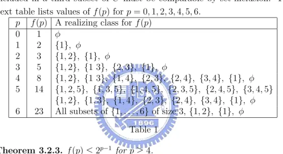
(28) M (s00 ) = {j}. Without loss of generality, assume that n0i ≤ n00j . By Lemma 3.2.1(a), U (s0 ) 6= U (s00 ). Suppose U (s0 ) + U (s00 ). Then there exists k ∈ U (s00 ) ∩ (U (s) \ U (s0 )). By Lemma 3.2.1(b), n0i ≥ Uk > n00j , contradicting our assumption n0i ≤ n00j . We next explore the combinatorial restriction imposed by the conclusion of Corollary 3.2.2. For that purpose, for each integer p ≥ 1, let f (p) be the maximal size of a class C of subsets of {1, . . . , p} which satisfies the conclusions of Corollary 3.2.2, that is, every pair of subsets in C that are included in a third subset of C must be comparable by set-inclusion. The next table lists values of f (p) for p = 0, 1, 2, 3, 4, 5, 6. p f (p) A realizing class for f (p) 0 1 φ 1 2 {1}, φ 2 3 {1, 2}, {1}, φ 3 5 {1, 2}, {1 3}, {2, 3}, {1}, φ 4 8 {1, 2}, {1 3}, {1, 4}, {2, 3}, {2, 4}, {3, 4}, {1}, φ 5 14 {1, 2, 5}, {1, 3, 5}, {1, 4, 5}, {2, 3, 5}, {2, 4, 5}, {3, 4, 5} {1, 2}, {1, 3}, {1, 4}, {2, 3}, {2, 4}, {3, 4}, {1}, φ 6 23 All subsets of {1, . . . , 6} of size 3, {1, 2}, {1}, φ Table 1 Theorem 3.2.3. f (p) ≤ 2p−1 for p ≥ 4. Proof. Consider any p ∈ {1, 2, . . .} and let F (p) realize f (p). Also, let F0 (p) = {U ∈ F (p) : p 6∈ U } and F1 (p) = {U ∈ F (p) : p ∈ U }. As F0 (p) and {U \{p} : U ∈ F1 (p)} are classes of subsets of {1, . . . , p−1} with the property that every pair of sets in class that are included in a third set in the class must be comparable by set-inclusion, we have that |F0 (p)| ≤ f (p − 1) and |F1 (p)| ≤ f (p−1), implying that f (p) = |F (p)| = |F0 (p)|+|F1 (p)| ≤ 2f (p−1). As f (4) = 8 = 23 , we conclude that f (p) ≤ 2p−1 for each p ≥ 4. Corollary 3.2.4. For p ≥ 4, there are at most 2p−1 nonmajorized shapetypes. 20.

(29) Proof. Corollary 3.2.2 and Lemma 3.2.1 show that f (p) bounds the number of nonmajorized shape-types and Theorem 3.2.3 shows that f (p) ≤ 2p−1 . The proof of Corollary 3.2.4 relies on the facts that 2p−1 is an upper bound on f (p) (for p ≥ 4) and that f (p) is an upper bound on the number of unmajorized shape-types. Table 1 demonstrates that 2p−1 is not a tight bound on f (p) and we believe that neither is the second bound. In fact, we conjecture that the number of nonmajorized shape-types can be bounded by ¡ p−1 ¢ , a smaller expression than 2p−1 . (By the Sperner’s lemma [19], ¡b(p−1)/2c ¢ p−1 is the maximum number of independent subsets in the lattice of b(p−1)/2c subsets of {1, . . . , p−1} with set-inclusion as the partial order.) The following examples achieve this (conjectured) bound. Example 5. Let U = (20, 19, 18, 17, 16), L = (1, 2, 3, 4, 5), n = 51. Using the algorithms of Section 4 (see Example 7), one can show that the set of all nonmajorized shape-types contains 6 shapes that are listed below in Table 2. n1 20 20 20 1 1 1. n2 19 2 2 19 19 2. n3 3 18 3 18 3 18. n4 n5 4 5 4 7 17 9 4 9 17 11 17 13. Table 2 Example 6. For any p ≥ 3, let U = (2(p + (d p−1 e)(b p−1 c)) − 1, 2(p + 2 2 p−1 p−1 p−1 p−1 (d 2 e)(b 2 c)) − 2, . . . , p + 2(d 2 e)(b 2 c)), L = (1, 2, . . . , p), and n = p2 + (p − X(p))(d p−1 e)(b p−1 c), where X(p) = 1, if p is odd, otherwise, X(p) = 0. 2 2 Then the number of nonmajorized shape-types achieve conjectured bound.. 3.3. Identifying all nonmajorized shapes and shape-types. Algorithm 1. (For enumerating all nonmajorized shapes in Γ(L, U )) 21.

(30) The input for the algorithm consists of integer p-vectors L and U that satisfy (1.1.1) and L ¿ U . (a) For u = 1, ..., p and A ⊆ {1, ..., p} \ {u} do: P P (i) Set B = {1, . . . , p} \ A \ {u}, UA = i∈A Ui , LB = i∈B Li and Mu = n − UA − LB . (ii) If Lu ≤ Mu ≤ Uu , set Uj for j ∈ A , for j ∈ B , and include (n1 , . . . , np ) in a temporary list that nj = { Lj Mu for j = u , we denote TEMP. (b) Test each shape in TEMP for being nonmajorized by testing if it majorized by any shape in TEMP. The next lemma analyzes Algorithm 1. For the complexity analysis, computational effort counts arithmetic operations and comparisons. Lemma 3.3.1. (a) At the end of step (a), TEMP contains all nonmajorized shapes. (b) The output of Algorithm 1 consists of all nonmajorized shapes in Γ(L, U ). (c) The computational time in executing step (a) of Algorithm 1 is bounded by O(p2p−1 ), and the computational time in executing the complete algorithm is bounded by O(p3 2p ). Proof. (a) Lemma 3.1.3 (part (b)) assures that at the completion of step (a), TEMP contains all nonmajorized shapes. (b) As transitivity of the majorization relation assures that a majorized shape is majorized by some nonmajorized shape, a test for a shape to be nonmajorized is to compare it with all the shapes in TEMP. (c) The number of iterations within step (a) is p2p−1 . The initial calculation of the quantity UA , LB and Mu requires p − 1 addition/subtraction and the updates within each iteration requires O(1) computational time. Hence, the total time to execute step (a) is O(p2p−1 ) and the output may contain up to p2p−1 shapes. 22.

(31) In step (b), each output shape of step (a) is tested against all others. The test requires determining the order statistics of the shapes, creating their partial sums, and executing p comparisons for each pair of shapes. The total time is then bounded by O[(p + p lg p)p2p−1 + (p2p−1 )2 p] = O[p3 22p ]. Given integer p-vectors L and U satisfying (1.1.1)–(1.1.2), the set of floating indices of (L, U ) is defined as {i = 1, . . . , p : Li < Ui }. Also, if G is the set P P of indices of (L, U ) which are not floating, we refer to n − Li (= n − Ui ) i∈G. i∈G. as the availability under (L, U ). We say that the upper bound of index i is effective for (L, U ) if X Ui + Lj ≤ n; (3.3.1) j6=i. when the upper bound of index i is not effective, we refer to the replacement P of Ui by n − Lj ≥ Li as the adjustment of the upper bound of i. Similarly, j6=i. we say that the lower bound of index i is effective for (L, U ) if X Uj ≥ n, Li +. (3.3.2). j6=i. and if the lower bound of index i is not effective, we refer to the replacement of P Li by n − j6=i Uj ≤ Ui as the adjustment of the upper bound of i. Evidently, (1.2.6) and (1.1.1) stay in effect when an upper bound or a lower bound is adjusted. Lemma 3.3.2. Consecutive adjustment of bounds results in a pair of vectors for which all bounds are effective, and this outcome is independent of the order in which bounds are adjusted. Proof. Trivially, consecutive adjustment of bounds must terminate with a pair of vectors for which all bounds are effective. Evidently, (1.2.6) and (1.1.1) stay in effect when a bound is adjusted. Further, if the upper bound of i needs adjustment, all the lower bounds of indices j 6= i are effective throughout any sequence of adjustments; this is the. 23.

(32) case because a decrease of an upper bound does not invalidate the effectiveness of a lower bound and an increase of a lower bound does not invalidate effectiveness of an upper bound. We conclude that if an upper/lower bound of i is adjusted, no lower/upper bound of another j 6= i will require adjustment. Further, the order of consecutive adjustment of upper bounds or of lower bounds has no effect on the outcome. The only remaining case is the adjustment of the upper bound and the lower bound of a particular i—it is easy to verify that here, too, the order of executing these adjustments does not influence the outcome. We refer to the operation that is described in Lemma 3.3.2 as an adjustment of the bounds. We observe that (1.2.6) assures that the bounds of indices that are not floating, are always effective and will therefore not be affected by an adjustment of the bounds. But, bound-adjusting can reduce the set of floating indices. Algorithm 2. (For enumerating all nonmajorized shape-types in Γ(L, U )) The input for the algorithm consists of integer p-vectors L and U that satisfy (1.2.6). Set r = 1. Iteration r: (a) Adjust the bounds (L, U ). Let F and v be the set of floating indices and the availability with respect to the adjusted bounds and set ni = Li = Ui for each i ∈ {1, . . . , p} \ F . If F = ∅, set r = p and go to step (c). Otherwise, set α ≡ maxk∈F Uk and β ≡ mink∈F Lk . (b) Execute, in parallel and record separately the outcome of the following three steps: (i) Select i as any index that maximizes the lower bound among those whose upper bound is α. Set ni ← Ui and Li ← Ui . (ii) Select i as any index that minimizes the upper bound among those whose lower bound is β. Set ni ← Li and Ui ← Li . 24.

(33) (iii) This option is executed only if one identifies an index i that satisfies Ui = α > Uj for each j 6= i, Li = β < Lj for each j 6= i and F \ {i} can be partitioned into two sets A and B such that |A| ≥ 2, |B| ≥ 2 X X max Uk ≤ n − Uj − Lk ≤ min Lj k∈B. j∈A. and Li < n −. X. k∈B. Uj −. j∈A. X. j∈A. L k < Ui .. (3.3.3) (3.3.4). (3.3.5). k∈B. When the above holds with 3.3.4 in strict inequalities, do for each such pair A, B the following: Set nt ← Ut and Lt ← Ut for t ∈ A, ns ← Ls and P P Us ← Ls for s ∈ B, and ni ← µ ≡ n − j∈A Uj − k∈B Lk , Ui ← µ and Li ← µ. Let ni denote the middle part of 3.3.4. Suppose ni = max Uk ≡ Ux . Check k∈B. the existence of a part y in B \ {x} such that |(Lx , Ux ) ∩ (Ly , Uy )| ≥ 2. If no such y exists, then output this shape-type as in the 3.3.4 in strict inequalities case. Similarly, suppose ni = min Lj = Lz . Check the existence of a part w in j∈A. A \ {z} such that |(Lz , Uz ) ∩ (Lw , Uw )| ≥ 2. If no such w exists, then output this shape-type. (c) If r = p, output the shape-types of all generated shapes in step (b)(i) and (b)(ii). Otherwise, replace r with r + 1 and go to step (a) with each outcome of step (b)(i) and of step (b)(ii). Remarks. (1)Step (b) of Algorithm 2 allows a selection between 3 options. Option (iii) can be executed only if one identifies an index i with Ui > Uj and Li < Lj for each j 6= i. When such an index i is identified, options (i) and (ii) will be executed with this particular selection of i. Option (iii) will then be followed for each partition of F \ {i} into sets A and B that satisfy (3.3.3)–(3.3.5). It is possible to have no such pair A, B, or alternatively, to have multiple pairs. 25.

(34) (2)Ambiguity can occur in Algorithm 2 only in steps (b)(i) and (b)(ii) when there is more than one index i with Ui = α and Li = max{Lk : Uk = α} or, respectively, with Li = B and Ui = min{Uk : Lk = β}. In these cases, the corresponding outputs of the algorithm will obviously generate the same shape-types. (3)Whenever option (b)(iii) is completed with a particular selection of A, B, there will be no free variables in the next iteration and the algorithm will stop. (4)If in a given iteration, option (b)(i)/(b)(ii) selects index i whose upper/lower bound was adjusted in that iteration, then the next iteration will have F = ∅ and the algorithm will stop. (5)If at the beginning of an iteration there is only one index i with Li < Ui , then the adjustment of the bounds will result in F = ∅ and the algorithm will stop. In particular, as each iteration eliminates at least one free index, one will never enter step (b) in iteration p. We refer to option (i), (ii) and (iii) in Algorithm 2 as, respectively, a U -step, an L-step and an E-step. We refer to an E-shape as one that is determined when an E-step is executed. The next example shows how Algorithm 2 is executed without the need for an E-step. Example 7. Applying Algorithm 2 to Example 5 is summarized in Figure 1.. 26.

(35) 4. 3. 3. 4. 5. 4. 4. 5. 7. 4. 4. 7. 17. 9. 9. 17. 9. 4. 4. 9. 17. 11. 11. 17. 17. 13. 13. 17. 18. 17. 17. 18. 5 19 3 20 18 2 3. 18 19 3 1 18 2 13. Figure 1. The corresponding nonmajorized shapes are listed in Table 2. The following examples demonstrate that there may be more than one option in executing step (b)(iii) of Algorithm 2 and that step (b)(i) (or (b)(ii)) may be followed even when step (b)(iii) is possible. Example 8. U = (13, 12, 12, 8, 8, 4, 4), L = (1, 10, 10, 6, 6, 2, 2) and n = 49. Then the nonmajorized shapes (13, 10, 10, 6, 6, 2, 2) and (1, 12, 12, 8, 8, 4, 4) are determined by following a U -step and an L-step, respectively, in the first iteration. We also find two shapes (5, 12, 12, 8, 8, 2, 2) and (9, 12, 12, 6, 6, 2, 2), by initial use of E-steps, corresponding respectively to the partitions A = {2, 3, 4, 5}, B = {6, 7} and A0 = {2, 3}, B 0 = {4, 5, 6, 7}. There are two partitions of the three groups {2, 3}, {4, 5}, {6, 7} of parts in Example 8 having, respectively, the same bounds. In general, g groups would yield up to g − 1 partitions. 27.

(36) Example 9. U = (11, 10, 10, 10, 7, 7, 7, 5, 3, 3, 3), L = (1, 9, 9, 9, 6, 6, 6, 4, 2, 2, 2) and n = 66. Then the nonmajorized shapes are: s1 = (11, 9, 9, 9, 6, 6, 6, 4, 2, 2, 2), s2 = (8, 10, 10, 10, 6, 6, 6, 4, 2, 2, 2), s3 = (5, 10, 10, 10, 7, 7, 7, 4, 2, 2, 2), s4 = (4, 10, 10, 10, 7, 7, 7, 5, 2, 2, 2) and s5 = (1, 10, 10, 10, 7, 7, 7, 5, 3, 3, 3). Then s2 is an example of an E-shape with strict inequalities in (3.3.4), and s3 and s4 are examples of an E-shape with nonstrict inequalities in (3.3.4). Example 10. U = (11, 9, 8, 10, 4, 4, 4, 4, 4), L = (3, 6, 6, 0, 2, 2, 2, 2, 2) and n = 43. If one starts with a U -step, an output can be determined in the next iteration by an E-step, or a U -step resulting, respectively, in the output (11, 9, 8, 5, 2, 2, 2, 2, 2) and (11, 6, 6, 10, 2, 2, 2, 2, 2). Alternatively, one may start with an L-step, which will eliminate the option of an E-step with i = 4; then L1 will be adjusted to 6, and the output (11, 9, 8, 0, 4, 4, 4, 3, 2) can be generated. The next lemma refers to sensitivity of being nonmajorized. Lemma 3.3.3. Let {(Lj , Uj ) | j = 1, . . . , p} and {(L0j , Uj0 ) | j = 1, . . . , p} be two sets of bounds which differ only in one bound corresponding to part j where either Lj = L0j and Uj < Uj0 , or Lj > L0j and Uj = Uj0 . Then, for a given n, every shape in Γ(L, U ) is majorized by a nonmajorized shape in Γ(L0 , U 0 ). Proof. Let s be a nonmajorized shape in Γ(L, U ). Then s is also a shape in Γ(L0 , U 0 ). Thus, it is either a nonmajorized shape, or is majorized by a nonmajorized shape in Γ(L0 , U 0 ). By Lemma 3.3.4, we order the upper bounds such that Ui Â Uj either if Ui > Uj or Ui = Uj but Li > Lj . Similarly, Li ≺ Lj either if Li < Lj or Li = Lj but Ui < Uj . Obviously, if Ui = Uj and Li = Lj , then the order between i and j does not matter. Under ≺, we have a linear order for the upper(lower) bounds. Lemma 3.3.4. Let s be a shape output by Algorithm 2. Suppose Nk , consisting of j upper bounds and k − j lower bounds, is the set of values obtained 28.

(37) before an E-step in s (if no E-step occurs, then k = p). Let s0 be any other shape. If s0 majorizes s, then the j largest n0i and the k − j smallest n0i must be equivalent to Nk . Proof. We prove Lemma 3.3.4 by induction on k. The case k = 1 is trivial. Consider a general k. Without loss of generality, assume the first step of s is taking the largest upper bound U[1] . If the largest n0i < U[1] . Then s0 cannot majorize s. If they are equal, then by Lemma 3.3.3 we may assume s0 takes the same part as s. Delete this part from the problem and k is reduced to k − 1. Use induction. Corollary 3.3.5. A regular shape output by Algorithm 2 is nonmajorized. Theorem 3.3.6. (a)Every shape that is constructed by Algorithm 2 is nonmajorized. (b)For every nonmajorized shape, there is an equivalent shape that is constructed by Algorithm 2. (c)The number of outputs of the algorithm is bounded by 2p+1 (duplications are possible). (d)The computational time of all executions of Algorithm 2 is bounded by O(2p + p2p−5 log p). Proof. (a) By Corollary 3.3.5, we only need to consider an E-shape s. Suppose to the contrary that s0 majorizes s. By Lemma 3.3.4, s0 majorizes s in the remaining p − k parts. But this is impossible by our construction of an E-shape whose largest k-sum, 1 ≤ k ≤ |A|, is ≥ the largest k-sum of s0 , and whose smallest k-sum, 1 ≤ k ≤ |B|, ≤ the smallest |B|-sum of s0 . This proves that for the remaining parts, s either majorize s0 or they are equivalent. (b) Now, suppose at a given iteration, there exists a nonmajorized shape s which contains neither the maximum upper bound Ui nor the minimum lower bound Lj . Suppose i 6= j. Let s choose ni < Ui and nj > Lj . Since Ui > nj and ni > Lj , we can choose n0i = max{ni , nj } + 1 and n0j = min{ni , nj } − 1 to obtain a shape majorizing s, contradicting the assumption that s is nonmajorized. 29.

(38) Assume i = j but s takes ni such that Li < ni < Ui . By the comment after Lemma 3.3.3, Ui Â Uj and Li ≺ Lj for any remaining part j. Suppose there exists a part j such that Lj < ni < Uj . Without loss of generality, assume nj = Uj . Then s is majorized by s0 with n0i = Uj + 1 and n0j = ni − 1. Next suppose Lj = ni , which implies nj = Uj , i.e., j ∈ A. Suppose that there exists another part x in A such that (Lj , Uj ) ∩ (Lx , Ux ) 6= ∅. Then s is majorized by s0 with n0i = max{Uj , Ux } + 1, n0j = Lj , n0x = Ux − (n0i − Uj ). Note that if n0i = Ux + 1, then n0x = Uj − 1 ≥ Lx implies the part-j range and the part-x range must overlap by at least 2. We have shown that s can be a nonmajorized shape only if condition (3.3.4) is satisfied. Finally, we justify (3.3.3). Suppose that there exists an E-shape s with |A| = 1. Without loss of generality, assume U1 = max{Ui }, L1 = min{Li }, A = {2}, B = {3, 4, . . . , p}, L2 > n1 > Ui for all i ∈ B, and n = n1 + U2 + (L3 + L4 + · · · + Lp ). Then U1 is adjusted to U10 such that U10 < U2 because U1 + (L2 + L3 + · · · + Lp ) > n. Then s, as an non-E-shape, will be generated by selecting the largest upper bound U2 . Therefore we can restrict our construction of E-shape under the conditions |A| ≥ 2 and |B| ≥ 2. (c) The underlying graph of the part of Algorithm 2 yielding regular shapes is a complete binary tree with depth p − 1 (ni of the last part is determined by the previous p − 1 choices). Hence there are at most 2p−1 terminal points yielding 2p−1 regular shapes. At every path and every stage i, 1 ≤ i ≤ p − 4, an E-step may occur. The reason of the upper bound of i is due to 3.3.3 which specifies that at lest 5 parts remain for an E-shape to exist. The maximum number of E-shapes at stage i is 1 + (n − i − 4), since the first A-set and the last B-set must contain at lest two parts, while the other A(B)p−4 P i set can increase by 1. Summing over i, we obtain 2p−1 + 2 (n − i − 3) = i=1. ( 23 ) × 2p−1 + 1. (d) For easier analysis of time complexity, we write the subroutine which separates the remaining parts into A and B in pseudo code. Suppose the inputs are U = (U1 , ..., Up ), L = (L1 , ..., Lp ), and n. The outputs are all 30.

(39) possible combinations of A and B. 1: Obtain U1 ≥ U2 ≥ · · · ≥ Up by sorting U . 2: sep := L1 3: Determine the order statistic, say r, of sep in U . 4: for i = 2 to p do 5: 6: 7: 8: 9: 10: 11: 12: 13:. if i=r then sep := Lr else if i = r − 1 then Output A = {1, 2, . . . , i}, B = {i + 1, i + 2, . . . , p} else if Li < sep then sep := Li Determine the order statistic, say r, of sep in U . end if end for. The running time in Line 1 needs O(p log p) to sort. Line 3 needs O(log p) by using binary search. The loop from Line 5 to 13 runs p − 1 times. Inside loop body, every line runs constant time except Line 12 which needs O(log p) by using binary search. The total time is p log p + log p + (p − 1) log p = O(p log p). Furthermore, back to Algorithm 2, for every output of A and B from P above, we need to check whether (3.3.4) and (3.3.5) hold. We count Li P P Lj in every loop. before the algorithm starts. Then count Uj and j∈A P P P j∈A Lj = Li − Lj . Thus we save the Once Line 8 is executed, count j∈A. j∈B. checking time to constant time. Therefore, an E-step taking O(p log p) time. There are O(2p ) steps in Algorithm 2 with at most O(2p−5 ) of them can contain an E-step. The generation of regular shapes takes constant time at every step. Therefore the total time is O(2p ) + O(2p−5 )O(p log p) = O(2p + p2p−5 log p).. 31.

(40) 3.4. Determining the existence of a majorizing shape. In some problems, the goal is to find a majorizing shape, or to determine if one exists. If Algorithm 2 given in Section 3.3 yields a single shape, then it is the majorizing shape. However, there is a much faster way of finding out whether a majorizing shape exists, and identifying it if it exists. Even if our goal is to find all nonmajorized shapes, we can still use the faster algorithm as preprocessing. In case it finds a majorizing shape, then there is no need to go through Algorithm 2. This procedure constructs two nonmajorized shapes in Γ(L, U ), i.e., the one which goes the upper bound route as much as possible in Algorithm 2 and the one which goes the lower bound route as much as possible. We will refer to them as the top shape and the bottom shape. Note that in constructing the top shape sT , we need only to adjust upper bounds; and in constructing the bottom shape sB , only to adjust lower bounds. Theorem 3.4.1. If sT and sB are equivalent, then either of them is a majorizing shape; if not, then no majorizing shape exists. Proof. i) sT = sB . Suppose Ui = max Uj . Consider the reduced problem 1≤j≤p. where part i is deleted and n changes to n − Ui . Let s0T , s0B be the two shapes identified by our procedure in the reduced problem. Clearly, s0T = sT \ {Ui }. We prove s0B = sB \ {Ui } (here we refer to shape-types as multisets). A lower bound Lv will be adjusted in the reduced problem only if P Lv + j6=i,v Uj < n − Ui or equivalently, Lv +. P j6=v. Uj < n,. which is the criterion of adjusting Lv in the original problem. Therefore, the adjustment of lower bounds in choosing s0B is the same as sB , which implies s0B = sB \ {Ui }. 32.

(41) Next we prove by induction on p that all regular shapes generated by Algorithm 2 are equivalent to sT . It is trivially true for p = 1. Assume that it holds for general p − 1 ≥ 1, we prove it for p. Suppose to the contrary, that s0 6= sT is also a nonmajorized regular shape. Then s0 chooses Ui or Lk . Without loss of generality, assume s0 chooses Ui . By induction, s \ {Ui } majorizes s0 \ {Ui }. Hence, s majorizes s0 . Finally, we prove that no E-shape can exist. Let the common regular shape contains r upper bounds and t lower bounds where r + t = p − 1 or p. Suppose to the contrary that an E-step occurs at stage j + k after j upper bounds and k lower bounds are selected. Among the remaining parts, the largest(in the ≺ ordering) effective upper bound is U[j+1] and the smallest effective lower bounds is L[k+1] . Necessarily, j < r + 1 and k < t + 1, or s(s0 ) would not agree with the common regular shape. If U[j+1] and L[k+1] are from the same part, then selecting one means not selecting the other in a shape. In particular, L[k+1] would not be in s and U[j+1] not in s0 , contradicting the common regular shape. (ii) If sT 6= sB , then Theorem 3.4.1 assures that both sT and sB are nonmajorized shapes; in particular no majorizing shape exists. P P If we calculate Li at the beginning, then Ui0 = min{Ui , n − ( Li − Li ) can be computed with one subtraction. Therefore, adjusting each Ui takes a constant time. It takes O(p) time to adjust all Ui in each calling of the algorithm and O(p) time to select maximum of {Ui0 }. The algorithm is called p times to obtain sT , so the total time is O(p(p + p)) = O(p2 ). The time complexity of constructing sB is the same. Finally, checking sT = sB takes O(p) time. An improvement of this algorithm is to sort {Ui }, and to sort {Lj } among those parts with the same upper bound at the beginning, so that we don’t have to do it at every stage. But the running time is still O(p2 ). Example 11. sT = (20, 19, 3, 4, 5) and sB = (1, 2, 18, 17, 13). Hence no majorizing shape exists.. 33.

(42) Example 12. U = (100, 90, 60, 50, 17), L = (10, 70, 10, 48, 10). If n = 228, we obtain sT = sB = {90, 70, 10, 48, 10} which is a majorizing shape. But, if 219 ≤ n ≤ 226, then there is no majorizing shape.. 34.

(43) Chapter 4 The Mean-partition Problem In the mean-partition problem the goal is to partition a finite set of elements, each associated with a number, into p disjoint parts so as to optimize an objective function which depends on the averages of the vectors that are assigned to each part. A partition is then associated with a p-vector θ¯π = (θ¯1 , θ¯2 , ..., θ¯p ) where θ¯i is the mean of part i. A useful approach in studying the problem is to explore the mean-partition polytope M Π . When f is quasi-convex, there exists an optimal partition π ∗ with θ¯π being a vertex of the mean-partition polytope M Π . In such a case, it is useful to study M Π , in particular, to identify properties of partitions π for which θ¯π is a vertex of the mean-partition polytope. In Sec 4.1, we will make a linear transformation of the mean-partition polytope to the sum-partition polytope, thus allowing the transformation of results from the latter to the former. Unfortunately, this linear transformation technique can not be extended to the bounded-shape problem since we cannot identify the linear transformation. We also explore the approache introduced in Sec. 1.3 for the sum-partition problem to construct mean-partition polytopes. Note that this approach works depending on two things: (i)H λ ⊆ P ⊆ C λ and (ii)λ is supermodular. We will study the two issues separately for the single-shape mean-partition problem. In particular, we will shaw that (i) is not satisfied but (ii) is. Thus we cannot conclude H λ = P = C λ . However, the proof of supermodularity is mathematically interesting, and hopefully, accomplishing 35.

(44) this challenging proof may bring some benefit in some unexpected direction in the future.. 4.1. Linear transformation of mean-partition problems to sum-partition problems. We observe that the single-shape mean-partition problem with prescribedshape (n1 , ..., np ) and objective function given by (1.4.3) coincides with the corresponding sum-partition problem with objective function given by (1.2.4) where f satisfies f (x1 , ..., xp ) = g(. x1 xp , ..., ) for x ∈ Rp n1 np. (4.1.1). In particular, properties of optimal solutions for single-shape mean-partition problems are deducible from established properties of optimal solutions of corresponding sum-partition problems. For example, it is known [3] that: A real number function f is called quasi-convex if the maximum over every line segment contained in the domain of f is attained at one of the two endpoints. Theorem 4.1.1. When the θπ ’s are distinct, every single-shape sum-partition problem with f quasi-convex has at least one consecutive optimal partition. This result establish the polynomial solvability of the single-shape sumpartition problem. Now, as a function g is quasi-convex if and only if so is the function f that is defined through (4.1.1), we conclude Theorem 4.1.1 that when g is quasi-convex, each single-shape mean-partition problem has at least one consecutive optimal solution and is solvable in polynomial time. Furthermore, by applying the one-to-one transformation (x1 , ..., xp ) = (. x1 xp , ..., ) n1 np. (4.1.2). we see that the single-shape mean-partition polytope is the one-to-one linear image of the corresponding single-shape sum-partition polytope. A virtue of 36.

(45) this transformation is that it preserves vertices. Let (n1 , ..., np ) be a vector of positive integers with coordinate-sum n and let Π be the set of partitions with shape (n1 , ..., np ). We observe that for every θ θ partition π ∈ Π, θ¯π = ( nπ11 , ..., nπpp ), and therefore M Π = conv{θ¯π : π ∈ Π} = conv{(. θπ θπ1 , . . . , p ) : π ∈ Π} n1 np. x1 xp , . . . , ) : (x1 , . . . , xp ) ∈ conv{θπ : π ∈ Π} = P Π } n1 np = {(y1 , . . . , yp ) : (n1 y1 , . . . , np yp ) ∈ P Π }.. = {(. Using the representation of P Π through (1.3.1) we get the representation of M Π as the set of vectors y ∈ Rp that satisfy X. ni yi ≥ λ(I) for all I ⊆ {1, ..., p} and. p X. ni yi = λ({1, ..., p}).. (4.1.3). i=1. i∈I. Thus we have Theorem 4.1.2. Theorem 4.1.2. When the θπ ’s are distinct, every single-shape mean-partition problem with g quasi-convex has at least one consecutive optimal partition. The linear transformation approach does not apply to the bounded-shape mean-partition problem, since the variation in shape prevent the transformation form being linear as in (4.1.2). Consequently, vertices are not preserved in this nonlinear transformation. Example 13 shows that a partition which is not a vertex of bounded-shape sum-partition polytope becomes a vertex of bounded-shape mean-partition polytope. Example 13. Let n = 4, θi = i, for i = 1, ..., 4, p = 2, U = (2, 3), L = (1, 2). Then the sum-partition polytope is the line-segment connecting (1, 9) and (7, 3), the mean-partition polytope is the parallelogram with vertices {(1, 3), (4, 2), (1.5, 3.5), (3.5, 1.5)}. A partition π = ({1, 2}, {3, 4}) is not a vertex of the sum-partition polytope but is a vertex of the mean-partition polytope. 37.

(46) Although we cannot use the linear transformation approach to obtain the bounded shape mean-partition polytope, we still have the following result. Theorem 4.1.3. When the θπ ’s are distinct and g is quasi-convex, each constrained-shape mean-partition problem has a consecutive optimal partition. Proof. An optimal mean-partition must have a shape. Theorem 4.1.3 now follows from Theorem 4.1.2. Anily and Federgruen [1] studied the bounded-shape mean-partition probp P lem under the objective function f (π) = h(θ¯π , ni ). They proved that if i=1. for each ni , h(x, ni ) is convex and nondecreasing in x, then there exists a disjoint optimal partition. Their result follows form Theorem 4.1.3 when the objective function f (π) as a special type of quasi-convex function. We note that with stronger assumptions on h(x, y), Anily and Federgruen obtained additional, tighter, results which are not available from our approach.. 4.2. Supermodularity of λM. In this section, we explore a direct approach, along the line of Sec. 1.3 to construct the single-shape mean partition polytope. Without loss of generality, we assume that n1 ≤ n2 ≤ ... ≤ np . For I = {i1 , i2 , ..., ik } ⊆ {1, ..., p}, we suppose that ii < i2 < ... < ik . k P Define Nik = nix for 1 ≤ k ≤ |I|. Set x=1. |I| X λM (I) = (. Nik X. θj /nik ).. (4.2.1). k=1 j=Nik−1 +1. Example 14. Let n = 3, θi = i, for i = 1, 2, 3, p = 2 and consider the mean partition problem corresponding to the set Π of partitions with shape (1, 2). The set Π contains the three partitions the three partitions ({1}, {2, 3}), ({2}, {1, 3}) and ({3}, {1, 2}) whose corresponding vectors are, respectively, 38.

(47) (1, 2.5), (2, 2) and (3, 1.5). The mean-partition polytope M Π is then the linesegment connecting (1, 2.5) and (3, 1.5). Also, we have that λM ({1}) = 11 = 1, λM ({2}) = 1+2 = 1.5 and λM ({1, 2}) = min{ 11 + 2+3 = 3.5, 21 + 1+3 = 4, 31 + 2 2 2 1+2 = 4.5} = 3.5. So, C λM is the polytope defined by the inequalities x1 ≥ 2 1, x2 ≥ 1.5, x1 +x2 = 3.5, that is, it is the line-segment connecting (1, 2.5) and (2, 1.5). Finally, the two permutations (1, 2) and (2, 1) of {1, 2} correspond, respectively, to the vectors (λM )(1,2) = (λM ({1}), λM ({1, 2}) − λM ({1}) = (1, 2.5) and (λM )(2,1) = (λM ({1, 2}) − λM ({2}), λM ({2})) = (2, 1.5), and H λM is the line-segment connecting these points. Example 14 explains that (i)H λM ⊆ M Π ⊆ C λM isn’t satisfied. Now we show that (ii)λM is supermodular. We first prove P θπi ≥ λM (I). Lemma 4.2.1. For any shape partition π = (π1 , ..., πp ) , i∈I. Proof. Define A = {θj : j ∈ πi , i ∈ I} and B = {θ1 , ..., θNi|I| }. Suppose P θπi by replacing λM (I) is defined on A but A 6= B. Then we can reduce i∈I. any θj ∈ A \ B with a θk ∈ B \ A. Therefore we assume A = B. Note that X θj (1/ni ), (4.2.2) θπi = j∈πi. and θ1 , ..., θNi|I| are ordered from small to large. In λM (I), the sequence of the multipliers for the θj ’s is 1 1 1 1 1 1 , ..., , , ..., , ..., , ..., , ni1 ni1 ni2 ni2 ni|I| ni| I| | {z } | {z } | {z } ni1. ni2. ni|I|. which are ordered from large to small. Since for any π,. P i∈I. θπi is computed. by multiplying the same set of θj ’s with the same set of multipliers, except in different parings, λM (I) achieves the minimum by pairing reversely. Define ∆I (π) = λM (I) − λM (I \ {i1 }). Lemma 4.2.2. Suppose I ⊂ J and i1 = j1 . Then ∆I (π) ≤ ∆J (π). 39.

(48) Proof. First assume nj1 = 1 πj. πj. πj. 1 z}|{ z }|2 { z }|3 { J : θ1 , θ2 , ..., θnj2 , θnj2 +1 , θnj2 +2 , ..., θnj2 +nj3 , θnj2 +nj3 +1 , .... J 0 : θ1 , θ2 , ..., θnj2 , θnj2 +1 , θnj2 +2 , ..., θnj2 +nj3 , θnj2 +nj3 +1 , ... | {z } | {z } πj0. πj0. 2. 3. Figure 2.π(J) and π 0 (J 0 ) Let π 0 represent the corresponding partition on J 0 = J \ {j1 }. We use the same subscript jk to remind the reader that njk = n0jk for all 2 ≤ k ≤ |J|. Figure 2 illustrates π(J) and π 0 (J 0 ). Note that the components of θπjk (as in the representation (4.2.2)) cancels with the components in θπj0 except the k. first one in θπjk and the last one in θπj0 . Hence k. θπjk − θπj0 = (θNjk − θNjk−1 )/njk for 1 ≤ k ≤ |J|. k. Consequently, |J| P. ∆J (π) =. θNj −θNj. k−1. .. k−1. .. k. njk. k=1. Similarly, |I| P. ∆I (π) =. θNi −θNi k. nik. k=1. Suppose ik = jg(k) with k ≤ g(k), 2 ≤ k ≤ |I|. Then g(k) X. Gk (J) ≡. θNjh − θNjh−1 njh. h=g(k−1)+1. g(k) X. ≥. θNjh − θNjh−1 njg(k). h=g(k−1)+1. =. θNjg(k) − θNjg(k−1) njg(k) (4.2.3). Note that ∆J (π) − ∆I (π) ≥. |I| P. [Gx (J) −. (θNi −θNi. x=1. x. x−1. ). nix. We prove for all 1 ≤ k ≤ |I|, k P. [Gx (J) −. x=1. (θNi −θNi x. x−1. nix. 40. ). ]≥. (θNj. g(k). −θNi ). nik. k. ,. ].. ..