應用於多輸入多輸出無線通訊之高效率瑞立衰減通道模擬器

國 立 交 通 大 學

電信工程學系

碩 士 論 文

應用於多輸入多輸出無線通訊之高效率

瑞立衰減通道模擬器

Efficient Rayleigh Fading Channel Simulators for

MIMO Wireless Communications

研 究 生：黃姿璇 Student:

Tzu-Hsuan

Huang

指導教授：李大嵩 博士 Advisor:

Dr.

Ta-Sung

Lee

應用於多輸入多輸出無線通訊之高效率

瑞立衰減通道模擬器

Efficient Rayleigh Fading Channel Simulators for

MIMO Wireless Communications

研 究 生：黃姿璇 Student: Tzu-Hsuan Huang

指導教授：李大嵩 博士 Advisor:

Dr. Ta-Sung Lee

國立交通大學

電信工程學系碩士班

碩士論文

A Thesis

Submitted to Department of Communication Engineering

College of Electrical and Computer Engineering

National Chiao Tung University

in Partial Fulfillment of the Requirements

for the Degree of

Master of Science

in

Communication Engineering

June 2008

Hsinchu, Taiwan, Republic of China

應用於多輸入多輸出無線通訊之高效率

瑞立衰減通道模擬器

學生：黃姿璇

指導教授：李大嵩 博士

國立交通大學電信工程學系碩士班

摘要

在多輸入多輸出衰減通道中，其子通道具相關性，這成為多天線系統及空間 -時間技術中效能估算的主要關鍵。在分析通訊系統中，一般都將通道假設為廣 義平穩非相關散射通道。基於廣義平穩非相關散射通道所設計之通道衰減模擬 器，一般而言具有高準確性。此外，因通道是操作在高取樣頻率下，若欲實現一 個即時的通道模擬器則通道衰減模擬器應具有低計算複雜量；因此，如何實現一 個正確且快速的模擬器成為一個重點的議題。在本論文中，吾人使用 KL 展開法 提出一個高效率的衰減通道模擬器。比起既有使用弦波疊加的方法，此模擬器可 有效增進通道統計特性的正確性且需要較低的計算複雜量。最後，從模擬的結果 証實吾人所提出的衰減通道模擬器符合即時多輸入多輸出通道的需求。

Efficient Rayleigh Fading Channel Simulators for

MIMO Wireless Communications

Student:

Tzu-Hsuan

Huang Advisor:

Dr.

Ta-Sung

Lee

Department of Communication Engineering

National Chiao Tung University

Abstract

Simulation of multiple-input multiple-output (MIMO) fading channels, with correlated subchannels is the key to performance evaluation of space-time techniques in multi-antenna systems. Wide sense stationary uncorrelated scattering (WSS-US) channels are assumed for the analysis of communication system. The fader is typically designed under the assumption of WSSUS channels, which is shown to exhibit high accuracy. Furthermore, since the channel is operated at a high sampling rate, low computational complexity is essential if a real-time channel simulator is desired. Therefore, how to realize an accurate and fast channel model becomes an important issue. In this thesis, we propose an efficient fading channel simulator by using the K-L expansion method. It can improve the accuracy of the statistical properties of the model and requires lower computational complexity than traditional models using sum-of-sinusoids. Finally, simulation results suggest that the proposed fading channel simulator meets the demand of real-time MIMO channel.

Acknowledgement

I would like to express my deepest gratitude to my advisor, Dr. Ta-Sung Lee, for his enthusiastic guidance and great patience. I also wish to thank my friends for their encouragement and help. Finally, I would like to show my sincere thanks to my parents for their inspiration and love.

Contents

Chinese Abstract

I

English Abstract

II

Acknowledgement III

Contents IV

List of Figures

VII

List of Tables

IX

Acronym Glossary

X

Notations

XII

Chapter 1 Introduction ... 1

Chapter 2 Mobile Radio Propagatiom Channel Models ... 4

2.1 Large Scale Propagation Model...8

2.1.1 Free Space Model ...8

2.1.2 Path Loss Model ...9

2.1.3 Path Loss Model with Shadowing Effect... 11

2.2.1 Flat Fading vs. Frequency-Selective Fading...12

2.2.2 Fast Fading vs. Slow Fading...15

2.2.3 Doppler's Effect ...19

2.3 Rayleigh Fading in Channel Propagation……….21

2.4 Wide Sense Stationart Uncorrelated Scattering Channels………23

2.5 Computer Simulations………..24

2.6 Summary………...32

Chapter 3

Rayleigh Fading Channel Simulators for SISO

System……… ... 33

3.1 Direct Form Model ...35

3.2 Jakes Model and Modified Jakes Models ...37

3.2.1 Clarke Model and Jakes Model...38

3.2.2 Development of Modified Jakes Models………..41

3.2.3 Proposed Modified Jakes Model………...45

3.3 Karhunen-Loeve Expansion Model ...47

3.3.1 Proposed Modified Karhunen-Loeve Expansion Model ...48

3.3.2 Computation Reduction by Using Chebyshev Approximation...53

3.4 Computer Simulations ...55

3.4.1 Comparisons of Modern Modified Jakes Model ...55

3.4.2 Comparisons of Wu Model and Proposed Modified Jakes Model ...57

3.4.3 Comparisons of Modified K-L Expansion Model and Proposed Modified Jakes Model ...59

3.5 Summary ...65

Chapter 4

Rayleigh Fading Channel Simulators for MIMO

System……….. ... 67

4.1 Spatial Channel Model for Mobile Wireless Applications ...69

4.2 Wideband Fading Channels for SISO System ...71

4.3 Extension of Proposed Rayleigh Fader Simulator to MIMO System...73

4.4 Computer Simulations ...80

4.5 Summary ...86

Chapter 5

Conclusion ... 87

List of Figures

Figure 2-1 Propagation properties of mobile radio channels ...6

Figure 2-2 Scatters of Multipath Propagation...7

Figure 2-3 Long-term fading and short-term fading ...7

Figure 2-4 Time-varing impulse model for a multipath radio channel ...12

Figure 2-5 Wideband channel and narrowband channel ...14

Figure 2-6 Flat fading channel characteristics ...14

Figure 2-7 Frequency-selective fading channel characteristics ...15

Figure 2-8 Types of small-scale fading ...17

Figure 2-9 Classification of small-scale fading ...18

Figure 2-10 Illutration of Doppler effect ...20

Figure 2-11 Doppler power spectrum of an unmodulatd carrier signal ...20

Figure 2-12 Rayleigh PDF ...23

Figure 2-13 Doppler power spectrum with f =_c 1000 Hz and f =_m 50 Hz ...25

Figure 2-14 Doppler power spectrum with f =_c 1000 Hz and f = Hz...26 _m 5 Figure 2-15 Rayleigh fading using Jakes model by selecting f =_m 10 Hz ...27

Figure 2-16 Rayleigh fading using Jakes model by selecting f =_m 50 Hz ...28

Figure 2-17 Rayleigh fading using Jakes model by selecting f =_m 100 Hz ...29

Figure 2-18 Rayleigh probability distibution function for σ = ...30 1 Figure 2-19 Rayleigh cumulative distibution function for σ = ...31 1 Figure 3-1 Frequency domain implementation of a Rayleigh fading simulator at baseband for narrowband system...36

Figure 3-2 Jakes fading channel simulator ...40

Figure 3-3 K-L expansion for simulating fading channel ...52

Figure 3-4 The first 11 degree polynomials ...54

Figure 3-5 K-L expansion basis subsituting with Chebyshev polynomial...55 Figure 3-6 Auto-correlation functions of the 1st fader of the existing modified

Jakes models (N =128,M = ) ...54 2

Figure 3-7 Cross-correlation functions of the 1st fader and 2nd faders of the

Figure 3-8 Autocorrelation functions of the 1st fader of Wu model and proposed

modified Jakes models (N =128,M = )...58 2

Figure 3-9 Cross-correlation functions of the 1st fader and 2nd faders of Wu

model and proposed modified Jakes models (N =128,M = ) ...59 2

Figure 3-10 Autocorrelation functions of the proposed modified Jakes model and

proposed modified K-L expansion model...61

Figure 3-11 Cross-correlation functions of the proposed modified Jakes model and

proposed modified K-L expansion model...62

Figure 3-12 Polynomial curve fitting for real part of the 6th eigenfunction (N = )2

...63

Figure 3-13 Polynomial curve fitting for imaginary part of the 6th eigenfunction

(N = )...64 2

Figure 4-1 BS and MS angle parameters ...71 Figure 4-2 Wideband Rayleigh fading channel simulator ...72 Figure 4-3 Propagation channel model for 2× MIMO system ...79 2 Figure 4-4 Impinging waves from T to _X R ...80 _X Figure 4-5 Autocorrelation of wideband system for SISO (M = ) ...82 6 Figure 4-6 Links of 2× MIMO system ...82 2 Figure 4-7 Autocorrelation for each link of 2× MIMO system...84 2 Figure 4-8 Cross-correlation functions of Case A, Case B, Case C, and Case D ..85 Figure 4-9 Cross-correlation functions of Case E and Case F………... 85

List of Tables

Table 2-1 Path loss exponential for different environments...9 Table 3-1 Mean-square-error of 1st fader autocorrelation functions and 1st and 2nd

faders cross-correlation functions ...45

Table 3-2 Summary of modern modified Jakes models ...59 Table 3-3 Polynomial curve fitting of real part of the 6th eigenfunction and its

corresponding mean square error (N =2)...64

Table 3-4 Polynomial curve fitting of imaginary part of the 5th eigenfunction and

its corresponding mean square error (N =2) ...65

Acronym Glossary

3GPP third generation partnership project AoA angle of arrival

AoD angle of departure AS angle spread BS base station

CIR channel impulse response CDF cumulative distrivution function DS delay spread

IFFT inverse fast fourier transform ISI inter-symbol interference K-L Karhunen-Loeve

LOS line-of-sight LS least square

MIMO multiple-input multiple-output MSE mean square error

MS mobile station NLOS non-line-of-sight PAS power azimuth spectrum

PDF probability distribution function SCM spatial channel model

SF shadow fading

SISO single-input single-output T-R transmitter-receiver US uncorrelated scattering WGN white Gaussian noise WSS wide sense stationary

Notations

D B Doppler spread S B bandwidth of signal S T symbol period s T sampling time C T coherence time v speed

λ wavelength of carrier wave T

λ transmit antenna spacing R

λ receive antenna spacing m

f maximum Doppler frequency m

w maximum Doppler frequency in radius c

f carrier frequency of the scattered signal C speed of light

( )

g t complex faded envelope τ multipath delay

N number of propagation paths of single fader M number of fader

L number of main link in MIMO channel

( )

0

J ⋅ Bessel function

( )

H channel matrix S symbol rate

Chapter 1

Introduction

In mobile radio communications, the emitted electromagnetic waves frequently do not reach the receiving antenna directly due to obstacles blocking the line-of-sight path. In fact, the received signals are a superposition of waves coming from all directions due to reflection, diffraction, and scattering caused by buildings, trees, and other obstacles. This effect is known as multipath propagation. Because of the multipath propagation, the received signal consists of an infinite sum of attenuated, delayed, and phase-shifted replicas of the transmitted signal, each influencing each other. Depending on the phase of each partial wave, the superposition may be constructive and destructive. Apart from that, when transmitting digital signals, the form of the transmitted impulse can be distorted during transmission and often several individually distinguishable impulses occur at the receiver due to multipath propagation. This kind of effect is called impulse dispersion. The extent of impulse dispersion depends on the propagation delay differences and the amplitude relations of the partial waves.

Besides the multipath propagation, the Doppler effect also has a negative influence on the transmission characteristics of the mobile radio channel. Because of Doppler effect, the spectrum of the transmitted signal undergoes a frequency expansion during transmission. This is named frequency dispersion. The extent of

frequency dispersion mainly depends on the maximum Doppler frequency and amplitudes of the received partial waves. In the time domain, the Doppler effect implies that the impulse response of the channel becomes time variant. Due to the time-variant characteristic of the impulse response, mobile radio channels can be generally regard as linear time-variant systems. Due to the Doppler effect and multipath propagation, Rayleigh fading is a statistical model for the effect of a propagation environment on a radio signal [1]-[25].

Channel simulators are operated at a high sampling rate, which will cost a lot of computation time. Thus, a fading channel simulator with low computational complexity is desired. How to realize an accurate and fast fading channel simulator thus becomes an important issue. Common methods for simulating fading channels can be classified into three types: Direct form model, modified Jakes model, and KL expansion model. In the direct form model, the channel is a discrete-time lowpass-equivalent channel impulse response, for which the concept of digital signal processing can be adopted for further modification [13]. The modified Jakes model is based on sum-of-sinusoids for simulation. Because the Jakes model [18] has a major shortcoming that the generating signals must be wide-sense-nonstationary, there are various modified versions proposed [19]-[24]. In the K-L expansion model, the number of terms needed by the truncated K-L expansion is less than traditional methods with sum-of-sinusoids.

In this thesis, we propose two methods for simulating Rayleigh fading channels. Unlike Jakes model, the proposed models are consistent with the WSS-US channel and require a lower computational complexity. The first method adopts the concept of sum-of-sinusoids like the Jakes model, and the second adopts the concept of K-L expansion and involves the approximation of Bessel function [25] to realize the fading channel. Furthermore, we propose the Chebyshev approximation to achieve further

reduction in computational loading. We compare two proposed methods and find that the model using K-L expansion method is more accurate and requires lower computational complexity. Next, the fading simulator based on K-L expansion method is extended to MIMO system via the introduction of a correlation matrix. The proposed MIMO channel simulator is demonstrated by computer simulations to be consistent with realistic environment.

The thesis is organized as follows. In Chapter 2, we introduce fading models and WSS-US channels. In Chapter 3, the proposed Rayleigh fading simulators with a single fader are developed. In Chapter 4, the fading simulator is extended to MIMO systems. Finally, Chapter 5 gives the conclusion.

Chapter 2

Mobile Radio Propagation Channel

Models

The propagation properties of mobile radio propagation channel can be classified into three categories: reflection, diffraction, and scattering, which can be shown in Figure 2-1 [2]. Reflection is the change in direction when a wave front strikes a surface between two different media, so the wave front direction returns into the original medium. This phenomenon occurs when the surface is larger than the wavelength of incident wave. Diffraction happens according to Huygen’s principle while an obstruction is existed between the transmitter and receiver antennas, so the secondary waves are produced behind the obstruction. Scattering arises when the plane wave is incident upon an object and causes the energy to be redirected in many directions.

In virtue of the above three properties, the phenomenon of mobile radio propagation can be roughly represented as three nearly independent classes: path loss, slow log-normal shadowing effect, and fast multipath fading. Each phenomenon is induced by the distinct physical principle and each must be specified while designing and evaluating the performance of the cellular network.

As a consequence of reflections, diffractions and scatterings, multiple waves arrive at a mobile station (MS) by diverse propagation delay and from various

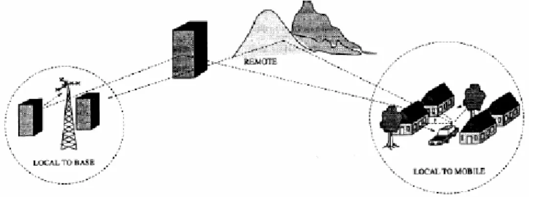
directions. The characteristic is thought as multipath propagation. The scatters of multipath propagation can be divided into three groups: local-to-mobile scatters, local-to-base scatters, and remote scatters as shown in Figure 2-2. Local-to-mobile scatters induce Doppler spread by buildings around MS. Local-to-base scatters induce angle spread by buildings around base station (BS). Remote scatters cause delay and angle spread by terrain features or high-rise buildings between BS and MS.

Considering a carrier signal transmitted in the multipath environment, the small changes in the distinctive delays by MS mobility will induce large changes in the phases of the arriving plane waves. Constructive and destructive additions of arriving plane waves reveal themselves as large variations in the phase and amplitude of the combined received signal. Because of the mobility at MS, the spatial variations in the envelope and phase of the combined received signal represent themselves as time variations. The phenomenon is called envelope fading whose rate depends on the velocity of the MS.

The directions of arriving plane waves may be significant different. A MS in the microcellular environment is usually surrounded by local scatters, so that the plane waves will arrive from different directions sometimes without line of sight (LOS) components. The assumption at MS is modeling as isotropic scattering which the plane waves arrive from all direction with equal probability. In the other hand, the BS antennas are only moderately evaluated above the local scatters.

Sometimes, multipath-fading is called as fast fading with short-term signal variations for distinguishing it from shadowing effect, which exhibits itself as the long-term signal variations of the mean envelope over the distance. The difference can be showed in Figure 2-3. Path loss predicts the transmitted power decays with distance from a BS. The researches proposed by Hata [3] and Okumura [4] incurred path loss models for microcellular systems. The models can be fit in all environments

like urban, suburban, and rural areas. Recently, the works of path loss model for microcellular systems have been suggested. The COST231 [5] model was proposed for urban areas and microcellular systems.

Figure 2-2: Scatters of Multipath propagation

2.1 Large Scale Propagation Model

Large scale fading caused by shadowing effects or natural features is also called large scale fading. Typically, it is modeled by using log-normal distribution in signal level. When the coherence time of the channel is relatively large to the delay of the channel, large scale fading arises. The amplitude and phase varied by the channel can be thought as constant over the period. The attenuation of transmitted signal power for received signal can be predicted by propagation models. Propagation models which predict the mean signal strength for an arbitrary transmitter-receiver (T-R) separation distance are of great use to predict the coverage area of transmission. Propagation models are divided into three types: free space model, path loss model, and path loss model with shadowing. We will introduce these types in the following section.

2.1.1 Free Space Model

The free space model is used to predict the received signal strength when the propagation environment is clear, unobstructed line-of-sight (LOS). There are several applications such as Satellite and microwave line-of-sight radio link for free space model. We can model the free space model by using Friis free space equation:

( ) ( ) 2 2 2 4 r t r t P d G G P d L λ π = ⋅ ⋅ ⋅ (2-1)

where P is the transmitted power, _t P d is the received power which is a function _r( ) of separation distance, G and _t G are the transmitter and receiver antenna gain _r respectively, d is the T-R separation distance, λ is the carrier wavelength, and L is the system loss factor with constrained condition: L ≥ . The factor L is affected 1 by transmission line attenuation, filter losses, and antenna losses. For the special case of L = , indicate no loss in the hardware of the communication system. In the free 1

space, the coverage is able to reach 10km per 20dB decay [6].

2.1.2 Path Loss Model

For common wireless communications, the relationship of transmitted path loss and T-R separation can be expressed as [7]:

( ) 0 _. n d PL d d ⎛ ⎞⎟ ⎜ ⎟ ∝ ⎜ ⎟_{⎜ ⎟⎜⎝ ⎠} (2-2)

The relationship can be reformulated as:

( )

( )

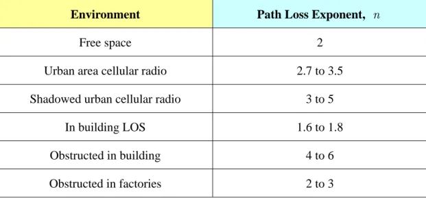
0 0 , dB 10 log d PL PL d n d ⎛ ⎞⎟ ⎜ ⎟ = + _{⎜ ⎟⎜ ⎟} ⎜⎝ ⎠ (2-3)

where PL is the average path loss, d is the T-R separation distance, n is the path loss exponential which is related to the measurement environment listed in Table 2-1 [8], and d is the reference distance. Typically, the value of ₀ d is referred as 1 km ₀ for large cells, 100 m for microcells, and 1 m for indoor channels. Because mobile communication system always works in the urban area, the coverage is about 10 km per 40 dB.

Table 2-1: Path loss exponential for different environments

Environment Path Loss Exponent, n

Free space 2

Urban area cellular radio 2.7 to 3.5 Shadowed urban cellular radio 3 to 5

In building LOS 1.6 to 1.8

Obstructed in building 4 to 6

Hata model is one of famous path loss models for describing the measure environment such as: urban, suburban, and rural area. The formulation of Hata model can be described as:

( )

, ( ) 69.55 26.16 log 13.82 log (44.9 6.55 log )log urban c b m b PL dB f h a h h d = + − − + − (2-4)

where f is the carrier frequency which is valid from 150 MHz to 1500 MHz, _c h _b and is the BS antenna height which is valid from 30m to 120m, h_m is the MS antenna height which is valid from 1m to 10m , and d is the T-R separation distance in kilo meters, and a h

( )

_m is the correlation factor for effective mobile antenna height. The correlation factor a h

( )

_m will be different from measure environments. For small to medium city,

( )

_m (dB) (1.1log _c 0.7) _m

(

1.56 log _c 0.8

)

_.

a h = f − h − f − (2-5)

For large city,

( )

( )

(

)

( )

( )

(

)

2 2 . dB 8.29 log1.54 1.1 for 300 MHz dB 3.2 log11.75 4.97 for 300 MHz m m c m m c a h h f a h h f = − ≤ = − ≥ (2-6)

The Equation 2-4 is the general case, the model can modify to different measure areas and carrier frequency range. For different measure areas, the path loss model is

(

)

2

2 log /28 5.4 suburban urban c

PL =PL − f − in the suburban area. In the open rural

areas, the model is PL_rural =PL_urban −4.78 log

(

f_c/28

)

2−18.33 logf_c −40.98. The formulation of Hata model extending to 2 GHz can be shown as follows:

( )

( )

(

)

46.3 33.9 log 13.82 log + 44.9 6.55 log log urban c b m b M PL dB f h a h h d C = + − − − + (2-7)

where f is valid from 1500 MHz to 2000 MHz, d is the transmitted distance _c which is valid from 1 km to 20 km, and C is 0 dB for medium sized city and _M

suburban areas and 3 dB for metropolitan centers.

2.1.3 Path Loss Model with Shadowing Effect

The path loss model with shadowing effect is used when arriving plane wave travels through different obstructions such as buildings, tunnels, hills, trees, etc. The received signal R is described by log-normal distribution, for r > : 0

( ) 1 (ln )2/2 2_, 2 r m p r e r σ πσ − − = (2-8)

where m and σ are the mean and standard deviation of the logarithm of the variable r .

Therefore, the path loss model with shadowing effect could be expressed in terms of PL plus a random variable X_σ, as follows:

( )

₀ 0 , 10 log = d PL PL d n X d PL X σ σ ⎛ ⎞⎟ ⎜ ⎟ = + _{⎜ ⎟⎜ ⎟}+ ⎜⎝ ⎠ + (2-9)

where X_σ is denoted as a zero-mean Gaussian distribution random variable (dB) with standard deviation 4-10 dB. The choice of X_σ is based on measurement environment.

2.2 Small Scale Propagation Model

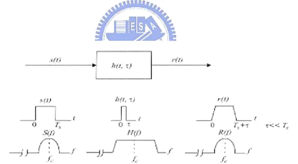
Small scale fading is used to illustrate the rapid fluctuation of the amplitude of a radio signal over a short time period, so large-scale fading can be ignored at instant time. Fast fading is caused by multipath scattering around a user and typically follows Raleigh distribution in signal envelope. The mobile radio channel is able to model as a linear filter with a time-varying impulse response [9], which can be shown in Figure 2-4. The filtering featur of the channel is induced by the summation of amplitudes and

delays of the multiple arriving plane waves at instant time.

Delay spread and coherence time are used for describing the time variation of the channel in the small-scale fading. Doppler spread is a measure of the spectral broadening induced by the variation of time rate in the mobile radio channel. It is defined as the range of frequencies over that the received Doppler spectrum is essential non-zero. In the other hand, coherence time is the time domain in opposition to Doppler spread and is used to depict the time variation of the frequency dispersive nature in the channel. It is defined as a statistical measure of the time duration over that the channel impulse response is virtually invariant.

Figure 2-4: Time-varying impulse model for a multipath radio channel

2.2.1 Flat Fading vs. Frequency-Selective Fading

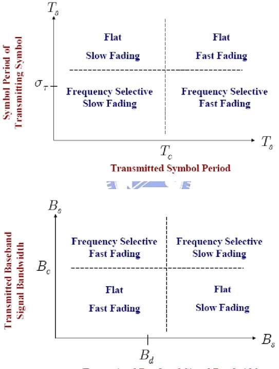
The channel model is classified mainly based on multipath time delay spread. If

bandwidth of signal B is smaller than bandwidth of channel _S B _C

(

B_S <B_C

)

and delay spread σ is smaller than symbol period _τ T _S

(

σ <_τ T_S

)

, then the model

is called flat fading channel. On the contrary, if B_S >B_C and σ_τ >T_S then the model is called frequency-selective fading channel. The flat fading channel and frequency-selective fading are also referred to as narrowband channel and wideband channel. The comparison of narrowband and wideband channel is shown in Figure 2-5.

Flat fading channel is suitable for narrowband transmission since the bandwidth of the applied signal is narrow as compared to the flat fading bandwidth of channel. It occurs when the inverse signal bandwidth (the duration of the signal) is much larger than the time spread of the propagation delays. Under the circumstance, the total frequencies of the transmitted signal will meet the same random attenuation and phase shift. The channel induces less or even no distortion for the received signal. The mobile radio channel experiences the constant gain and linear phase response over the bandwidth greater than the bandwidth of the transmitted signal. It can be shown in Figure 2-6.

In the opposition, frequency-selective fading channel used for wideband transmission occurs when the propagation delay is larger than the inverse signal bandwidth. The transmitted signal can meet different phase shifts as the distinctive propagation delays become larger. Under the circumstance, amplitude and phase distortion are introduced by the channel for the received signal. The mobile channel owns a constant gain and linear phase response over the bandwidth of the transmitted signal. It can be shown in Figure 2-7. Frequency-selective fading is due to the time dispersion of the transmitted signal, so the channel induces intersymbol interference (ISI).

Figure 2-5: Wideband channel and narrowband channel

Figure 2-7: Frequency-selective fading channel characteristics

2.2.2 Fast Fading vs. Slow Fading

The channel model is classified mainly based on Doppler spread. In other words, the channel is depending on how rapidly the transmitted baseband signal changes as compared to the rate of the channel variation. If Doppler spread B is larger than _D bandwidth of signal B _S

(

B_D >B_S

)

and symbol period T is larger than _S coherence time T_C

(

T_S >T_C

)

, then the model is called fast fading channel. On the contrary, if B_S >B_D and T_S <T_C then the model is called slow fading channel. It should be noted it will not specify whether the channel is flat fading or frequency-selective fading when channel is specified as fast or slow fading.

For the case of fast fading channel, the channel impulse response changes rapidly within the symbol duration of the transmitted signal. This causes signal distortion due to fast fading increasing Doppler spreading relative to the bandwidth of the transmitted signal, which leads to signal distortion. Fast fading only deals with the variational rate of the channel due to motion of BS [10]. For the case of the flat fading channel, it can simplify the impulse response to be the delta function. Therefore, the

flat and fast fading channel is a channel in which the amplitude of the delta function varies faster than the variational rate of the transmitted baseband signal. In the other case, the frequency-selective and fast fading channel is a channel in which the amplitudes, phases, and time delays of each multipath component vary faster than the variational rate of the transmitted baseband signal. It comes to a conclusion that fast fading only happens for very low data rates.

In the case of slow fading channel, the rate of changes of channel impulse response is slower than the transmitted signal. At this situation, the channel may be assumed to be static over one or several reciprocal bandwidth intervals. At view of frequency domain, it implies that the Doppler spread of the channel is much less than the bandwidth of the transmitted baseband signals [11].

The velocity of the mobile and the baseband signaling determines whether a signal undergoes fast or slow fading. For the summary, types of small-scale fading and their characteristics are shown in Figure 2-8 and Figure 2-9.

2.2.3 Doppler’s Effect

In the wireless mobile communications, the angles of arriving plane wave are different with the direction of movement of BS occurred by transmitter, receiver, and environment mutually shift. The phenomenon is called Doppler spread, also called Doppler shift.

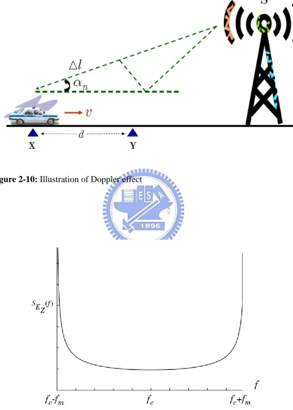
The receiving antenna is move along the path with speed v from X to Y which can be shown in Figure 2-10, and the distance between X and Y is d . In the multipath channel, assume there are n arriving plane waves, phase of each arriving plane wave is φ , the angle difference of _n φ and the direction of _n movement of BS is α , time cost from X to Y is t , then the distance d can _n be derived as d = ⋅ . The electric waves are transmitted from the transmitted v t antenna S , the angle α of X is almost the same as that of Y , because S is far _n away from X and Y . The increasing distance of transmission can be defined as

cos _n

l =d α , the relationship of phase change is derived as:

, 2 2 cos _n v t l π π φ α λ λ = = (2-10)

where λ is the wavelength of carrier wave. The Doppler shift f can be derived as: _m

, 1 cos 2 m v n f t φ _α π λ = ⋅ = (2-11)

where λ is equal to C f , C is the speed of light, and / _c f is the carrier _c wavelength. The common Doppler spectrum is U-shaped spectrum which is shown in Figure 2-11. The maximum Doppler shift occurs as arriving angle is as the same as the direction of mobility, such as α_n = , then 0 f_d =v λ/ .

Figure 2-10: Illustration of Doppler effect

2.3 Rayleigh Fading in Channel Propagation

Rayleigh distribution is commonly used to describe the statistical time varying feature of the received envelope of a flat fading signal. Envelope of the sum of the two quadrature Gaussian noise signals follows Rayleigh distribution. If there is LOS component in the multipath signals, it should be modeled as Ricean distribution.

All the arriving plane waves from random scattering direction are intergraded by the receiver antenna. According to central-limit theorem and assume there are enough plane waves and no LOS components exist, the amplitudes of in-phase and quadrature phase components obey zero-mean Gaussian distribution and the phases follow uniform distribution. It is the mathematical character of Rayleigh fading channel.

Let’s derive Rayleigh distribution completely. First, consider a carrier signal S with an amplitude A at a frequency w : ₀

(

_{0 .}

)

exp

S =A jw t (2-12)

In the receiving terminal, the received signal S is the sum of N arriving plane _r waves, which can be described as

(

₀

)

(

₀

)

1 , exp exp N r i i i S a j w t r j w t = ⎡ ⎤ ⎡ ⎤ =

_∑

_⎣ +θ _⎦ = _⎣ +θ (2-13) _⎦

where r is the envelope of receiving signal and θ is the random phase. We can define the term rexp( )jθ in Equation (2-13) to be

( ) _,

1 1

exp N _i cos _i N _i sin _i

i i r j a j a x jy = = =

_∑

+

_∑

= + θ θ θ (2-14) where 1 cos cos N i i i x a r = =

_∑

θ = θ and 1 sin sin N i i i y a r =

=

_∑

θ = θ are derived. The individual amplitudes a are random and the phases _i θ_i have a uniform distribution. According to the central limit theorem, when N is very large, it can be assumed that

2 2 2 .

x = y =

σ σ σ (2-15)

Due to x and y are independent random variables, the joint distribution ( , ) p x y is ( ) ( ) ( ) 2 2 2 2 . 1 , exp 2 2 x y p x y =p x p y = ⎛⎜⎜_⎜− + ⎞⎟⎟_⎟⎟ ⎜⎝ ⎠ πσ σ (2-16)

The distribution p r( ,θ) can be formulated as a function of p x y : ( , ) ( , ) ( , )_, p r θ = J p x y (2-17) where J is defined as cos sin sin cos . / / / / x r x r J r r y r y ∂ ∂ ∂ ∂ − ≡ = = ∂ ∂ ∂ ∂ θ θ θ θ θ θ (2-18)

Therefore, the distribution can be reformulated as

( ) 2₂ . , exp 2 2 r r p r = ⎛⎜⎜_⎜− ⎞⎟⎟_⎟⎟ ⎜⎝ ⎠ θ πσ σ (2-19)

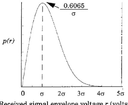
Thus, the Rayleigh fading has a probability distribution function (PDF) :

( ) ( ) _, , otherwise 2 2 2 2 0 exp 0 2 , 0 r r r p r p r d ⎧ ⎛ ⎞ ⎪ _⎟ ⎪ ⎜_{− ⎟ ≥} ⎪ ⎜_{⎜ ⎟} ⎪⎪ _⎜⎝ ⎟_⎠ = = ⎨ ⎪⎪ ⎪⎪⎪⎩

∫

π θ θ σ σ (2-20) ( ) 1 , - < < _, 2 p θ = π θ π π (2-21)

where r is received signal envelope voltage and σ is the average power of the 2 received signal, which can be shown in Figure 2-12. Assume the probability that the envelope of the received signal does not exceed a specified value R is given by the corresponding cumulative distribution function (CDF) :

( ) ( ) ( ) 2 2 0 1 exp ₂ R R P R =p r ≤R = p r dr = − ⎛⎜⎜_⎜− ⎞⎟⎟_⎟⎟ ⎜⎝ ⎠

∫

_σ (2-22)

Figure 2-12: Rayleigh PDF

2.4 Wide Sense Stationary Uncorrelated

Scattering Channels

Wide sense stationary (WSS) channels have fading statistics that remain constant over short time period. It implies that the correlation functions of channels depend on the time difference t . That can be illustrated that WSS channels give rise to scattering with uncorrelated Doppler shifts.

Uncorrelated scattering (US) channels are described by an uncorrelated attenuation and phase shift with paths of different delays. Bello suggested that US channels are wide sense stationary in the frequency domain so that the correlation functions depend on frequency difference f [12].

kind of multipath-fading channel. This channel displays uncorrelated scattering in time-delay and Doppler shift. Radio channels are always modeled as WSSUS channels. As regarding WSSUS channels, the correlation functions have singular behavior in time delay and Doppler shift.

2.5 Computer Simulations

For the discussion of the Doppler effect, we use the U-shaped Doppler spectrum defined in Jakes model. The Doppler spectrum in Jakes model is defined as :

( )

[

]

_. 2 1.5 , , 1 m m c m m S f f f f f f f f = ∈ − ⎛ _{− ⎟}⎞ ⎜ _⎟ − ⎜_{⎜⎜⎝ ⎟⎟} ⎠ π (2-23)

In Figure 2-13, We assume f =_c 1000Hz , Hzf =_m 50 , and sampling frequency f =_s 0.1Hz. The Doppler spectrum is U-shaped and symmetrical with f . _c As well as Figure 2-14, we change the Doppler shift such as f =_m 5 Hz. It can come to a conclusion that the value of Doppler shift will affect the shape of Doppler power spectrum. In other words, the slow velocity will make the Doppler power spectrum more centralize with f . _c

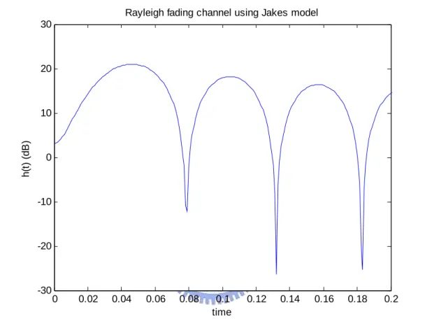
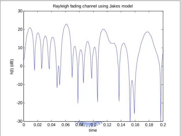
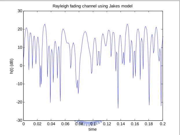
From the standpoint of fading channel using Jakes model, we assume sampling time T =_s 1msand number of subpaths N = . We set the different values of 4 Doppler shift f =_m 10, 50, and 100 Hz in Figure 2-15, Figure 2-16, and Figure 2-17, respectively. Observing these figures, we can come to a conclusion that the coherence time T gets smaller as the Doppler shift _C f gets larger. It can justify that the _m coherence time is inversely proportional to the Doppler shift f . _m

Finally, Figure 2-18 and Figure 2-19 illustrate PDF and CDF of Rayleigh fading by assuming σ = . The peak value of Rayleigh PDF in Figure 2-18 conforms to 1 analytic value 0.6065 / σ .

950 960 970 980 990 1000 1010 1020 1030 1040 1050 0 0.05 0.1 0.15 0.2 0.25 0.3 0.35 0.4 0.45 0.5 f S E (f )

Doppler Power Spectrum

950 960 970 980 990 1000 1010 1020 1030 1040 1050 0 0.05 0.1 0.15 0.2 0.25 0.3 0.35 0.4 0.45 0.5 f S E (f )

Doppler Power Spectrum

0 0.02 0.04 0.06 0.08 0.1 0.12 0.14 0.16 0.18 0.2 -30 -20 -10 0 10 20 30 time h (t) ( d B)

Rayleigh fading channel using Jakes model

0 0.02 0.04 0.06 0.08 0.1 0.12 0.14 0.16 0.18 0.2 -30 -20 -10 0 10 20 30 time h (t) ( d B)

Rayleigh fading channel using Jakes model

0 0.02 0.04 0.06 0.08 0.1 0.12 0.14 0.16 0.18 0.2 -30 -20 -10 0 10 20 30 time h (t) ( d B)

Rayleigh fading channel using Jakes model

0 0.5 1 1.5 2 2.5 3 3.5 4 4.5 5 0 0.1 0.2 0.3 0.4 0.5 0.6 0.7 X: 1 Y: 0.6065

Received signal envelope voltage r (volts)

p(

r)

Rayleigh PDF

0 0.5 1 1.5 2 2.5 3 3.5 4 4.5 5 0 0.1 0.2 0.3 0.4 0.5 0.6 0.7 0.8 0.9 1 Rayleigh CDF

Received signal envelope voltage r (volts)

P(

r)

2.6 Summary

In this chapter, the characteristics of the radio propagation and multipath fading phenomenon have been described. For large-scale fading, average received signal power decays logarithmically with T-R separation. This phenomenon is referred to as log-normal shadowing. On the other hand, for small-scale fading, the features can be divided into two kinds of viewpoints : time and frequency. The time and frequency dispersion mechanisms in a radio channel result in four different effects, which are mostly manifested depending on the features of transmitted signal, channel, and velocity. In brief, multipath delay spread causes flat and frequency selective fading and Doppler spread causes slow and fast fading. Both influential factors are independent with the other.

Modeling of multipath fading channels is also described. Rayleigh distribution is followed by multipath fading channels. WSSUS channels are assumed when analyzing the wireless communication systems. Therefore, WSSUS channels are our goal for simulating multipath fading channels. In the following section, we will introduce Jakes model briefly use the Doppler spectrum of Jakes for common.

Chapter 3

Rayleigh Fading Channel Simulators

for SISO System

Accurate and fast fading channel simulator is an essential scheme under realistic channel conditions. The new methodologies for efficient simulation of digital communications over Rayleigh fading under the assumption of wide-sense-stationary uncorrelated-scattering (WSSUS) channel are proposed. Common models for simulating fading channel can be divided into three types: direct form, modified Jakes, and Karhunen-Loeve (K-L) expansion models.

In the direct form model, channel is a discrete-time lowpass-equivalent channel impulse response (CIR) with a large number of coefficients. The simplest method for simulating Rayleigh fading is to feed white Gaussian noise (WGN) to a digital filter matched to the respective fading spectrum [13].

For the modified Jakes model, it is widely accepted for the simulation of wireless communication channels. The independent Rayleigh fader uses sum-of-sinusoids for simulations, and its statistical characteristics can approach the desired ones. However in this method, its major disadvantage is high computational complexity and how to provide the multiple uncorrelated fading waveforms. In the K-L expansion model, frequency-selective fading channel is derived from K-L expansion. Under the same mean-square error condition, the number of terms needed by the truncated K-L

expansion is less than that of a series expansion produced by the discrete-path approximation of the channel [14].

The organization of this section is as follows. Section 3.1 describes direct form model. The modified Jakes model and our proposed method using different mathematical forms for random phase are derived in Section 3.2. Section 3.3 develops an efficient K-L expansion model and compares the performance with modified Jakes model. Finally, the method accuracy is demonstrated by computer simulations in Section 3.4 and summary is given in Section 3.5.

3.1 Direct Form Model

Several authors have proposed some methods to modify the accuracy. Komninakis [15] showed that the simulator contains a fixed IIR filter followed by a variable polyphase interpolator, to accommodate different Doppler rates. The IIR filter was designed using an iterative optimization schemes that is more generally applicable and can be used to approximate any given magnitude frequency response. Fenchtel [16] found that a new simulator applied for linear amplitude/phase modulation and linear fading channels including Nyquist filtering .It is shown to be a good approximation to the conventional model in the case of tight rolloff factors

Channel having quasi- or truly continuous delay profiles can now properly illustrated at significantly reduced computational complexity. Furthermore, the new simulator leads to the lowest level of complexity being achieved for the prevailing channel and noise conditions on a particular channel. In this section, we will have more illustrations for the basic idea of direct form method.

Direct form method is a popular kind of Rayleigh fading simulation. In which, using the concept of in-phase and quadrature modulation paths to produce a simulated signal with spectral and temporal characteristics is very close to measured data.

The basic process for simulating Rayleigh fading is shown in Figure 3-1:

∑

( ⋅ )2

( ⋅ )2

⋅

x t

( )

Figure 3-1: Frequency domain implementation of a Rayleigh fading simulator at baseband for narrowband system

To carry out the simulator shown in Figure 3-1, the following steps are used:

Step1: Specifying the number of frequency domain sample points N to represent the maximum Doppler shift f , Doppler power spectral density _m S_Ez( )f can be expressed as follows : ( ) 2 , 1.5 = - 1-Z E c m m S f f f f f π ⎛⎜⎜_⎜ ⎞⎟⎟_⎟⎟ ⎜⎝ ⎠ (3-1) where m

f : the maximum Doppler frequency

f : the carrier frequency of the scattered signal _c

Step2: The frequency spacing is calculated as Δf=2 /f_m (N - 1) between each spectral lines, where time duration of a fading waveform is 1/ f .

Step3: Complex Gaussian random variables are generated for each component of /2

Step4: Assigning the conjugating positive frequency values at negative frequency, the negative frequency components are constructed.

Step5: The in-phase and quadratrue noise sources multiply with S_EZ ( )f , respectively.

Step6: Operating the inverse fast Fourier transform (IFFT) on the resulting frequency domain signals from the in-phase and quadrature components to get two length N time series, the squares of each signal point in time is added to create an N -point time series.

Step7: Taking the square root of the sum of obtained in Step6, a N -point time series of a simulator of Rayleigh fading signal will be got.

The method mentioned above is used under the condition of flat fading (frequency nonselective fading) in narrowband system. If we want to implement frequency selective fading in wideband system, just need to consider path gain and propagation time delay settings. We will have complete description in Chapter 4.

3.2 Jakes Model and Modified Jakes Models

Rayleigh fading channels are widely using sum-of-sinusoids based on Jakes model method for simulating mobile radio channel. Many different models [19]-[24] focus on approximating the random process by the superposition of a finite number of properly selected sinusoids. Generally, these models can be classified as either statistical or deterministic. The statistical models leave at least one of parameter sets (path amplitudes, random phases, or Doppler frequencies) as time-variant random variables. In contrast, the deterministic models have fixed parameter sets for all simulation trials. The deterministic properties are relatively popular because of their

simplicity.

3.2.1 Clarke Model and Jakes Model

Many approaches have been suggested for modeling Rayleigh fading waveforms. Clarke was the first author to propose the well know mathematical reference model for Rayleigh fading channel [17]. A simplified version of Clarke’s model proposed by Jakes has been widely used in three decades [18].

Clarke’s reference model defines the complex faded envelope g t as: ( )

( ) ( ) ( ) 1 ( cos ) 0 , m n n N _{j w t} c s n n g t g t jg t − C e α +φ = = + =

_∑

(3-2) where

N : the number of propagation paths of a single fader

m

w : the maximum Doppler frequency in radius

n

C : the path gain

n

α : the thn angle of arrival which is uniformly distributed on the interval [−π π, )

n

φ : the initial phase associated with the thn propagation path which is uniformly distributed on the interval [−π π, ).

By the Central Limit Theorem, the real part g t_c( )=Re{g t( )} and the imaginary part g t_s( )= Im{g t( )} of the complex faded envelope can be approached as Gaussian random process when N → ∞ . Assuming a two dimensional (2-D) isotropic scattering environment, the autocorrelation and cross-correlation function can be described as below:

( )

[

( ) ( )

]

₀

(

)

c c

g g c c m

( )

[

( ) ( )

]

₀

(

)

s s g g s s m R τ =E g t g t +τ =J w τ (3-4) ( ) ( ) 0 c s s c g g g g R τ =R τ = (3-5) ( ) 1 ( ) ( ) ₀

(

)

2 gg m R τ = E g t g t⎡_⎣ ∗ +τ ⎤_⎦ =J w τ (3-6) ( )

(

)

2 2 4 4 ₀2 _{m ,} g g R τ = + J w τ (3-7) where [ ]

E ⋅ : the statistical exception operator

J ⋅ : the zero-order Bessel function of the first kind. ₀( )

Without the loss of generality, we can set 2

0 1 N n n E C = ⎡ _{⎤ =} ⎢ ⎥ ⎣ ⎦

∑

and E =₀ 2. The

probability density function (PDF) of the fading envelope g t and its phase ( )

( ) ( ) ( ) 1 tan c g c g t t g t θ = − ⎛⎜⎜_⎜ ⎞⎟⎟_⎟⎟

⎜⎝ ⎠ can be given by:

( ) 2 2_{, 0} x g f x = ⋅x e− x ≥ (3-8) ( ) 1 , [ , ) 2 g f_θ φ φ π π π = ∈ − (3-9)

According to the above equation, the ideal fading envelope g t is Rayleigh ( ) distribution and the phase θ_g( )t is uniformly distribution.

Jakes Model derived well-known deterministic simulation model for Rayleigh fading channels, based on Clarke’s reference model and by selecting C_n =1/ N ,

2 /

n n N

α = π , and φ = for _n 0 n =1,2, ,N . The N fading waveforms of a single fader can be reduced to N₀ =(N −2 / 4) . The implementation is shown in Figure 3-2. The normalized low-pass process of this model is given by

( ) _c( ) _s( ) g t =g t +jg t (3-10) ( ) 0

(

)

0 2 cos N c n n n g t a w t N ₌ =

_∑

(3-11)

( ) 0

(

)

0 2 cos N s n n n g t b w t N ₌ =

_∑

(3-12) where N =4N₀+ , and 2 0 , 0 2 cos , 0 2 cos 1,2, , n n n a n N β β ⎧⎪ = ⎪⎪ = ⎨_⎪ = ⎪⎪⎩ … (3-13) 0 , 0 2 sin , 0 2 sin 1,2, , n n n b n N β β ⎧⎪ = ⎪⎪ = ⎨_⎪ = ⎪⎪⎩ … (3-14) 0 0 , 0 4 , 1,2, , n n n n N N π β _π ⎧⎪ ₌ ⎪⎪ ⎪ = ⎨_⎪ = ⎪⎪ ⎪⎩ … (3-15) 0 , 0 2 cos , 1,2, , m n m w n w _n w n N N π = ⎧⎪⎪ ⎪ = ⎨_⎪ = ⎪⎪⎩ … (3-16)

Figure 3-2: Jake fading channel simulator

number of sinusoids. However, an important shortcoming in the design is that the rays experiencing the same Doppler frequency shift are correlated [19]. This causes the generating signals to be wide-sense-nonstationary. Therefore, various modifications of Jakes Model have been found in the literature.

3.2.2 Development of Modified Jakes Models

Pop and Beaulieu model [20] was suggested by removing the constraint 0

n

φ = of Jakes model and let the phases φ to be uncorrelated. Assuming there _n are M independent faders, a single fader will be composed of N waveforms which can be reduced to N as Jakes model. The th₀ k complex faded envelope (fader) can be defined as ( ) ( ) ( )

c s k k k g t =g t +jg t , where k =0,1, ,… M −1 ( )

( )

0

(

0

)

0

( )

(

)

1 4 8

cos cos cos cos cos c N k m k n m n nk n g t w t w t N β φ N ₌ β α φ = + +

_∑

⋅ + (3-17) ( )

( )

₀

(

₀

)

( )

(

)

1 , 4 8

sin cos sin cos cos

s M k m k n m n nk n g t w t w t N β φ N ₌ β α φ = + +

_∑

+ (3-18) where n

α : the thn angle of arrival which is equal to 2πn N/ m

w : the maximum Doppler frequency in radius

n

β : the phase which is equal to πn N/ ₀, for n =0,1, ,… N₀ nk

φ : the initial phase associated with the thn propagation path of the thk fader which is uniformly distributed on the interval [−π π, )

Li and Huang model [21] is an ergodic statistical model, which converges to the desired properties in a single simulation trial. The fading model is proposed by

using of asymmetrical arrival angle arrangement and appropriately chosen incident wave phases. The in-phase and quadrature components in any faders are independent, so each fading waveform will be uncorrelated. The number of fading waveforms of a single fader can be reduced to N₀ =N / 4. The thk complex faded envelope can be defined as ( ) ( ) ( ) c s k k k g t =g t +jg t , where k =0,1, ,… M −1 ( ) 0 1

(

)

0 0 1 cos cos c N I k m nk nk n g t w t N α φ − = =

_∑

⋅ + (3-19) ( ) 0 1

(

)

0 0 , 1 sin sin s N Q k m nk nk n g t w t N α φ − = =

_∑

⋅ + (3-20) where

α_nk : the thn angle of arrival in the thk fader which is equal to

00 2 n 2 k N MN π ₊ π _+α , where 0 ₀₀ 2 MN π α < < and ₀₀ MN π α ≠ I nk

φ : the initial phase of the inphase component in the thk fader which is uniformly distributed on the interval [−π π, )

Q nk

φ : the initial phase of the quadrature component in the thk fader which is uniformly distributed on the interval [−π π, )

Dent model [22] was proposed to modify Jakes model by using orthogonal Walsh-Hadamard codeword to de-correlate the multiple faded envelope. The number of fading waveforms of a single fader can be reduced from N to N₀ =N/ 4. The

th

k complex faded envelope can be defined as ( ) ( ) ( )

c s k k k g t =g t +jg t , where 0,1, , 1 k = … M − ( ) 0 ( )

( )

(

)

0 1 2

cos cos cos

c N k k n m n n n g t A n w t N ₌ ⎡ β α φ ⎤ =

_∑

×_⎣ ⋅ ⋅ + _⎦ (3-21)

( ) 0 ( )

( )

(

)

, 0 1

2

sin cos cos

s N k k n m n n n g t A n w t N ₌ ⎡ β α φ ⎤ =

_∑

×_⎣ ⋅ ⋅ + _⎦ (3-22) where ( ) k

A n : the thk Walsh-Hadamard code sequence in the thn subpath ( 1± values)

n

α : the thn angle of arrival which is equal to 2π(n−0.5 /) N

n

β : the phase which is equal to πn N/ ₀ n

φ : the initial phase associated with the thn propagation path which is uniformly distributed on the interval [−π π, )

Wu model [23] was proposed for modifying Dent model, the correlation properties are as good as Li and Huang model, which are better than those of Jakes and Dent models. However, the computational complexity of Wu model is just one half of the Li and Huang model. The number of fading waveforms of a single fader can be reduced to N₀ =N/ 4. The thk complex faded envelope can be defined as

( ) ( ) ( ) c s k k k g t =g t +jg t , where k = 0,1, ,… M −1 ( ) 0 ( )

(

)

1 1 0 0 1 cos cos c N k k m nk n n g t A n w t N α φ − = =

_∑

⋅ + (3-23) ( ) 0 ( )

(

)

1 2 _, 0 0 1 cos cos s N k k m nk n n g t A n w t N α φ − = =

_∑

⋅ + (3-24) where ( ) ( ) 1 , 2 k k

A n A n : the thk orthogonal sequence in n (± ), which satisfies 1

( ) ( ) 0 1 0 0 1, , 1 0, else , 0,1, , 1 , 1,2 N kp lq n k l p q A n A n N k l M p q − ∗ = ⎧ = = ⎪⎪ = ⎨ ⎪⎪⎩ = − =

∑

…

α : the th_nk n angle of arrival in the thk fader which is equal to 2 n 2 k

N MN

π ₊ π n

φ : the initial phase associated with the thn propagation path which is uniformly distributed on the interval [−π π, )

Zheng and Xiao model [24] is not as the same as the above models, it is a typical statistical model. They proposed an improved simulator by introducing random phase shifts in random phase shifts in the low-frequency oscillators to remove the stationary problem from Jakes model. By allowing parameter sets of amplitudes, phases, and Doppler frequencies to be independent random variables, the statistical properties converge to desired values when average over 50 to 100 simulation trials. The number of fading waveforms for simulation can be reduced to N₀ =N/ 4. The

th

k complex faded envelope can be defined as ( ) ( ) ( )

c s k k k g t =g t +jg t , where 0,1, , 1 k = … M − ( ) 0

₍

₎

_[

_]

0 1 2

cos cos cos

c N k nk m nk k n g t w t N ₌ ψ α φ =

_∑

⋅ + (3-25) ( ) 0

(

)

[

]

0 1 , 2

sin cos cos

s N k nk m nk k n g t w t N ₌ ψ α φ =

_∑

⋅ + (3-26) where nk

α : the thn angle of arrival in the thk fader which is equal to

2 n _k

N π − +π θ

k

θ : the random of the thk fader phase which is uniformly distributed on the interval [−π π, )

nk

ψ : the random phase of the thk fader which is uniformly distributed on the interval [−π π, )

k

interval [−π π, )

The above models can make a summary as Table 3-1.

Table 3-1: Summary of modern modified Jakes models

Complex Faded Envelope

Pop

and

Beaulieu

( ) ( ) ( ) ( ) ( ) ( ) ( ) ( ) ( ) 0 0 0 1 0 0 1

4 _{cos cos} 8 _{cos cos cos}

4 8

sin cos sin cos cos

N k m k n m n nk n M m k n m n nk n g t w t w t N N j w t w t N N β φ β α φ β φ β α φ = = = + + ⋅ + ⎧ ⎫ ⎪ ⎪ ⎪ ⎪ + ⎨_⎪ + + + ⎬_⎪ ⎪ ⎪ ⎩ ⎭ ∑ ∑

Li

and

Huang

( ) 0 1

(

)

0 1

(

)

0 0 0 0 1 1

cos cos sin sin

N N I Q k m nk nk m nk nk n n g t w t j w t N α φ N α φ − − = = = _∑ ⋅ + + _∑ ⋅ +

Dent

( ) ( ) ( ) ( ) ( ) ( ) ( ) 0 0 0 1 0 1

2 _{cos cos cos} 2

sin cos cos

c N k k n m n n n N k n m n n n g t A n w t N j A n w t N β α φ β α φ = = ⎡ ⎤ = ×_⎣ ⋅ ⋅ + _⎦ ⎧ ⎫ ⎪ ⎪ ⎪ _{⎡ ⎤}⎪ + ⎨_⎪ ×_⎣ ⋅ ⋅ + _⎦⎬_⎪ ⎪ ⎪ ⎩ ⎭ ∑ ∑

Wu

( ) ( ) ( ) ( ) ( ) 0 0 1 1 0 0 1 2 0 0 1 cos cos 1 cos cos N k k m nk n n N k m nk n n g t A n w t N j A n w t N α φ α φ − = − = = ⋅ + + ⋅ + ∑ ∑

Zheng

and

Xiao

( ) ( ) [ ] ( ) [ ] 0 0 0 1 0 1

2 _{cos cos cos} 2

sin cos cos

N k nk m nk k n N nk m nk k n g t w t N j w t N ψ α φ ψ α φ = = = ⋅ + + ⋅ + ∑ ∑

3.2.3 Proposed Modified Jakes Model

A novel sum-of-sinusoids Rayleigh fading model is proposed by decomposing the term of initial random phase. In accordance with Clarke’s model, we can define the thk complex faded envelope