空間統計模型選取之大樣本理論

國

立

交

通

大

學

統計學研究所

博

士

論

文

空間統計模型選取之大樣本理論

Asymptotic Theory for Geostatistical Model Selection

研 究 生：張志浩

指導教授：黃信誠 博士

共同指導：銀慶剛 博士

空間統計模型選取之大樣本理論

Asymptotic Theory for Geostatistical Model Selection

研 究 生：張志浩 Student：Chih-Hao Chang

指導教授：黃信誠 Advisor：Hsin-Cheng Huang

共同指導：銀慶剛

Co-Advisor：Ching-Kang Ing

國 立 交 通 大 學

統 計 學 研 究 所

博 士 論 文

National Chiao Tung University, Hsinchu, Taiwan for the Degree of

Doctor of Philosophy in Institute of Statistics

June 2011

Hsinchu, Taiwan, Republic of China

空間統計模型選取之大樣本理論

學生：

指導教授

共同指導

國立交通大學 統計學研究所 博士班

摘

要

在傳統迴歸模型中，模型選取的大樣本理論已被廣泛建立。然而在空間統計

迴歸模型中，使用傳統模型選取準則的選模結果並未被完善的討論及研究，尤其

當假設資料觀測空間為一固定區域而不隨著樣本增加而放大時，其大樣本理論可

以預期會與傳統的理論結果有所差異。論文中，我們在一些常規假設下，建立了

傳統模型選取準則的大樣本理論。而後在一維空間的一些例子下，我們發現這些

常規假設的成立與否不僅與樣本空間放大的速度有關，也與所選取變數在空間中

的平滑程度有緊密關係。當空間互變異函數參數未知時，我們同樣發現，參數估

計及傳統模型選取準則的大樣本理論，也與樣本空間放大的速度和所選取變數在

空間中的平滑程度有關。最後我們執行有限樣本的模擬實驗，並得到與大樣本理

論一致的結果。

ii

Asymptotic Theory for Geostatistical Model Selection

student：

Advisors：Dr.

Co-Advisor

Dr.

Institute of

National Chiao Tung University

ABSTRACT

Information criteria, such as Akaike's information criterion (AIC), Bayesian

information criterion (BIC), and conditional AIC (CAIC) are often applied in model

selection. However, their asymptotic behaviors under geostatistical regression models

have not been well studied particularly under the fixed domain asymptotic framework

with more and more data observed in a bounded fixed region. In this thesis, we

investigate two classes of criteria for geostatistical model selection: generalized

information criterion (GIC) and conditional GIC (CGIC), which include AIC, BIC,

and CAIC as special cases, under both the increasing domain asymptotic and fixed

domain asymptotic frameworks. We establish conditions under which GIC and CGIC

are selection consistent and asymptotically efficient even without assuming spatial

covariance structure to be known. These conditions are further examined for GIC and

CGIC in selecting one-dimensional geostatistical regression models with the

exponential covariance function class under various settings. For example, under the

fixed domain asymptotic framework, where some covariance parameters are not

consistently estimable, we show that selection consistency not only depends on the

tuning parameter of GIC, but also depends on smoothness of the explanatory variables

in space. In addition, under the increasing domain framework, we show that

asymptotic properties of GIC depend on the growing rates for the size of the domain.

Moreover, some numerical experiments are provided to demonstrate the finite sample

behavior of various criteria.

iii

誌

謝

回首交通大學多年的求學生涯，首先我要感謝的是黃信誠老師，在學術研

究的漫漫長路上，給了我很多大方向小細節的指導與叮嚀，也感謝老師付出了

這麼多的勞力與心力，一一糾正我散漫不經心的錯誤，為論文劃下了一個完善

的句點，並諄諄教誨的讓我謹記不至於在未來的路途上犯下重複的錯誤，以期

在研究的路上能走得更遠更踏實。同時要感謝銀慶剛老師，在研究的方向與證

明的細節上，不時的給予了非常即時的指導與建議，完善且充實了論文中的內

容，並讓我在研究過程中少走了許多彎路，得到了更多的啟發，在此特別感謝

兩位老師所給予的指導。

另外感謝在最後的口試當天，對於論文提出了寶貴的意見與建議的口試委

員： 徐南蓉教授、王維菁教授、洪慧念教授、林培生教授，進而修補了論文

中的不足之處。同時感謝所上的老師，再學校的授課過程中，讓我累積了足以

通過資格考並進而得到了博士學位的學識。

而在學校的日子中，與同學們的相處，有一起考過資格考的喜、一起沒考

過資格考的哀，也有一起舉杯八卦的樂，感謝秋婷、江村剛志、穗碧、達叔、

弘家、家群，還有最後給予我很大幫忙的健霖，或許我們離開學校的日子不一

樣，但我會珍惜我們一起相伴過的日子。也感謝在中研院擔任助理時，春樹學

長的提點，幫助我更快融入中研院的環境。最後特別感謝郭碧芬郭姐，如果沒

有郭姐，我可能會忘記考入學考，可能會忘記註冊，真的很感謝郭姐不時的即

時提醒。

最後，我要感謝我的家人，感謝爸爸、媽媽、大姐、二姐、小弟，還有兩

位姐夫，對於我的支持與包容，我知道妳們都相信我可以，只是不好意思讓大

家等這麼久，謹將此本論文與我的博士學位獻給我愛與愛我的爸媽，謝謝你們

長久以來的一路栽培，也希望在未來的人生大道中，在你們的相伴與敦促下，

繼續的分享我的酸甜苦辣。

張志浩 謹識於

國立交通大學統計學研究所

中華民國一百年六月

Contents

Contents iv

List of Tables vi

List of Figures viii

1 Introduction 1

2 Geostatistics 4

2.1 Geostatistical Models . . . 4

2.2 Variograms and Covariance Functions . . . 4

2.3 Kriging and Spatial Prediction . . . 5

2.4 Covariance Parameter Estimation . . . 7

2.5 Asymptotic Frameworks . . . 8

3 Variable Selection 11 3.1 Loss Functions . . . 12

3.2 Consistency and Asymptotic Loss Efficiency . . . 14

4 Generalized Information Criterion 16 4.1 Akaike’s Information Criterion . . . 16

4.2 Generalized Information Criterion . . . 17

4.3 Unknown Covariance Parameters . . . 18

5 Exponential Covariance Models in One Dimension 25 5.1 Polynomial Order Selection . . . 30

5.2 Spatially Dependent Regressors . . . 39

5.3 White Noise Regressors . . . 48

6 Conditional Generalized Information Criterion 56 6.1 Conditional Akaike’s Information Criterion . . . 56

6.2 Conditional Generalized Information Criterion . . . 70

7 Simulations 74 7.1 Experiment I: Polynomial Order Selection . . . 74

7.2 Experiment II: Spatially Dependent Regressors . . . 75

8 Summary and Discussion 84

8.1 Zeros of Covariance Parameters . . . 84

8.2 Other Covariance Structures . . . 84

8.3 Sampling Designs . . . 84

8.4 Continuous Functions as Explanatory Variables . . . 85

9 Appendix: Proofs 86

List of Tables

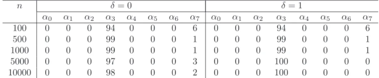
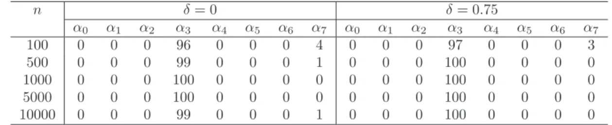
7.1 Frequencies of models selected by GIC with two tuning parameter values of λ for Experiment I based on 100 simulation replicates. . . . 75

7.2 Candidate models for Experiments II and III. . . 78

7.3 Frequencies of models selected by BIC for Experiment II with {σ2

η, κη, σ²2} known based on 100 simulation replicates. . . 78

7.4 Frequencies of models selected by BIC for Experiment II with {σ2

η, κη, σ²2} unknown based on 100 simulation replicates. . . 78

7.5 Frequencies of models selected by BIC for Experiment III with {σ2

η, κη, σ²2} known based on 100 simulation replicates. . . 81

7.6 Frequencies of models selected by BIC for Experiment III with {σ2

η, κη, σ²2} unknown based on 100 simulation replicates. . . 81

List of Figures

1.1 Locations of monitoring stations in Taoyuan, Hsinchu and Miaoli counties in Taiwan Air Quality Monitoring Network. . . 2

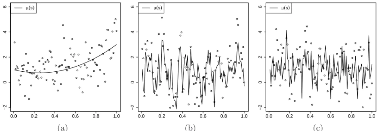
7.1 Mean functions and simulated data from (a) Experiment I, (b) Experiment II, and (c) Experiment III for δ = 0 and n = 100. . . . 75

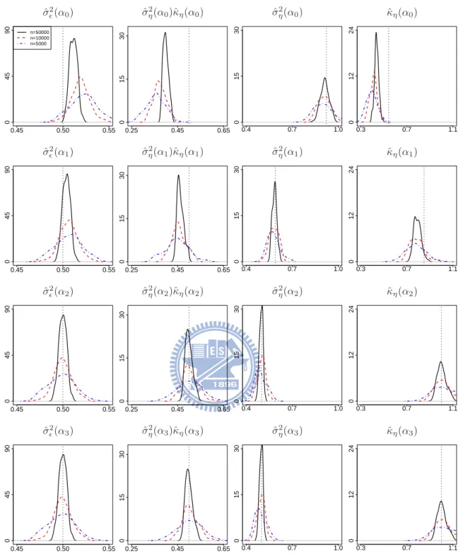
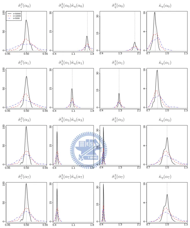
7.2 Probability density functions for the ML estimates of covariance parameters in Experiment I with δ = 0 based on 100 simulation replicates, where the solid lines, the dashed lines, and the dot-dashed lines correspond to n = 50000, 10000, 5000, respectively, and the vertical dotted lines correspond to the convergence values of the ML estimates. Some density functions have support outside displayed regions. . . 76

7.3 Probability density functions for the ML estimates of covariance parameters in Experiment I with δ = 0.75 based on 100 simulation replicates, where the solid lines, the dashed lines, and the dot-dashed lines correspond to n = 50000, 10000, 5000, respectively, and the vertical dotted lines correspond to the convergence values of the ML estimates. Some density functions have support outside displayed regions. . . 77

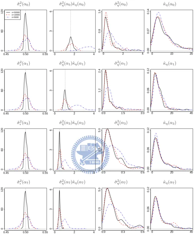
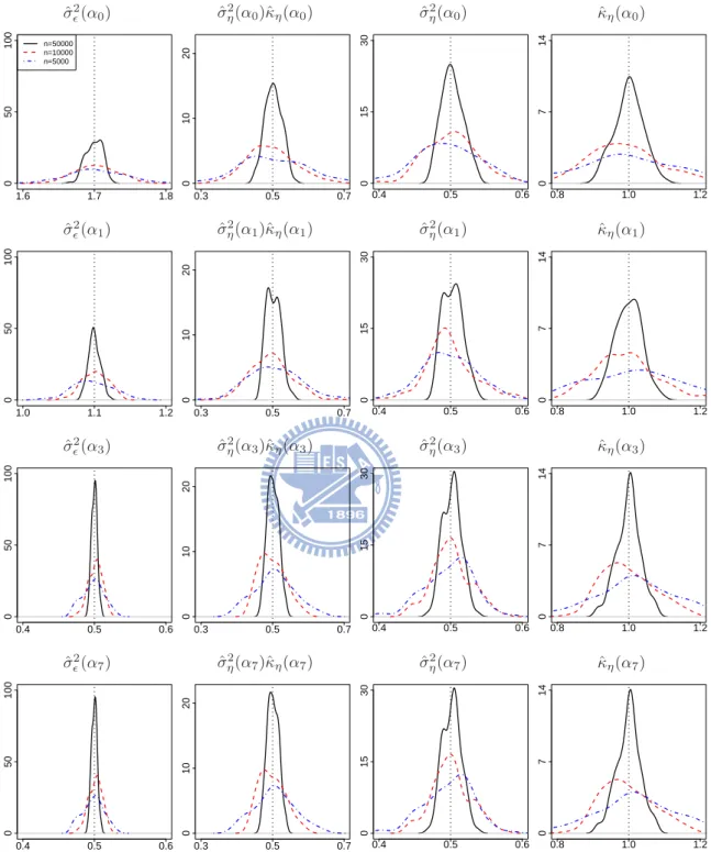
7.4 Probability density functions for the ML estimates of covariance parameters in Experiment II with δ = 0 based on 100 simulation replicates, where the solid lines, the dashed lines, and the dot-dashed lines correspond to n = 50000, 10000, 5000, respectively, and the vertical dotted lines correspond to the convergence values of the ML estimates. Some density functions have support outside displayed regions. . . 79

7.5 Probability density functions for the ML estimates of covariance parameters in Experiment II with δ = 0.75 based on 100 simulation replicates, where the solid lines, the dashed lines, and the dot-dashed lines correspond to n = 50000, 10000, 5000, respectively, and the vertical dotted lines correspond to the convergence values of the ML estimates. Some density functions have support outside displayed regions. . . 80

7.6 Probability density functions for the ML estimates of covariance parameters in Experiment III with δ = 0 based on 100 simulation replicates, where the solid lines, the dashed lines, and the dot-dashed lines correspond to n = 50000, 10000, 5000, respectively, and the vertical dotted lines correspond to the convergence values of the ML estimates. Some density functions have support outside displayed regions. . . 82

7.7 Probability density functions for the ML estimates of covariance parameters in Experiment III with δ = 0.75 based on 100 simulation replicates, where the solid lines, the dashed lines, and the dot-dashed lines correspond to n = 50000, 10000, 5000, respectively, and the vertical dotted lines correspond to the convergence values of the ML estimates. Some density functions have support outside displayed regions. . . 83

Chapter 1

Introduction

More and more spatial data are collected in this world. In many problems, several variables are measured at some locations over a region in space, and it is of interest to predict a variable at some locations, where measurements may or may not be taken, based on all data available in the region. We can formulate the problem as a geostatistical regression problem by treating the variable of interest as the response and regressing it with other (explanatory) variables while accounting for spatial dependencies. However, inference and prediction generally depend on how explanatory variables are chosen, which if not chosen properly, may lead to poor inference and prediction, particularly when the number of explanatory variables is large. Clearly, model selection problem is essential in geostatistics. For example, suppose that we are interested in knowing ground-level ozone concen-trations for a region consisting of Taoyuan, Hsinchu and Miaoli in Taiwan based on data measured at some monitoring stations in Taiwan Air Quality Monitoring Network (see Figure 1.1). At each monitoring station, we collect hourly ozone concentrations together with some explanatory variables, including ozone precursors (such as nitrogen oxides and hydrocarbons), meteorological variables (such as wind speed and wind direction, tem-perature, mixing height, humidity and rainfall), altitude, population, etc. It is of inter-est to identify influential explanatory variables for ozone concentrations, and to predict ozone concentrations for the whole region by applying a geostatistical regression model. Although lower altitudes, lower wind speeds, and higher temperatures are expected to associate with higher ozone concentrations, some other variables may or may not have effects on ozone concentrations. Removing unrelated variables, while retaining impor-tant variables, will allow one to reduce estimation variability, thereby increase prediction accuracy.

There are two different asymptotic frameworks in geostatistics. One is called the in-creasing domain asymptotic framework, where the observation region grows with the sam-ple size. The other is called the fixed domain asymptotic (or infill asymptotic) framework, where the observation region is bounded and fixed. It is known that these two frameworks lead to possibly different asymptotic behaviors on covariance parameter estimation, and hence are also expected to produce different asymptotic behaviors on model selection. In general, asymptotic behaviors under the increasing domain asymptotic framework are more standard. For example, the maximum likelihood (ML) estimates of covariance pa-rameters are typically consistent and asymptotically normal (Mardia and Marshall 1984). In contrast, not all covariance parameters can be consistently estimated under the fixed domain asymptotic framework even for a simple one-dimensional example with the sta-tionary exponential covariance model (Ying 1991). The readers are refereed to Stein

Figure 1.1: Locations of monitoring stations in Taoyuan, Hsinchu and Miaoli counties in Taiwan Air Quality Monitoring Network.

(1999) for more details regarding fixed domain asymptotics.

There are many model selection methods that have been applied in geostatistical model selection, such as Akaike’s information criterion (AIC, Akaike 1973), Bayesian information criterion (BIC, Schwartz 1978), the generalized information criterion (GIC, Nishii 1984), and cross validation. Note that GIC contains a tuning parameter, which includes both AIC and BIC as special cases. Although asymptotic properties of these selection methods have been well studied in linear regression and time series model selection (e.g., Shao 1997; McQuarrie and Tsai 1989), they have not been well established for geostatistical model selection. In fact, there are only limited results available partly because asymptotic properties under the fixed domain asymptotic framework are generally nonstandard and difficult to handle. Hoeting et al. (2006) provided some heuristic arguments for AIC in geostatistical model selection under the assumption that the variable of interest is observed with no measurement error. They show via a simulation experiment that spatial dependence has to be considered, which if ignored, may lead to unsatisfactory results. For linear mixed-effect models, Pu and Niu (2006) provided conditions under which GIC is selection consistent. In addition, Vaida and Blanchard (2005) developed a criterion for linear mixed model selection, called the conditional Akaike’s information criterion (CAIC). This criterion provides unbiased estimation of the mean squared prediction error, which appears to be more suitable than AIC for geostatistical model selection when spatial prediction is of main interest. Huang and Chen (2007) developed a general technique of estimating the mean squared prediction error for a general spatial prediction procedure, in which a concept called generalized degrees of freedom is used to provide an almost unbiased estimate. Their method is applicable to select among arbitrary spatial prediction methods, and is shown to achieve some asymptotic efficiency result.

In this thesis, we first study GIC for geostatistical model selection. Then we propose a new criterion, called conditional GIC (CGIC), which includes CAIC as a special case.

Major accomplishments are listed in the following:

1. Asymptotic properties of GIC under both the fixed domain asymptotic and the increasing domain asymptotic frameworks are established under some regularity conditions.

2. Asymptotic properties of CGIC under both the fixed domain asymptotic and the increasing domain asymptotic frameworks are established under some regularity conditions.

3. The above regularity conditions are explicitly checked for some examples in the one-dimensional space with various forms of explanatory variables under the exponential covariance model corresponding to the Ornstein-Uhlenbeck process (Uhlenbeck and Ornstein, 1930).

We shall show that asymptotic behaviors of these criteria are related to how fast the domain increases with the sample size. In addition, some nonstandard behaviors of these criteria under the fixed domain asymptotic framework will be highlighted. For example, under the fixed domain asymptotic framework, GIC and CGIC fail to identify the correct set of polynomial variables consistently regardless of which tuning parameters are chosen. On the other hand, both BIC and CBIC are selection consistent when candidate variables are generated from either white-noise processes or some zero-mean spatial dependent processes.

We shall start by developing asymptotic results under known covariance parameters, and then allowing them to be unknown. However, under the fixed domain asymptotic framework, ML estimates may converge to nondegenerate distributions. In this situation, general asymptotic properties are very difficult to develop even for parameter estimation. Therefore, we shall focus only on some examples of geostatistical models defined over the one-dimensional space with the exponential covariance model.

The thesis is organized as follows. Chapter 2 gives a brief introduction of geostatistics, including various spatial covariance models, various spatial prediction and parameter esti-mation methods. In Chapter 3, we introduce the variable selection problem and consider two loss functions for comparing among different methods. In Chapter 4, some asymp-totic properties of GIC are established under some regularity conditions. These conditions are further verified by some examples in the one-dimensional space with the exponential covariance model under either known or unknown covariance parameters in Chapter 5. Chapter 6 is devoted to CGIC and its asymptotic properties. Chapter 7 provides some simulation examples for comparing among various model selection criteria. Some con-clusions and discussion regarding future research directions are provided in Chapter 8. Finally, the appendix contains proofs for all lemmas and propositions.

Chapter 2

Geostatistics

This chapter provides a brief introduction to geostatistics, including geostatistical models, spatial prediction, parameter estimation, and the two asymptotic frameworks.

2.1

Geostatistical Models

Consider a spatial process {S(s) : s ∈ D} of interest defined over a region D ⊂ Rd _with

d ∈ N ≡ {1, 2, . . . }. Suppose that we observe data {(x(si), Z(si)) : i = 1, . . . , n} at locations si ∈ D, where

x(si) = (1, x1(si), . . . , xp(si))0, (2.1)

is a p-vector of explanatory variables observed at si ∈ D, and Z(si) is the corresponding response variable observed according to the following measurement equation:

Z(si) = S(si) + ²(si); i = 1, . . . , n,

and {²(si) : i = 1, . . . , n} are white-noise variables corresponding to measurement errors with variance σ2

². The spatial process S(·) is further decomposed into a linear combination of explanatory variables x(·)0_{β and a zero-mean spatial dependent process η(·):}

Z(si) = x(si)0β + η(si) + ²(si); si ∈ D, i = 1, . . . , n. (2.2) In general, η(·) is assumed to be L2_{-continuous (i.e., E(η(s)−η(s}0₎₎2 _{→ 0 as ks−s}0_{k → 0)} with its spatial dependence structure described by a variogram model or a covariance model (Section 2.2). The goal is either to make inference on β or more often to predict

{S(s) : s ∈ D} based on data Z ≡ (Z(s1), . . . , Z(sn))0. Commonly used loss functions for spatial prediction includeR_s∈D¯¯ ˆS(s) − S(s)¯¯2ds and

n X i=1 ¡_ˆ S(si) − S(si) ¢₂ , where ˆS(s)

denotes a generic predictor of S(s) at s ∈ D.

2.2

Variograms and Covariance Functions

In geostatistical literature, spatial dependence is commonly described using a variogram, defined as

The function γ∗_{(·, ·) is usually called the semivariogram. Clearly, γ}∗_{(s, s}0_{) ≥ 0 and}

γ∗_{(s, s) = 0, for s, s}0 _{∈ D. A spatial process S(·) is said to be intrinsically} station-ary if it has a constant mean: E(S(s + h) − S(s)) = 0, and its variogram can be written as

2γ(h) ≡ 2γ∗_{(s + h, s) = E(Z(s + h) − Z(s))}2_,

for any pairs s and s + h ∈ D. Note that the function 2γ(h) does not depend on s. Spatial dependence can also be described using a covariance function:

C(s, s0) ≡ cov(S(s), S(s0)); s, s0 ∈ D.

Similar to an intrinsically stationary process, a spatial process S(·) is said to be second-order stationary if E(S(s + h) − S(s)) = 0 and its covariance function can be written as:

K(h) = C(s, s + h) = cov(S(s), S(s + h)),

independent of s, for any s, s + h ∈ D. Clearly, K(h) = K(−h), and |K(h)| ≤ K(0) = var(S(s)), for s ∈ D. Note that a second-order stationary process is an intrinsically stationary process with γ(h) = K(0) − K(h), but not necessary vice versa. For example, a Brownian motion is an intrinsically stationary process, but not a stationary process, because its variance is not a constant (see Cressie 1993).

In addition, a second-order stationary process is said to be isotropic if K(h) depends on h only through khk, where k · k is the L2 _{norm. In what follows, we introduce some} isotropic stationary covariance function classes commonly used in the literature. The exponential covariance class is given by:

K(h) = σ2_ηexp(−κηkhk), (2.3) where σ2

η > 0 and κη ≥ 0 is a range parameter. The Gaussian covariance class is given by:

K(h) = σ2

ηexp(−κηkhk2), (2.4)

where σ2

η > 0 and κη ≥ 0 is a range parameter. The Mat´ern covariance class (Mat´ern 1986) is given by: K(h) = σ 2 η(κkhk)ν Γ(ν)2ν−1 Kν(κηkhk), (2.5) where σ2

η > 0, κη ≥ 0 is a range parameter, ν > 0 is a smoothness parameter, and Kν is the modified Bessel function of the second kind with order ν (Abramowitz and Stegun 1965). Note that the Mat´ern covariance class contains the exponential covariance class as a special case when ν = 0.5. It also reduces to the Gaussian covariance class as ν → ∞.

2.3

Kriging and Spatial Prediction

Spatial prediction is commonly called kriging in geostatistics, which utilizes spatial depen-dence structure to interpolate or smooth the surface of a spatial stochastic process based on (noisy) data observed at some locations in space. It is named after a South African mining engineer, Daniel Gerhardus Krige (1951), who pioneered the field of geostatistics. In this section, we are going to introduce several kriging methods derived under different circumstances.

Simple Kriging

Suppose that we observe data Z = (Z(s1), . . . , Z(sn))0 _{according to (2.2), where σ}2 ²,

µ(s) = E(S(s)); s ∈ D, and C(s, s0_{) = cov(S(s), S(s}0_{)); s, s}0 _{∈ D, are known. Then} the predictor ˆS(s) that minimizes the mean squared error, E( ˆS(s) − S(s))2 _{is ˆS(s) =} E(S(s)|Z), for s ∈ D. This predictor is called the simple kriging predictor. If in addition,

S(·) and {²(s1), . . . , ²(sn)} are both Gaussian. Then ˆS(s) is a linear predictor and can be explicitly written as:

ˆ S(s) = µ(s) + σ0Σ−1(Z − µ), (2.6) where µ ≡ (µ(s1), . . . , µ(sn))0, σ ≡ (C(s1, s), . . . , C(sn, s))0, Σ ≡ £ C(si, sj) ¤ n×n + σ2²In, and In is the n × n identity matrix. Under the Gaussian assumption, the kriging variance (or the mean squared prediction error) of ˆS(s) at s ∈ D is

E¡S(s) − S(s)ˆ ¢2 = C(s, s) − σ0_Σ−1_σ. Ordinary Kriging

Suppose that we observe data Z = (Z(s1), . . . , Z(sn))0 according to (2.2), with a constant mean µ = E(S(s)); s ∈ D, which is unknown, whereas σ2

² and C(s, s0) = cov(S(s), S(s0));

s, s0 _{∈ D, are known. Then the best linear unbiased predictor of S(s), which minimizes} E( ˆS(s) − S(s))2 _{among all unbiased linear predictors is given by:}

ˆ

S(s) = ˆµ + σ0_Σ−1_{(Z − ˆµ1),}

where ˆµ ≡ (10_Σ−1₁₎−1₁0_Σ−1_{Z, σ and Σ are defined in (2.6), and 1 ≡ (1, . . . , 1)}0_{. The} predictor is usually called the ordinary kriging (OK) predictor. The ordinary kriging variance is

E¡S(s) − S(s)ˆ ¢2 = C(s, s) − σ0Σ−1σ + (1 − 1

0_Σ−1_σ)2 10_Σ−1₁ . Universal Kriging

Instead of having a constant mean as in the ordinary kriging model, suppose that we observe data Z = (Z(s1), . . . , Z(sn))0 _{according to (2.2) with mean,}

µ(s) = E(S(s)) =

p X

k=0

βkxk(s),

where xj(·)’s are known function corresponding to explanatory variables in (2.1) and βj’s are unknown regression coefficients. Here σ2

² and C(s, s0) = cov(S(s), S(s0)); s, s0 ∈ D, are assumed known. Then the best linear unbiased predictor, usually called the universal kriging (UK) predictor, has the following linear form:

ˆ S(s) = n X i=1 ωiZ(si),

which minimizes E( ˆS(s) − S(s))2 _{subject to the following p + 1 unbiasedness constraints:} n

X i=1

Let X be the n × (p + 1) matrix with the ith row given by x(si); 1 ≤ i ≤ n, defined in (2.1). Then the UK predictor is given by:

ˆ

S(s) = x(s)0β + σˆ 0Σ−1(Z − X ˆβ),

where ˆβ = (X0_Σ−1_X)−1_X0_Σ−1_{Z is the generalized least square estimate of β, and σ} and Σ are defined in (2.6). In particular, the UK predictor of S ≡ (S(s1), . . . , S(sn))0 is

ˆ

S = X ˆβ + var(S)Σ−1_{(Z − X ˆβ). (2.7)} Note that OK is a special case of UK with p = 0. The UK kriging variance satisfies

E¡S(s) − S(s)ˆ ¢2 = C(s, s) − σ0_Σ−1_{σ + σΣ}−1_X(X0_Σ−1_X)−1_X0_Σ−1_σ +x(s)0_(X0_Σ−1_X)−1_{x(s) − 2x(s)}0_(X0_Σ−1_X)−1_X0_Σ−1_σ. Other Kriging Methods

The above kriging methods assume that the covariance parameters are known. When they are unknown, one may plug the estimated parameters into the expressions of the corresponding kriging predictors. Another solution is to apply a Bayesian approach by specifying a joint prior distribution for all the unknown parameters. Then a Bayesian kriging method is obtained by using either the posterior mean or the posterior median of

S(·) as a predictor of S(·).

When either S(·) is not a Gaussian process or ²(si)’s are not Gaussian distributed, the optimal predictor, E(S(s)|Z) of S(s) that minimizes Ek ˆS(s) − S(s)k2 _{is generally} nonlin-ear and has a complex form. Under this situation, some nonlinnonlin-ear kriging methods, such as transGaussin kriging, disjunctive kriging, and indicator kriging have been developed. The readers are referred to Journel (1983), Cressie (1993), or Schabenberger and Gotway (2005) for more details.

2.4

Covariance Parameter Estimation

The kriging methods introduced previously basically require knowing σ2

² and the vari-ogram (or covariance function) of S(·). In practice, they are generally unknown and have to be estimated. To visualize the spatial dependence structure, it is common to plot the following empirical variogram at various spatial lags h > 0:

ˆ γ(h) = 1 2|N(h)| X i,j∈N (h) (Z(si) − Z(sj))2,

where N(h) denotes all the pairs of si and sj such that ksi− sjk ≈ h, and |N(h)| denotes the number of elements in N(h). However, the empirical variogram cannot be computed at every lag distance due to limited amounts of data. It is common to estimate the variogram (or covariance function) of S(·) by specifying a parametric model after looking at the empirical variogram.

Hereafter, we consider a covariance model parameterized by θ. Denote Σ(θ) to be the variance-covariance matrix of Z based on parameter θ. Let

be the Gaussian density function with mean µ and variance-covariance matrix Σ. Given

θ, the ML estimates of β and µ are given by

ˆ

β(θ) = (X0_Σ−1_(θ)X)−1_X0_Σ−1_(θ),

and ˆµ(θ) ≡ X ˆβ(θ). Therefore, the ML estimate of θ can be obtained by maximizing the

profile log-likelihood function:

`(θ; Z) = log f (Z; ˆµ(θ), Σ(θ)) = −n 2 log(2π) − 1 2log(det Σ(θ)) − 1 2(Z − X ˆβ(θ)) 0_Σ−1_{(θ)(Z − X ˆβ(θ)). (2.9)} Alternatively, we can estimate θ by restricted maximum likelihood (REML), obtained by maximizing the likelihood of some contrasts Z† _{= AZ such that AX = 0, where}

A is a (n − p − 1) × n matrix with rank n − p − 1, which can be chosen as A = I − X(X0_Σ−1_(θ)X)−1_X0_Σ−1_{(θ). Then the REML estimate of θ can be obtained by} maximizing the log-likelihood function of Z†_:

log f¡Z†; 0, AΣ(θ)A0¢ = −(n − p − 1) 2 log(2π) − 1 2log det(Σ(θ)) −1 2log det((X 0_Σ−1_(θ)X)−1_{) −}1 2Z †0_(AΣ(θ)A0₎−1_Z†_. The covariance parameter vector θ can also be estimated by some methods of moments, which have an advantage of not relying on the Gaussian assumption. For more details, the readers are referred to Cressie (1993) and Schabenberger and Gotway (2005).

2.5

Asymptotic Frameworks

There are two asymptotic frameworks in geostatistics having different assumptions on the domain D. One is called the fixed domain asymptotic framework, where data are sampled more and more densely in a bounded fixed region D. The other is called the increasing domain asymptotic framework with |D| → ∞ as n → ∞, which is often considered in time series analysis. The fixed domain asymptotic framework is somewhat unique in geostatistics, which tends to have some unusual asymptotic behavior due to limited information available in a bounded fixed region.

Asymptotic properties under the increasing domain asymptotic framework are more standard. Suppose that we observe data Z according to (2.2), where µ(s) = x(s)0_{β is} known, but var(Z) depends on some unknown parameter vector θ. Then Mardia and Marshall (1984) show under some regularity conditions that

ˆ

θM L ∼ N(θ0, I−1(θ0)), (2.10) where θ0 is the true parameter vector and I(θ0) is the Fisher information. However, (2.10) is generally not satisfied under the fixed domain asymptotic framework, and in fact some parameters of θ can not be consistently estimated. For example, suppose that

η(·) is generated from a Mat´ern covariance function of (2.5) with ν known but σ2

η and κη unknown. Zhang (2004) shows that the ML estimates of σ2

η and κη are inconsistent under the fixed domain asymptotic framework. That is,

lim

n→∞P

¡

|ˆσ2

and

lim

n→∞P

¡

|ˆκη − κη,0| > ε} > 0. for any ε > 0, where σ2

η,0 and κη,0 are the corresponding true parameters. However, as shown in the following proposition, some function of σ2

η and κη can be consistently estimated.

Proposition 1 (Zhang, 2004) Consider an increasing sequence of finite subsets Dn of Rd_{, for d = 1, 2, 3, such that ∪}∞

n=1Dn is bounded and infinite. Suppose that the data Z

are observed on D = Dn according to (2.2) with β = 0 and σ²2 = 0 known, where η(·)

is a Gaussian process with a Mat´ern covariance function of (2.5) and ν > 0 is known. Assume that σ2

η,0> 0 and κη,0 > 0 are the true parameters corresponding to σ2 and κη. If

κη is fixed at some constant κ1 > 0, and ˆσ2η is the ML estimate of σ2. Then ˆ

σ2_ηκ2ν₁ −→ σp _η,02 κ2ν_η,0, as n → ∞.

Also, Ying (1991) shows the similar results for exponential covariance function which is a special case of Mat´ern class for ν = 0.5.

Proposition 2 (Ying, 1991) Suppose that the data Z are observed on D = [0, 1] accord-ing to (2.2) with β = 0 and σ2

² = 0 known, where η(·) is a zero-mean Gaussian process

with an exponential covariance function of (2.3). Let Θ be the parameter space of (σ2 η, κη)0.

Assume that either Θ = [a, b] × (0, ∞) or Θ = (0, ∞) × [a, b], where 0 < a ≤ b < ∞, and the true parameter vector (σ2

η,0, κη,0)0 ∈ Θ.

(i) Let ˆσ2

η and ˆκη be the ML estimates of ση2 and κη. Then

√ n(ˆσ2

ηκˆη − σ2η,0κη,0)→ N(0, 2(σ−d η,02 κη,0)2), as n → ∞.

(ii) Suppose that κη is fixed at some constant κ1 > 0 and ˆσ12 is the corresponding ML

estimate of σ2 η. Then √ n µ ˆ σ2₁− σ 2 η,0κη,0 κ1 ¶ d − → N Ã 0, 2 µ σ2 η,0κη,0 κ1 ¶2! , as n → ∞.

(iii) Suppose that σ2

η is fixed at some constant σ12 and ˆκ1is the corresponding ML estimate

of κη. Then √ n µ ˆ κ1− σ2 η,0κη,0 σ2 1 ¶ d − → N µ 0, 2 µ σ2 η,0κη,0 σ2 1 ¶2¶ , as n → ∞. The parameters σ2

ηκ2νη in Proposition 1 and ση2κη in Proposition 2 are called microer-godic parameters (Matheron 1971, 1989; Stein 1999), which basically imply that both parameters can be recovered with probability 1 from observations in a bounded fixed region. These parameters have also been shown to play an important role in spatial prediction by Stein (1999). Specifically, consider the spectral density function of K(h),

h ∈ Rd_: f (ω) = 1 (2π)d Z Rd exp(−iω0h)K(h)dh; ω ∈ Rd.

Stein shows that under the fixed domain asymptotic framework, f (ω) contributes to mean square prediction error mainly for large |ω|, whose behavior is governed by some microergodic parameters. He also provides some specific examples for exponential and Mat´ern covariance functions.

For σ2

² > 0 in (2.2), Chen et al. (2000) provides the following results regarding the ML estimates of σ2

η, κη and σ²2.

Proposition 3 (Chen et al. 2000) Suppose that the data Z are observed regularly on D = [0, 1] according to (2.2) with β = 0 known, where η(·) is a zero-mean Gaussian process with an exponential covariance function of (2.3). Assume that (ση, κη, σ2²)0 ∈ Θ,

where Θ ⊂ (0, ∞)3 _{is a compact set, and the true parameter vector (σ}2

²,0, σ2η,0, κη,0)0 ∈ Θ.

(i) Let ˆσ2

², ˆση2 and ˆκη be the ML estimates of σ²2, ση2 and κη. Then, as n → ∞, µ n1/4_(ˆσ2 ηκˆη − σ2η,0κη,0) n1/2_(ˆσ2 ² − σ²,02 ) ¶ d − → N µµ 0 0 ¶ , µ 4√2σ²,0(ση,02 κη,0)3/2 0 0 2σ4 ²,0 ¶¶ .

(ii) Suppose that κη is known and ˆσ²2 and ˆσ2η are the corresponding ML estimates of σ²2

and σ2 η. Then, as n → ∞, µ n1/4_(ˆσ2 η− ση,02 ) n1/2_(ˆσ2 ² − σ²,02 ) ¶ d − → N µµ 0 0 ¶ , µ 4√2σ²,0ση,03 κ −1/2 η,0 0 0 2σ4 ²,0 ¶¶ .

In Chapter 5, we shall provide the convergence rates for the ML estimates of σ2

², σ2η and

κη under more general spatial domains with D = [0, nδ] and δ ∈ [0, 1). In addition, those convergence rates will be given under geostatistical regression models of (2.2) based on not only the true model, but also underfitted and overfitted models.

Chapter 3

Variable Selection

Consider the geostatistical regression model of (2.2). Suppose that we observe spatial data,

{x(si), Z(si)}; si ∈ D and i = 1, . . . , n. This model reduces to a usual regression model

when η(·) = 0. Similar to linear regression, a large model with many insignificant variables tends to produce a large variance, resulting in low predictive power. On the other hand, a small model that ignores some important variable may produce large bias. To achieve good compromise between bias and variance, it is essential to identify significant variables. Clearly, variable selection is essential not only in regression but also in geostatistical regression.

We consider selecting a subset of {1, . . . , p} corresponding to p explanatory variables. Let A ⊂ 2{1,...,p} _{be the set of all candidate models, and let α ∈ A denotes a candidate} model. Note that intercept is always included in our models, and α = ∅ corresponds to the intercept only model.

Let X(α) be an n × p(α) sub-matrix of X containing the columns corresponding to

α, and let β(α) be the sub-vector of β corresponding to X(α). A model α is said to be

correct if µ(s) can be written as P_j∈αβjxj(s), for s ∈ D. Let Ac ⊂ A be the set of all correct models and let αc_{= arg min}

α∈A

|α| be the correct model having the smallest number

of variables. Then Ac _{= {α ∈ A : α}c_{⊂ α}.}

The geostatistical regression model corresponding to α ∈ A can be written in a matrix form as:

Z = X(α)β(α) + η + ², (3.1) where η ≡ (η(s1), . . . , η(sn))0 _{∼ N(0, Ση) and ² ∼ N(0, σ}2

²I). Hence the mean and the variance of Z under model α ∈ A are µ(α) = X(α)β(α) and

Σ(θ) = Ση + σ²2I, (3.2)

3.1

Loss Functions

We consider two loss functions: the Kullback-Leibler (KL) loss function and the squared error loss function. First, for model α given in (3.1), the KL loss function is given by:

LKL_{(α; θ) =} Z Y ∈Rn f (Y ; µ, Σ(θ0)) log f (Y ; µ, Σ(θ0)) f (Y ; ˆµ(α; θ), Σ(θ))dY = 1 2log det(Σ(θ)) − 1 2log det(Σ(θ0)) + 1 2tr(Σ(θ0)Σ −1_{(θ)) −} n 2 +1 2(µ − ˆµ(α; θ)) 0_Σ−1_{(θ)(µ − ˆµ(α; θ)), (3.3)}

where µ = E(Z) is the true mean vector and θ0 is the true covariance parameter vector, ˆ

µ(α; θ) = X(α) ˆβ(α; θ), (3.4)

ˆ

β(α; θ) = (X(α)0Σ−1(θ)X(α))−1X(α)0Σ−1(θ)Z,

and recall that f (·; µ, Σ) is the Gaussian density function defined in (2.8). Now, let

M (α; θ) = X(α)(X(α)0Σ−1(θ)X(α))−1X(α)0Σ−1(θ), (3.5)

A(α; θ) = I − M (α; θ). (3.6)

Note that when θ = θ0, LKL(α; θ) in (3.3) reduces to a simpler form:

LKL_{(α) ≡ L}KL_{(α; θ}

0) =

1

2(µ − ˆµ(α))

0_Σ−1_{(µ − ˆµ(α)), (3.7)}

where ˆµ(α; θ0) and Σ(θ0) are written as ˆµ(α) and Σ to simplify their notations. We can

rewrite (3.7) as LKL_{(α) =} 1 2µ 0_A(α)0_Σ−1_{A(α)µ +} 1 2(η + ²) 0_{M (α)}0_Σ−1_{M (α)(η + ²), (3.8)} where A(α; θ0) and M (α; θ0) are also simplified as A(α) and M (α). Clearly, the first term µ0_A(α)0_Σ−1_{A(α)µ on the righthand side of the equality in (3.8) vanishes when}

α ∈ Ac_{. Thus we have the following lemma.}

Lemma 1 Consider a class of models given by (3.1). Let LKL_{(α) be the KL loss for}

model α defined in (3.7). Then E(LKL_{(α)) =} 1

2µ

0_A(α)0_Σ−1_{A(α)µ +} p(α)

2 ; α ∈ A, (3.9)

where A(α) is defined in (3.6). In particular, E(LKL_{(α)) = p(α)/2, for α ∈ A}c_.

Lemma 2 Consider a class of models given by (3.1). Let LKL_{(α) be the KL loss for}

model α defined in (3.7). Then

lim n→∞P ¡ αc_{= arg min} α∈Ac L KL_(α)¢_{= 1, (3.10)} and αc_{= arg min} α∈Ac E(L KL_{(α)). (3.11)}

In addition, if αc _{is fixed, and} lim

n→∞α∈A\Ainf cµ

0_A(α)0_Σ−1_{A(α)µ = ∞, (3.12)}

where A(α) is defined in (3.6), then

lim n→∞P ¡ αc_{= arg min} α∈A LKL_(α)¢_{= 1. (3.13)}

In general, (3.12) is satisfied under the increasing domain asymptotic framework. How-ever, under the fixed domain asymptotic framework, it may or may not be satisfied; see Theorem 9 in Section 5.2 and Theorem 12 in Section 5.3, for which (3.12) holds and Theorems 5 and 6 in Section 5.1 for which (3.12) fails. In fact, as shown in Theorems 5 and 6, the smallest true model αc _{does not have the smallest KL loss under the fixed} domain asymptotic framework. In other words, (3.13) is not always satisfied.

The other loss function we consider in this thesis is the squared error loss commonly used in geostatistics particularly for prediction purpose:

L(α) = k ˆS(α) − Sk2, (3.14) where ˆS(α) is a generic predictor of S based on model α ∈ A. Throughout the thesis,

we consider the universal kriging predictor of S in (2.7) unless indicated otherwise. For

θ = θ0, the universal kriging predictor based on model α can be written as: ˆ

S(α) = H(α)Z, (3.15)

where

H(α) ≡ M (α) + ΣηΣ−1A(α), (3.16) with M (α) and A(α) defined in (3.5) and (3.6), respectively. Then the corresponding risk can be decomposed into the following:

E(L(α)) = EkS − E(S|Z) − ˆS(α) + E(S|Z)k2

= Ek ˆS(α) − E(S|Z)k2_{− 2E(( ˆS(α) − E(S|Z))}0_{(S − E(S|Z))) + EkS − (S|Z)k}2 = Ek ˆS(α) − E(S|Z)k2+ EkS − E(S|Z)k2,

which is lower bounded by EkS − E(S|Z)k2_{, independent of α ∈ A. The following} lemma provides some more details regarding decomposition of E(L(α)), which is useful in establishing some asymptotic properties concerning the squared error loss.

Lemma 3 Consider a class of models given by (3.1). Let ˆS(α) be the UK predictor of S given by (3.15) and L(α) be the corresponding squared error loss defined in (3.14). Then

E(L(α)) = Ek ˆS(α) − E(S|Z)k2+ EkS − E(S|Z)k2

= R1(α) + R2(α) + σ_²2tr(ΣηΣ−1), (3.17)

where Ek ˆS(α) − E(S|Z)k2 _{= R1(α) + R2(α),}

R1(α) = σ²4µ0A(α)0Σ−2A(α)µ,

R2(α) = σ_²4tr(Σ−1M (α)), (3.18)

Note that the term R1(α) corresponds to the model misspecification error, which is smaller for a larger model α, and in particular, R1(α) = 0 for α ∈ Ac. The term R2(α) corresponds to the estimation error, which generally increases with p(α) and is bounded by σ2 ²p(α), since σ2 ²tr(Σ−1M (α)) = σ²2tr ¡ Σ−1_X(α)(X(α)0_Σ−1_X(α))−1_X(α)0_Σ−1¢ = tr¡¡X(α)0_Σ−1_X(α)¢−1_X(α)0¡_σ2 ²Σ−2 ¢ X(α)¢ ≤ tr¡¡X(α)0Σ−1X(α)¢−1X(α)0Σ−1X(α)¢ = tr(Ip(α)) = p(α). In addition, the term EkS−E(S|Z)k2 _{= σ}2

²tr(ΣηΣ−1) in (3.17) corresponds to the optimal mean squared prediction error, which provides a lower bound for E(L(α)).

In general, lim n→∞σ

2

²tr(ΣηΣ−1) ±

R2(α) = ∞, for α ∈ Ac. It follows from (3.17) that lim n→∞E(L(α)) ± E(L(αc_{)) = 1, for α ∈ A}c_. In contrast, from (3.9), lim n→∞E(L KL_(α))±_E(LKL_(αc_{)) > 1, for α ∈ A}c_{\ {α}c_}.

Therefore, it would be preferable to select αc _{among α ∈ A}c _{under the KL loss.}

3.2

Consistency and Asymptotic Loss Efficiency

Suppose that we are given a class of models (3.1) and a model selection procedure ˆα.

We consider two aspects in assessing asymptotic optimal properties of ˆα with respect to

a given loss function L∗_{(·). First, a selection procedure ˆα is said to be asymptotic loss} efficiency if it satisfies plim n→∞L ∗_(ˆα)._inf α∈AL ∗_{(α) = 1, (3.19)}

where plim denotes convergence in probability. Second, a selection procedure ˆα is said to

be consistent if it satisfies lim n→∞P ¡ ˆ α = αc} = 1.

For the KL loss of (3.7), it is straightforward to show that

αc_{= arg min} α∈Ac L KL_(α). In some situations, αc_{= arg min} α∈A LKL_{(α). (3.20)}

In this case, consistency automatically implies asymptotic loss efficiency. For example, when σ2

η = 0, (3.1) becomes a class of traditional linear regression models with (3.20) being satisfied under some mild conditions (Shao 1997). However, the results given in Shao (1997) can’t be easily generalized here, because as to be established in Chapters 4-6, asymptotic behavior of geostatistical model selection depends not only on asymptotic frameworks but also on some smoothness property of the explanatory variables in space.

According to (3.17), E(L(α)) is lower bounded by EkS−E(S|Z)k2_{, which is sometimes} a higher order term than both R1(α) and R2(α). Under this situation, asymptotic loss efficiency of (3.19) with L∗_{(·) = L(·) can be achieved by an arbitrary model selection} procedure. Therefore, it seems natural and preferable to consider the loss function, L(α)−

kS − E(S|Z)k2_{, leading to another version of asymptotic loss efficiency that is stronger} than (3.19).

Definition 1 Consider a class of models given by (3.1) and the squared error loss, L(α) = k ˆS(α) − Sk2_{, where ˆS(α) is a predictor of S based on model α. A selection procedure ˆα}

is said to be strongly asymptotically loss efficient with respect to the squared error loss if

plim n→∞

L(ˆα) − kS − E(S|Z)k2

Chapter 4

Generalized Information Criterion

Consider a class of models given by (3.1). The generalized information criterion (GIC) introduced by Nishii (1984) is given by:

ΓGIC(λ)(α) = −2 (maximum log-likelihood) + λ (number of parameters), (4.1) where λ is a tuning parameter, providing control of compromise between goodness-of-fit corresponding to maximum log-likelihood and the model parsimoniousness corresponding to the number of parameters. The criterion includes some commonly used criteria, such as Akaike’s information criterion (AIC) with λ = 2 and Bayesian information criterion (BIC) with λ = log(n), as special cases, and has been widely used in many statistical fields. The model selected by ΓGIC(λ) is given by:

ˆ

αGIC(λ) ≡ arg min

α∈A

ΓGIC(λ)(α). (4.2)

4.1

Akaike’s Information Criterion

We shall first consider AIC with θ known, which corresponds to λ = 2 in (4.1) and can be written as:

ΓAIC(α) = (Z − ˆµ(α))0Σ−1(Z − ˆµ(α)) + 2 p(α), (4.3) where ˆµ(α) is given by (3.4), and the goodness-of-fit component becomes the generalized

squared errors, (Z − ˆµ(α))0_Σ−1_{(Z − ˆµ(α)), which is smaller for a larger model α, and} has a χ2 _{distribution with n − p(α) degrees of freedom if α ∈ A}c_{. The model selected by} AIC is given by:

ˆ

αAIC ≡ arg min α∈A

ΓAIC(α). (4.4)

The following theorem provides some asymptotic properties of AIC when θ is known.

Theorem 1 Consider a class of models given by (3.1). Let LKL_{(α) be the KL loss for}

model α and ˆαAIC be defined in (4.4).

(i) For |Ac_{| ≤ 1, if} lim n→∞ X α∈A\Ac 1 E(LKL_(α)) = 0, (4.5) then plim n→∞L KL_(ˆαAIC)._inf α∈AL KL_{(α) = 1.}

(ii) For |Ac_{| ≥ 2, if (4.5) holds, and either} lim n→∞ X α∈Ac 1 p(α) = 0, or lim n→∞ X α∈Ac_\{αc_} 1 p(α) − p(αc₎ = 0, then plim n→∞L KL_(ˆα AIC) . inf α∈AL KL_{(α) = 1.}

Proof. The proof is essentially the same as that for Theorem 1 of Shao (1997) after

transforming Z into Σ−1/2_{Z. We therefore omit the details. 2}

Equation (4.5) provides a condition for risks associated with underfitted models so that correct models can be distinguished from incorrect models. The following corollary provides an example for which (4.5) is replaced by a simple condition that can be easily checked.

Corollary 1 Consider a class of models given by (3.1) with xj(s)’s independently

gen-erated from Gaussian white-noise processes of (5.7), where p is fixed and Ac _{6= ∅. If} lim n→∞tr(Σ −1_{) = ∞, then} plim n→∞L KL_(ˆα AIC) . inf α∈AL KL_{(α) = 1.}

Note that lim n→∞tr(Σ

−1_{) = ∞ when σ}2

² > 0. Applying the inequality, P_n

i=1ωi−1 ±

n ≥ n± Pn_i=1ωi, where ωi > 0; i = 1, . . . , n, we obtain a sufficient condition for lim

n→∞tr(Σ −1_{) =}

∞, given by lim

n→∞tr(Σ)/n

2 _{= 0 (see an example in Theorem 12 of Section 5.3).}

4.2

Generalized Information Criterion

When p is fixed and |Ac_{| ≥ 2, we have for α ∈ A}c_{\ {α}c_},

ΓAIC(αc) − ΓAIC(α) + 2(p(α) − p(αc)) ∼ χ2(p(α) − p(αc)) ,

where χ2_{(k) denotes the chi-square distribution with k degrees of freedom. This implies} that lim

n→∞P

¡ ˆ

αAIC = αc) < 1. That is, AIC is not able to achieve selection consistency. Replacing the penalty 2 in (4.3) by a penalty parameter λ > 0 leads to the GIC of (4.1) given under θ = θ0:

ΓGIC(λ)(α) = (Z − ˆµ(α))0Σ−1(Z − ˆµ(α)) + λ p(α). (4.6)

Choosing a tuning parameter such that λ → ∞, we obtain for α ∈ A \ {αc_}, lim n→∞P ¡¡ ΓGIC(λ)(αc) − ΓGIC(λ)(α) ¢ < 0¢= 1.

That is, GIC can identify αc _{among models in A}c _{asymptotically. For linear regression} models (i.e., σ2

η = 0 in (3.1)), Shao (1997) established asymptotic loss efficiency and consistency for GIC under some regularity conditions. For linear mixed models, Pu and Niu (2006) also developed some asymptotic optimal properties of GIC. Adapted from Pu and Niu (2006), we have the following theorem.

Theorem 2 Consider a class of models given by (3.1). Let LKL_{(α) be the KL loss for}

model α and ˆαGIC(λ) be the model selected by GIC.

(i) For Ac_{= ∅, if} lim n→∞ X α∈A\Ac λp E(LKL_(α)) = 0, (4.7) then plim n→∞ LKL_(ˆα GIC(λ)) . inf α∈AL KL_{(α) = 1.}

(ii) For Ac_{6= ∅, if λ → ∞, (4.7) holds, and} lim n→∞ X α∈Ac 1 p(α) < ∞, (4.8) then lim n→∞P ¡ ˆ αGIC(λ) = αc ¢ = 1. In addition, plim n→∞L KL_{(ˆαGIC(λ))}._inf α∈AL KL_{(α) = 1.}

Proof. The proof is essentially the same as that for Theorem 2 of Shao (1997) and hence

is omitted. 2

Theorem 2 reduces to Theorem 2 of Shao (1997) if Σ = σ2_{I. Similar to (4.5),} Equation (4.7) provides a condition for risks associated with underfitted models. Equa-tion (4.8) is a weak technique condiEqua-tion that holds trivially when p is fixed. In fact, (4.7) is slightly weaker than the two conditions given in Theorem 2 of Shao (1997):

lim

n→∞α∈A\Ainf cE(L

KL_{(α))/n > 0 and lim}

n→∞λp/n = 0. Similar to Corollary 1, we have the following corollary.

Corollary 2 Consider a class of models given by (3.1) with xj(s)’s independently

gener-ated from white-noise processes of (5.7), where p is fixed and Ac_{6= ∅. If lim} n→∞tr

¡

Σ−1¢±_{λ =}

∞ and λ → ∞, then lim

n→∞P ¡ ˆ αGIC(λ) = αc ¢ = 1. In addition, plim n→∞ LKL_(ˆα GIC(λ)) . inf α∈AL KL_{(α) = 1.}

Similar to the remark given right after Corollary 1, lim n→∞λtr ¡ Σ¢±n2 _{= 0 is sufficient} for lim n→∞tr ¡

Σ−1¢±_{λ = ∞. (see an example in Theorem 12 of Section 5.3).}

4.3

Unknown Covariance Parameters

In practice, the covariance parameter vector θ is usually unknown and needs to be esti-mated. Two approaches are commonly applied under this situation. The first one utilizes a two-step procedure by first estimating the covariance parameters using, for example, ML or REML, and then pretending the estimated parameters as known for subsequent

inference or prediction. The other one applies a Bayesian method that requires specify-ing a joint prior distribution for all the unknown parameters. Here we consider only the former one with ˆθ(α) being the ML estimate of θ for α ∈ A, obtained by maximizing the

following profile log-likelihood function,

`(θ; α) = −1 2n log(2π) − 1 2log det(Σ(θ)) −1 2(Z − X(α) ˆβ(α; θ)) 0_Σ−1_{(θ)(Z − X(α) ˆβ(α; θ)), (4.9)} where ˆβ(α; θ) ≡ (X(α)0_Σ(θ)−1_X(α))−1_X(α)0_Σ(θ)−1_{Z and Σ is written as Σ(θ) to} emphasis its dependence on θ. Let Θ be the parameter space for θ, and let θ0 ∈ Θ be the true covariance parameter vector. We shall develop asymptotic properties of GIC,

ΓGIC(λ)(α) = −2`( ˆθ(α); α) + λ(p(α)), (4.10)

under both the fixed domain asymptotic and the increasing domain asymptotic frame-works. The main difficulty to overcome is that some components of ˆθ(α) may converge to

nondegenerate distributions even for α ∈ Ac _{under the fixed domain asymptotic} frame-work.

We impose some regularity conditions for establishing asymptotic properties of GIC. Denote by λmin(M ) the smallest eigenvalue of a symmetric matrix M . We consider some regularity conditions. Suppose that there exists τn → ∞ such that the following are satisfied;

(A.1) For θ ∈ Θ, lim n→∞

1

τn inf α∈A\Acµ

0_{A(α; θ)}0_Σ−1_{(θ)A(α; θ)µ > 0, where A(α; θ) is defined} in (3.6).

(A.2) For θ ∈ Θ, lim n→∞ 1 τn λmin ¡ X0Σ−1(θ)X¢> 0.

(A.3) For θ ∈ Θ, lim n→∞ 1 τn λmax ¡ X0_Σ−1_(θ)Σ(θ 0)Σ−1(θ)X ¢ < ∞.

(A.4) For α ∈ A, there exists some θα∈ Θ such that plim n→∞ 1 τn ¡ `( ˆθ(α); α) − `(θα; α) ¢ = 0.

(A.5) For α ∈ A \ Ac _{and θα given in (A.4), plim} n→∞

1

τn ¡

LKL(α; ˆθ(α)) − LKL(α; θα)¢= 0. In most cases, τn can be chosen as inf

j∈αcX 0 jΣ−1(θ)Xj or λmin ¡ X0_Σ−1_(θ)X¢_{, where X} j is the jth column of X (see Theorems 7, 10 and 13). Condition (A.1) provides the effect suffered from applying an incorrect model. Condition (A.2) ensures that the explanatory variables are not too much correlated. Obviously, (A.4) and (A.5) hold when plim

n→∞ ˆ

θ(α) = θα, for some θα ∈ Θ. In some situation, θα is different from θ0. For example, when

α ∈ A \ Ac_{, ˆθ(α) generally does not converge in probability to θ}

0. Surprisingly, (A.4) and (A.5) may hold even if ˆθ(α) converges to a nondegenerate distribution (see Theorems 7,

10 and 13).

Theorem 3 Consider a class of models given by (3.1) with p fixed. Let Θ be a compact parameter space for θ with θ0 ∈ Θ being the true parameter, and let LKL(α) be the KL

loss defined in (3.3). Suppose that for α ∈ A, `(θ; α) defined in (4.9) is continuous in Θ, and (A.1)-(A.5) are satisfied for some τn→ ∞.

(i) For Ac_{= ∅, if τ}

n/λ → ∞, and the following two conditions hold for α ∈ A: lim n→∞_α∈A\Asup c 1 τn µ0_{A(α; θ)}0_Σ−1_(θ)Σ(θ 0)Σ−1(θ)A(α; θ)µ < ∞, (4.11) plim n→∞ 1 τn tr¡((η + ²)(η + ²)0_{− Σ(θ} 0)) ¡ Σ−1_(θ α) − Σ−1(θ0) ¢¢ = 0, (4.12)

then GIC defined in (4.2) is asymptotically loss efficient:

plim n→∞L KL_{( ˆθ(ˆα} GIC(λ)); ˆαGIC(λ)) . min α∈AL KL_{( ˆθ(α); α) = 1. (4.13)} (ii) For Ac_{6= ∅, if λ → ∞, τ} n/λ → ∞, (4.12) holds, and lim n→∞ 1 τn ¡

log det(Σ(θα)) − log det(Σ(θ0)) + tr(Σ(θ0)Σ−1(θα)) − n ¢

= 0,(4.14)

for α ∈ Ac_{, then lim}

n→∞P ¡ ˆ αGIC(λ) = αc ¢ = 1. Proof. (i) We first prove that for α ∈ A,

ΓGIC(λ)(α) = n log(2π) + log det(Σ(θ0)) + (η + ²)0Σ−1(θ0)(η + ²) + 2LKL(α; θα)

+op(τn). (4.15)

By (3.3) and (3.7), we can rewrite 2LKL_{(α; θ} α) as

2LKL(α; θα) = log det(Σ(θα)) − log det(Σ(θ0)) + tr(Σ(θ0)Σ−1(θα)) − n +µ0A(α; θα)0Σ−1A(α; θα)(θ)µ

+(η + ²)M (α; θα)0Σ−1(θα)(η + ²), (4.16)

where M (α; θα) and A(α; θα) are defined in (3.5) and (3.6). By (4.10), we have for

α ∈ A,

ΓGIC(λ)(α) = −2`( ˆθ(α); α) + 2`(θα; α) − 2`(θα; α) + λp(α)

= −2`(θα; α) + λp(α) + op(τn)

= n log(2π) + log det(Σ(θα)) + µ0A(α; θα)0Σ−1(θα)A(α; θα)µ

−2µ0_{A(α; θ}

α)0Σ−1(θα)A(α; θα)(η + ²) + (η + ²)0Σ−1(θα)(η + ²)

−(η + ²)0_{M (α; θ}

α)0Σ−1(θα)(η + ²) + op(τn)

= n log(2π) + log det(Σ(θα)) + µ0A(α; θα)0Σ−1(θα)A(α; θα)µ +(η + ²)0_Σ−1_(θ

α)(η + ²) + op(τn)

= n log(2π) + log det(Σ(θ0)) + (η + ²)0Σ−1(θ0)(η + ²) + 2LKL(α; θα) +tr((η + ²)(η + ²)0− Σ(θ0)(Σ−1(θα) − Σ−1(θ0))) + op(τn)

= n log(2π) + log det(Σ(θ0)) + (η + ²)0Σ−1(θ0)(η + ²) + 2LKL(α; θα) +op(τn),

where the second equality follows from (A.4), the third equality follows from (4.9), the fourth equality follows from the following two equations, which will be proved later:

(η + ²)0_{M (α; θ}

α)0Σ−1(θα)(η + ²) = Op(1); α ∈ A, (4.17)

the fifth equality follows from (4.16) and (η + ²)0_Σ−1_(θ

α)(η + ²) − (η + ²)0Σ−1(θ0)(η + ²) + n − tr(Σ(θ0)Σ−1(θα)) = tr((η + ²)(η + ²)0_{− Σ(θ}

0)(Σ−1(θα) − Σ−1(θ0))),

and the last equality follows from (4.12). It remains to show (4.17) and (4.18). For (4.17), we have (η + ²)0M (α; θα)0Σ−1(θα)(η + ²) = µ (η + ²)0_Σ−1_(θ α)X(α) τn1/2 ¶µ X(α)0_Σ−1_(θ α)X(α) τn ¶₋₁ × µ X(α)0_Σ−1_(θ α)(η + ²) τn1/2 ¶ . (4.19) By (A.2), _µ X0_Σ−1_(θ α)X τn ¶₋₁ = Op(1). (4.20) By (A.3), lim n→∞ 1 τn var(X0 jΣ−1(θα)(η + ²)) = lim n→∞ 1 τn X_j0Σ−1(θα)Σ(θ0)Σ−1(θα)Xj < ∞. where Xj be the jth column of X. This together with E(X0

jΣ−1(θα)(η + ²)) = 0 imply that

1

τn1/2

X_j0Σ−1(θα)(η + ²) = Op(1). (4.21)

Therefore, (4.17) follows from (4.19)-(4.21). Using

µ0A(α; θα)0Σ−1(θα)A(α; θα)(η + ²) = µ0A(α; θα)0Σ−1(θα)(η + ²), (4.11) and the Markov’s inequality, we have for any ε > 0,

lim n→∞P ¡ |µ0_{A(α; θ} α)0Σ−1(θα)(η + ²) ± τn| > ε ¢ ≤ lim n→∞P ¡ |µ0_{A(α; θ} α)0Σ−1(θα)(η + ²) ± τn|2 ≥ ε2 ¢ ≤ lim n→∞ 1 ε2_τ2 n E¡µ0_{A(α; θ} α)0Σ−1(θα)Σ(θ0)Σ−1(θα)A(α; θα)µ ¢ = 0. This gives (4.18). Thus (4.15) is obtained.

We are now ready to prove (4.13). Let αL _{= arg min} α∈A

LKL_{(α; θ}

α). By (4.15), we have

0 ≤ plim n→∞

ΓGIC(λ)(αL) − ΓGIC(λ)(ˆαGIC(λ))

τn = plim n→∞ LKL_(αL_{; θ} αL) − LKL(ˆα_GIC(λ); θ_αˆGIC(λ)) τn ≤ 0,

for some θαˆ, θαL ∈ Θ where the first inequality follows from the definition of ˆα_GIC(λ), the equality follows from (4.15) and the last inequality follows from the definition of αL_{. It} follows that plim n→∞ LKL_(ˆα GIC(λ);; θαˆGIC(λ)) − L KL_(αL_{; θ} αL) τn = 0. (4.22)