A state-space approach for dynamic analysis of sliding structures

(1)

www.elsevier.com/locate/engstruct

A state-space approach for dynamic analysis of sliding structures

Yen-Po Wang

*

_{, Wei-Hsin Liao, Chien-Liang Lee}

Department of Civil Engineering, National Chiao-Tung University, 1001 Ta Hsueh Road, Hsinchu, Taiwan, ROC

Received 29 August 1999; received in revised form 12 May 2000; accepted 24 July 2000

Abstract

This study presents a numerical algorithm based on a state-space approach for the dynamic analysis of sliding systems. According to the proposed scheme, the equations of motion for the base-isolated structure in both the stick and slip phases are integrated into a single set of equations by treating the friction force as a Lagrange multiplier. The Lagrange multiplier is determined, with additional conditions of equilibrium and kinematic compatibility at the sliding interfaces, via a simple matrix algebraic calculation within the framework of state-space formulations. The responses can thus be obtained recursively from the discrete-time state-space equation using a one-step correction procedure. In addition, the integration step size is maintained constant throughout the analysis. The effectiveness of the proposed scheme is confirmed through examples of sliding systems, under conditions of either free vibration or harmonic excitations, for which analytical solutions are available. Additionally, the novel algorithm is compared with a corrective psuedo-force iterative procedure for seismic response analysis of a FPS-supported five-story building. The novel algorithm is more systematic and easy to implement than conventional approaches. Moreover, by simplifying the task, the proposed algorithm also enhances accuracy and efficiency.  2001 Elsevier Science Ltd. All rights reserved.

Keywords: State-space; Sliding systems; Dynamic analysis

1. Introduction

Base isolation is a promising approach to protecting civil engineering structures from earthquakes. By implementing isolation devices at the base of the struc-tures, the transmission path of seismic force is released, thus reducing the seismic force applied to the structure significantly. Isolation devices are essentially classified into two types: rubber bearings and sliding bearings. Although rubber bearings have been extensively applied in base isolation systems, sliding bearings have recently found increasing applications [1–3]. Implementing slid-ing bearslid-ings limits the shear force transmitted to the structure to the maximum frictional force of the sliding bearings, regardless of earthquake intensity. If the slid-ing bearslid-ings were frictionless, the transmission path of the seismic force would be completely released, although the sliding displacement could be excessive. Over-dis-placing of the bearings can be relieved by the friction mechanism of the sliding surfaces dissipating vibration

* Corresponding author. Fax:+886-3-571-3221.

E-mail address: ypwang@cc.nctu.edu.tw (Y.-P. Wang).

energy. The introduction of friction pendulum systems (FPS) will further enhance the position-restoring and fre-quency-tuning capability of the isolation system. These characteristics make sliding bearings functionally equiv-alent to rubber bearings in many applications.

Because the stick and the slip phases exist alternately, depending on the magnitude of the shear forces at the interfaces of the sliding bearings, the dynamic behavior of a sliding structure can be highly nonlinear. This behavior is so complicated that an analytical solution is limited to the harmonic motions of sliding structures with a maximum of two degrees of freedom [4,5]. More realistic transient responses of generic sliding structures can only be obtained numerically. Mostaghel and Tan-bakuchi [6] proposed a semi-analytical solution pro-cedure involving alternately using two sets of motion equations corresponding to the stick and slip phases of the system, respectively. Yang et al. [7] proposed a numerical solution procedure based on Newmark’s con-stant-average-acceleration method involving attaching a fictitious spring to the foundation floor, with a stiffness of either zero for slip phases or infinity for stick phases, to represent the frictional effect of the sliding bearings. Moreover, Nagarajaiah et al. [8] proposed a corrective

(2)

pseudo-force iterative procedure, also based on New-mark’s method, for the dynamic analysis of three-dimen-sional base isolated structures, in which the behavior of the friction mechanism is governed by a nonlinear differ-ential equation known as Wen’s model [9]. This nonlin-ear differential equation is solved by a semi-implicit Runge–Kutta method [10]. To ensure the analysis con-verges with sufficient accuracy, the step size used either has to be kept sufficiently small (for example, ⌬tⱕ 10−3 s, or an even smaller step size for high-frequency structures) or reduced near the stick–slip transitions (as in [8]), which inevitably makes the solution process rather unwieldy and computationally inefficient.

While Newmark’s method is most popular for dynamic analysis of linear or nonlinear systems, the state-space procedure (SSP) is comparably effective in the context of numerical stability and accuracy. The two approaches differ mainly in that Newmark’s method is based on the approximation of derivatives (representing the structural responses) of the second-order differential equation, while the SSP method is based on piecewise interpolation of the discrete loading functions so that the convolution integral can be carried out. Since the SSP method enforces no assumption on the response func-tions, distortion of the dynamic characteristics of the sys-tems is relatively mild compared with Newmark’s method. Meanwhile, assessment of the numerical accu-racy for both the numerical procedures via a frequency-domain analysis of linear systems indicates that the SSP method is more accurate, as presented in Appendix A.

This study presents a simple and efficient procedure for the dynamic analysis of sliding structures based on a state-space approach [11]. The equations of motion for a base-isolated structure in both the stick and slip phases are integrated into a single set of equations by treating the friction force as a Lagrange multiplier. The Lagrange multiplier can be determined with additional conditions of equilibrium and kinematic compatibility at the sliding interfaces, by simple matrix algebraic calculation within the framework of state-space formulations. The responses can thus be obtained recursively from the dis-crete-time state-space equation via a one-step correction procedure, and a constant integration time step is used throughout the analysis. Effectiveness of the proposed scheme is verified by analyzing, respectively, a single-degree-of-freedom (SDOF) and two-single-degree-of-freedom (2DOF) sliding structure for which analytical solutions are available. Additionally, the proposed scheme is com-pared to a corrective pseudo-force iterative procedure for seismic response analysis of a FPS-supported five-story building. Being more systematic and easy to implement, the proposed algorithm simplifies the task, while also enhancing accuracy and efficiency.

2. Friction mechanism

The motion of the friction bearings can be resolved into stick and slip phases. The stick phase occurs when the vibration-induced shear force between the sliding interfaces of the bearing fails to overcome the maximum friction force. On such an occasion, the relative velocity between the sliding interfaces is zero. However, once the shear force reaches the maximum friction force, the bearing takes no more shear and is forced to slide. The friction force dissipates energy during the slip modes. The friction force, F, acting along the sliding surfaces is governed by

|F|ⱕmW (1)

where W is the weight of the structure, andm is the coef-ficient of friction which is material-dependent. The fric-tional coefficient of Teflon–steel interfaces, for example, depends on sliding velocity and bearing pressure, as pro-posed by Mokha et al. [12,13] as

m⫽mmax⫺(mmax⫺mmin) exp(⫺a兩u˙b兩) (2)

where mmax and mmin are the maximum and minimum

values of the coefficient of friction, respectively; u˙b is

the sliding velocity of the bearing and coefficient a is determined from bearing pressure. For Coulomb’s model [14], the frictional coefficient is assumed to be constant.

In summary, the stick conditions require that

|F|⬍mW (3a)

and

u˙b⫽0 (3b)

whereas slip conditions occur only if

F⫽mW sgn(u˙b) (4a)

in which sgn denotes the signum function, and

u˙b⫽0 (4b)

3. Solution algorithm for generic sliding systems

The equation of motion of a generic sliding structure under external disturbances w(t) can be represented as

Mu¨(t)⫹Cu˙(t)⫹Ku(t)⫽Ew(t)⫹BF(t) (5)

where u(t) is the n×1 displacement vector, M, C, K are respectively the n×n mass, damping and stiffness matr-ices, E is the n×q location matrix of the external loads,

w(t) is the q×1 loading vector, B is the n×1 location

matrix of the friction force and F(t) is the friction force satisfying conditions described in Eqs. (3a) and (3b), or Eqs. (4a) and (4b).

(3)

3.1. State-space representation

Eq. (5) can be represented in a state-space represen-tation, leading to a first-order differential equation as [11]

z˙(t)⫽A∗z(t)⫹E∗w(t)⫹B∗F(t) (6)

where

z(t)⫽

冋

u(t) u˙(t)

册

is the 2n×1 state vector,

A∗⫽

冋

0 I

−M−1_K _−M−1_C

册

is the 2n×2n system matrix,

B∗⫽

冋

0 M−1B

册

is the 2n×1 friction loading matrix, and

E∗⫽

冋

0 M−1E

册

is the 2n×q external loading matrix.

With first-order interpolations of the loading terms between two consecutive sampling instants, the state Eq. (6) can further be resolved as a difference equation to be [11]

z[k]⫽Az[k⫺1]⫹B0F[k⫺1]⫹B1F[k]⫹E0w[k⫺1] (7)

⫹E1w[k]

E∗

is the 2n×q discrete-time external loading matrix of the current time step.

3.2. Shear-balance procedure (SBP)

The discrete-time state-space equation (7) reveals that, the friction force, F[k], of the current time instant depends on the motion conditions, which are not known as a priori. Therefore, the solution cannot be obtained directly through simple recursive calculations. Rather than using an iterative corrective pseudo-force procedure as is common for nonlinear dynamic analysis, a pro-cedure based on the concept of shear balance at the slid-ing interfaces is proposed.

As the friction mechanism reveals, the base shear force and sliding velocity of the base floor are indicators of the motion conditions. During the slip phases, the fric-tion force is defined by Eq. (4a), but the sliding velocity remains unknown. Meanwhile, during the stick phases, the sliding velocity at the base floor is zero, as defined by Eq. (3b), but the friction force (or equivalently, the base shear) remains undetermined. Restated, either the friction force or sliding velocity is known, depending on the motion condition. This extra condition allows the base shear, F[k], to be uniquely determined at time instant k.

Initially, for time instant k, granting a stick condition for the system gives

u˙b[k]⫽Dz[k]⫽0 (8)

where D=[0 BT_{] is the 2n}×1 location vector of the base

velocity u˙b[k]. Substituting Eq. (7) for z[k] in Eq. (8),

the base shear force, F¯ [k], that would prevent the system from sliding, can be resolved in a closed-form as

F¯ [k]⫽⫺(DB1)−1D(Az[k⫺1]⫹E0w[k⫺1]⫹E1w[k] (9)

⫹B0F[k⫺1])

which, according to the friction law, should be below the maximum friction force.

Now, if 兩F¯[k]兩⬍mW, then the stick condition granted initially in the analysis is correct, and the actual friction force is updated as F[k]=F¯[k]; otherwise, the system should be in the slip phase instead, and the friction force is corrected accordingly as F[k]=mW sgn(F¯[k]). With

F[k] determined, the response, z[k], of the isolated

sys-tem can be obtained from Eq. (7).

When a more sophisticated friction mechanism is con-sidered, the solution requires an iterative procedure to locate the corresponding friction coefficient during slid-ing. For example, taking Mokha’s model, where the fric-tional coefficient depends on the sliding velocity, u˙b[k],

as described by Eq. (2), the procedure is revised as: 1. Calculate the friction force, F¯ [k], by Eq. (9).

(4)

correct. The actual friction force is revised as

F[k]=F¯[k]; otherwise, the system should be in a slip

phase instead, and the friction force is corrected in accordance with F[k]=mW sgn(F¯[k]).

3. Calculate system response z[k], by Eq. (7).

4. Determine the coefficient of friction, m¯, by Eq. (2) corresponding to the sliding velocity u˙b=Dz[k]

obtained in step 3.

5. If 兩(m¯⫺m)/m兩ⱖerr where err is the allowable error, set

F[k]=⫺m¯W sgn(u˙b[k]) andm=m¯, then return to step 2;

otherwise, the solution is accepted, so proceed to the next time step.

4. Numerical verifications

4.1. Free-vibration response of SDOF sliding systems with Coulomb friction

The proposed numerical scheme is first applied to solve the free-vibration response of a Coulomb-friction-damped sliding system, illustrated in Fig. 1. The equ-ation of motion of this system can be expressed as [14]

u¨⫹w2

nu⫽⫺mg sgn(u˙) (10)

wherewnis the natural frequency of the system and g is

the gravitational acceleration. Given initial displacement

u(0)=U0, the free vibration response of the system,

nor-malized with respect to U0, is readily obtained in a

closed-form solution as u(t/Tn) U0 ⫽

冋

1⫺(2j⫺1) mg U0w2n

册

cos

冉

2pt Tn

冊

⫺ (11) (⫺1)j mg U0w 2 n ,j−i 2ⱕ t Tn ⱕj 2

where Tn is the fundamental period of the sliding

sys-tem, j=1, 2, % but

Fig. 1. Coulomb-friction-damped sliding system.

jⱕU0w

2 n

2mg (12)

The above inequality can be derived from the equilib-rium. Notably, the motion ceases when j⬎(U0w2n)/2mg.

Furthermore, the spring–mass sliding system will return to an undeformed position when the oscillation stops if

U0w2n/2mg is an integer, otherwise the mass will be

per-manently offset from its origin

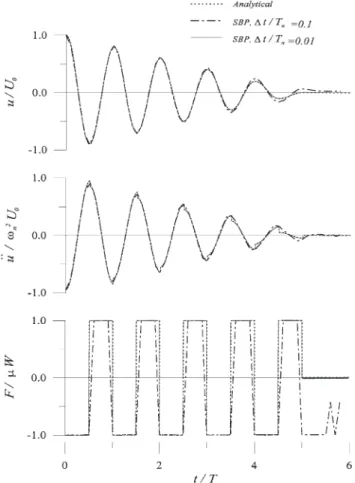
Fig. 2 illustrates the free vibration responses, in terms of displacement, acceleration and friction force, for

U0w 2

n/2mg=10 , considering the sampling ratio, ⌬t/Tn, of

0.1 and 0.01, respectively. For⌬t/Tn=0.1, significant

dis-crepancies exist between numerical (SBP) and analytical solutions, especially when the motion ceases after five cycles of free oscillation (as predicted by inequality (12)) where the estimated friction is seriously distorted. The error arises mainly from assuming a linear variation of the friction force between two consecutive sampling points in the analysis, an assumption which is not valid during stick–slip transitions or direction switches when both the acceleration and friction responses are discon-tinuous. However, the error becomes insignificant as the sampling ratio, ⌬t/Tn, decreases to 0.01. Numerical

results closely match the analytical solutions even during

Fig. 2. Free vibration of the SDOF Coulomb-friction-damped system (w2

(5)

phase transitions. A sampling ratio of 0.01, which is comparatively large for nonlinear dynamic analysis, is considered sufficient.

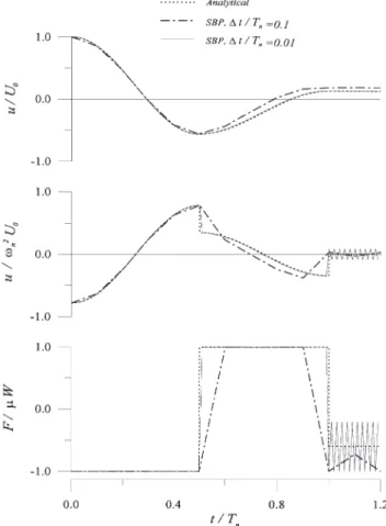
Fig. 3 further illustrates the corresponding results for

U0w2n/2mg=2.3. While the predicted displacement

response closely approximates the analytical displace-ment for ⌬t/Tn=0.01, acceleration and friction are only

accurate during the sliding phase. In the stick phase, fol-lowing one cycle of free oscillation, the numerical pre-diction does not converge to the analytical solution, even with a reduced sampling ratio. Nevertheless, the numeri-cal solution is not divergent either, indicating no error accumulation.

4.2. Harmonic response of a 2DOF sliding system

The response of sliding structures to harmonic support motion, studied by Mostaghel et al. [5] via a semi-ana-lytical procedure, is further investigated herein. Fig. 4 shows a single-story structure of mass m, damping c and stiffness k, supported by a foundation raft of mass M that can slide horizontally. The Coulomb frictional coef-ficient is m. When the ground moves with acceleration

x¨0, the dynamic response of the system is governed by

Fig. 3. Free vibration of the SDOF Coulomb-friction-damped system (w2

nU0/2mg=2.3).

Fig. 4. Single-story structure on sliding support.

冋

m m m M+m

册冉

x¨0=A sin⍀t with an excitation period of Tg=2p/⍀=0.5 s

and duration of excitation of 5 s. Response spectra for the absolute accelerations and sliding displacements nor-malized with respect to the peak ground acceleration, A, and the steady-state peak ground displacement,

D=A/⍀2_{, are obtained for coefficients of friction}

m=0.05, 0.10, 0.15, 0.20, for excitation amplitudes

A=0.5 g, and for mass ratios a=0.25, 0.50. The damping

ratio is assumed to be 5% of the critical damping, while all calculations use an integration step size of 0.005 s.

Figs. 5(a) and 6(a) show, respectively, the normalized spectral acceleration of structures with mass ratios a=0.25 and 0.5. The responses of the isolated structures are smaller than those of fixed-base structures.

(6)

Mean-Fig. 5. (a) Variations of acceleration with frequency ratio; (b) vari-ations of sliding displacement with frequency ratio (x=5%, a=0.25, A=0.5g, Tg=0.5 s).

while, the responses decrease with declining frictional coefficient. Figs. 5(b) and 6(b) illustrate, respectively, the normalized spectral displacement of sliding for mass ratios a=0.25 and 0.5. The structure slides further with a smaller frictional coefficient. Additionally, the spectral displacements do not vary significantly with frequency ratio when a=0.25. As the mass ratio increases to a=0.5, the spectral displacements become somewhat fre-quency dependent. Excellent agreement has been observed between the numerical results and the analyti-cal solution by Mostaghel et al., further confirming the effectiveness of the proposed numerical procedure.

4.3. Earthquake response of a five-story base-isolated structure

Finally, the earthquake response analysis of a proto-type five-story building implemented with friction pen-dulum seismic isolation bearings (FPS) is investigated using both the presented SBP method and the corrective pseudo-force iterative procedure (CPIP) by Nagarajaiah et al. [8].

In the CPIP method, the friction force is further rep-resented by Wen’s model [9] as

Fig. 6. (a) Variations of acceleration with frequency ratio; (b) vari-ations of sliding displacement with frequency ratio (x=5%, a=0.5, A=0.5g, Tg=0.5 s).

F⫽mWq (16)

where m is the friction coefficient, W is the weight of the structure and q is governed by a nonlinear differential equation as q˙⫽hx˙s⫺b兩x˙s兩兩q兩 n−1_q_⫺gx˙ s兩q兩 n (17) where h, b, g and n are parameters characterizing the hysteresis loops of the friction. To facilitate analysis, these parameters must be carefully calibrated for a pre-scribed hysteresis obtained by a component test of the isolation bearing. The friction mechanism of Mokha depicted by Eq. (2) is adopted with mmax=0.05,

mmin=0.036 and a=78.7 s/m (2 s/in) assumed in this

example.

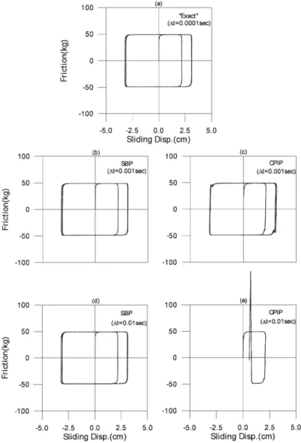
With no analytical solution available, the “exact” hys-teresis of a sliding bearing subjected to a harmonic exci-tation of 0.5 Hz for 30 s is illustrated in Fig. 7(a), which was simulated by the SBP method with⌬t=0.0001 s fol-lowing Mokha’s friction mechanism. Employing the SBP method with ⌬t=0.001 s, prediction of the hyster-esis is perfect (Fig. 7(b)), while the calculation is 107 times faster than that required by the “exact” solution in CPU time. When the step size further increases to 0.01

(7)

Fig. 7. Hysteresis of friction force under harmonic motion.

s, correlation of the result with the “exact” one is still excellent (Fig. 7(d)), while the calculation is 8369 times faster than that required by the “exact” solution. On the other hand, the parameters of Wen’s model in Eq. (17) are determined from a preliminary parametric study to be h=30, b=15, g=15, and n=2. Employing the CPIP method with ⌬t=0.001 s, the simulated hysteresis approximates the “exact” one closely, except at the cor-ners where reversing of sliding occurs (Fig. 7(c)), and the calculation is 89 times faster than that required by the “exact” solution. However, the numerical solution diverges when the step size further increases to 0.01 s (Fig. 7(d)).

The seismic response of a five-story model structure with FPS isolators is examined next. The radius of cur-vature of the FPS bearing is 1 m so that the vibration period of the isolated structure during sliding is shifted to 2 s. The system parameters of the structure are

sum-marized in Appendix B. The 1940 El Centro earthquake is used as the excitation.

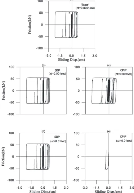
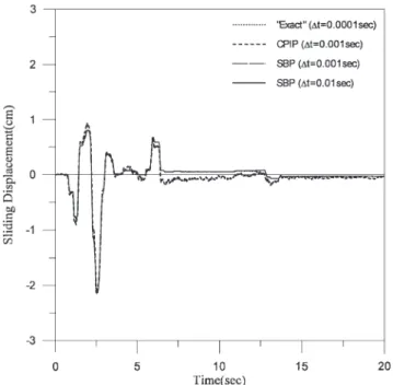
Fig. 8 illustrates the hysteresis of friction force. The “exact” solution in Fig. 8(a) is obtained by employing the SBP method with⌬t=0.0001 s, since there is no ana-lytical solution available. The results in Fig. 8(b,d) indi-cate the SPB method with ⌬t=0.001 or even 0.01 s can sufficiently predict the “exact” hysteresis. Employing the CPIP method, with the same parameters of Wen’s model calibrated in the harmonic case, the prediction of the hysteresis with ⌬t=0.001 s correlates well with the “exact” solution with only small discrepancies (Fig. 8(c)). However, the numerical result diverges when ⌬t=0.01 s. Fig. 9 illustrates the time history of the sliding displacement. The residual displacement after the earth-quake episode is found to be insignificant, indicating a good restoring capability of the FPS isolation system. Clearly, the results by the SBP method with ⌬t=0.001

(8)

Fig. 8. Hysteresis of friction force under the El Centro earthquake.

and 0.01 s coincide with the “exact” solution, while that by the CPIP with ⌬t=0.001 s deviates slightly from the “exact” solution. The responses of the roof displacement (relative to the base) reveal a similar trend, as depicted in Fig. 10. Besides, for an acceptable numerical accu-racy, the computational time required by the SBP method with⌬t=0.01 s is approximately 94 times faster than that required by the CPIP method with⌬t=0.001 s, without counting the time needed to calibrate Wen’s model. Furthermore, the structural response amplitude, illustrated in Fig. 11, is substantially reduced compared with that without seismic isolation (fixed), confirming the effectiveness of FPS isolation bearings under the El Centro earthquake.

5. Conclusions

This study has developed a numerical procedure based on a state-space difference equation and the concept of shear balance, with additional conditions of equilibrium and kinematic compatibility at the sliding interfaces for the dynamic analysis of sliding structures. Effectiveness of the algorithm is verified through examples of sliding systems, under conditions of either free vibration or har-monic excitations, for which analytical solutions are available. The proposed scheme accurately predicts the nonlinear behavior for forced vibration cases and free vibration cases with U0w2n/2mg being an integer.

How-ever, for free vibration cases with U0w 2

n/2mg being a

(9)

Fig. 9. Sliding displacement of the isolated structure under the El Centro earthquake.

Fig. 10. Roof relative displacement under the El Centro earthquake.

accurate during the sliding phases. Both the proposed scheme and a corrective pseudo-force iterative procedure are applied comparatively for seismic response analysis of a FPS-supported five-story building. Logically simple and easy to implement, the proposed scheme substan-tially simplifies the task with accuracy and efficiency enhanced to a large extent. The proposed scheme has the following features:

1. The dynamics of the sliding system is represented by

Fig. 11. Roof displacement with and without seismic isolation.

a single set of state-space equations without changing any system parameter during the analysis, regardless of either the slip or stick phase.

2. No prescribed hysteresis of friction force is needed, as required by the corrective pseudo-force iterative procedure. The friction force (or Lagrange multiplier) can be obtained by simple matrix algebraic calcu-lation.

3. A constant and relatively larger integration interval is allowed throughout the analysis, compared with the CPIP method. The numerical results that employ the proposed SBP method converge to the “exact” sol-utions with a step size as large as 0.01 s, thus helping to significantly reduce the computational effort. 4. It requires only a one-step correction without iteration

when the Coulomb’s model is considered as the fric-tion mechanism. With a moderate modificafric-tion, the numerical scheme can further resolve problems involving a more sophisticated frictional mechanism such as the Mokha’s model.

5. With the friction force(s) treated as an independent variable (vector), this algorithm is flexible enough to be extended further for solving dynamic problems of sliding structures with unsynchronized multiple sup-port motions.

Acknowledgements

This research is sponsored by the National Science Council of the Republic of China under grant no. NSC 88-2625-2009-001. The authors would also like to thank

(10)

Dr L.L. Chung, National Center for Research on Earth-quake Engineering, Taiwan, for his valuable discussions.

Appendix A

Without a loss of generality, a SDOF structure is con-sidered to investigate the numerical accuracy for both the Newmark and SSP methods.

A.1. Newmark method

The basic equations of the Newmark method are gen-erally formulated as mx¨[k]⫹cx˙[k]⫹kx[k]⫽⫺mw[k] (A1) x[k]⫽x[k⫺1]⫹⌬tx˙[k⫺1]⫹⌬t2

冋冉

1 2⫺a

冊

x¨[k⫺1] (A2) ⫹ax¨[k]

册

x˙[k]⫽x˙[k⫺1]⫹⌬t[(1⫺d)x¨[k⫺1]⫹dx˙[k]] (A3) where x[k] is the displacement at the kth time instant,

m, c and k are, respectively, the mass, damping and

stiff-ness of the system, w is the ground excitation, ⌬t is the integration time interval,a and d are parameters charac-terizing the approximation strategy. If dⱖ1/2 and aⱖ d/2, the Newmark method is unconditionally stable.

Eqs. (A1)–(A3) can be concisely expressed in a recur-sive matrix form as

Fig. A1. Frequency response function by the Newmark method (d=1/2, a=1/4, x=0.01). z[k]⫽Az[k⫺1]⫹Ew[k] (A4) where z[k]⫽

冤

x[k] x˙[k] x¨[k]

冥

冊

k mˆ

冥

is a 3×3 effective system matrix,

E⫽

冤

−⌬t2_am mˆ −⌬tdm mˆ −m mˆ

冥

is a 3×1 effective load vector, and mˆ=m+⌬tdc+⌬t2_{ak is}

the effective mass.

Taking a z-transformation of the difference equation

(11)

Eq. (A4), the structural response z[k] and the external disturbance w[k] are related in frequency-domain by

Z(z)⫽H(z)W(z) (A5)

where Z(z) and W(z) are the z-transforms of z[k] and

w[k], respectively. H(z)=(I⫺z−1A)−1E is the 3×1

fre-quency response function by assigning z=ej2pf⌬t_{. The}

dis-placement frequency response function, X(f), can be specifically calculated as

X(f)⫽D(I⫺e−j2pf⌬tA)−1E (A6)

where D=[1 0 0] is the location vector of the displace-ment.

A.2. State-space procedure (SSP)

The discrete-time state-space equation of a SDOF structure subjected to ground excitation can be expressed as

z[k]⫽Az[k⫺1]⫹E0w[k⫺1]⫹E1w[k] (A7)

where A=eA∗⌬t _{is a 2}_{×2 discrete-time system matrix,}

in which

Table 1

System parameter Parameter value

Mass matrix M (N s2_/m)

Stiffness matrix K (N/m)

Damping matrix C (N s/m)

Modal frequency before isolated f (Hz) [0.86 2.89 5.76 9.41 12.79]T

Modal damping factor before isolatedx (%) [3.00 3.00 3.00 4.90 6.66]T

Modal frequency after isolated f (Hz) [0.45 1.58 3.51 6.42 10.05 13.14]T

Modal damping factor after isolatedx (%) [0.33 4.10 3.96 3.67 3.58 6.90]T A∗⫽

冤

0 1 −k m − c m

冥

E0 is a 2×1 load matrix of the previous time-step, and

E1 is a 2×1 load matrix of the current time-step. The

SSP method is uncondionally stable if the structure itself is stable (that is, wn⬎0 and x⬎0), regardless of the

step size.

Taking a z-transform of the difference equation (A7), the structural responses z[k] and the external disturbance

w[k] are related in the frequency-domain by

Z(z)⫽H(z)W(z) (A8)

where Z(z) and W(z) are the z-transforms of z[k] and

w[k], respectively.

H(z)⫽(I⫺z−1A)−1(z−1E0⫹E1)

is the 2×1 frequency response function by assigning

z=ej2pf⌬t_{. The displacement frequency response function,}

(12)

X(f)⫽D(I⫺e−j2pf⌬tA)−1(e−j2pf⌬tE0⫹E1) (A9)

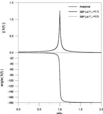
where D=[1 0] is the location vector of the displacement. By employing the Newmark method with d=1/2 and a=1/4, the displacement frequency response functions for ⌬t/Tn=0.1 and 0.2 are depicted in Fig. A1, while the

analytical solution is comparatively presented. When ⌬t/Tn=0.1, the peak of the frequency response is slightly

reduced in magnitude and shifted leftward, implying a distortion on the dynamic characteristics of the system. In addition, the peak shifts further as ⌬t/Tnincreases to

0.2. However, the SSP method indicates no distortion on the frequency response function, even if ⌬t/Tn=0.2, as

demonstrated in Fig. A2. This observation confirms a complete conservation of the structure’s dynamic characteristics employing the SSP method.

Appendix B. Parameters of a multi-story sliding structure

Table 1

References

[1] Buckle IG, Mayes RL. Seismic isolation history: application and performance — a world review. Earthquake Spectra 1990;6:161–201.

[2] Zayas V, Low SS, Main SA. The FPS earthquake resisting sys-tem, experimental report. Report no. UCB/EERC-87/01, Earth-quake Engineering Research Center, University of California, Berkeley, CA, June 1987.

[3] Kawamura S, Kitazawa K, Hisano M, Nagashima I. Study of a sliding-type base isolation system–system composition and element properties. In: Proc. 9th WCEE; Tokyo-Kyoto, vol. V, 1988:735–40.

[4] Westermo B, Udwadia F. Periodic response of a sliding oscillator system to harmonic excitation. Earthquake Engng Struct Dyn 1983;11:135–46.

[5] Mostaghel N, Hejazi M, Tanbakuchi J. Response of sliding struc-tures to harmonic support motion. Earthquake Engng Struct Dyn 1983;11:355–66.

[6] Mostaghel N, Tanbakuchi J. Response of sliding structures to earthquake support motion. Earthquake Engng Struct Dyn 1983;11:729–48.

[7] Yang YB, Lee TY, Tsai LC. Response of multi-degree-of-free-dom structure with sliding supports. Earthquake Engng Struct Dyn 1990;19:739–52.

[8] Nagarajaiah S, Reinhorn AM, Constantinou MC. Nonlinear dynamic analysis of 3-D-base-isolated structures. J Struct Engng, ASCE 1990;117(7):2035–54.

[9] Sues RH, Mau ST, Wen YK. System identification of degrading hysteretic restoring forces. J Engng Mech, ASCE 1988;114(5):833–46.

[10] Rosenbrock HH. Some general implicit processes for the numeri-cal solution of differential equations. Comput J 1964;18(1):50– 64.

[11] Lopez-Almansa F, Barbat AH, Rodellar J. SSP algorithm for lin-ear and nonlinlin-ear dynamic response simulation. Int J Numerical Meth Engng 1988;26:2687–706.

[12] Mokha AS, Constantinou MC, Reinhorn AM. Teflon bearing in base isolation. I: Testing. J Struct Engng, ASCE 1990;116(2):438–54.

[13] Mokha AS, Constantinou MC, Reinhorn AM. Teflon bearing in base isolation. II: Modeling. J Struct Engng, ASCE 1990;116(2):455–74.

[14] Chopra AK. Dynamics of surfaces — theory and applications to earthquake engineering. Englewood Cliffs, NJ: Prentice-Hall, 1995.