主動式多攝影機視訊監控系統之研究

行政院國家科學委員會補助專題研究計畫

□成果報告

期中進度報告

主動式多攝影機視訊監控系統之研究

計畫類別：

個別型計畫 □ 整合型計畫

計畫編號：NSC 97-2221-E-009-132-MY3

執行期間：

97 年 8 月 1 日至 98 年 7 月 31 日

計畫主持人：王聖智

共同主持人：

計畫參與人員：

黃敬群、周節、林瑋國

成果報告類型(依經費核定清單規定繳交)：

精簡報告 □完整報告

本成果報告包括以下應繳交之附件：

□赴國外出差或研習心得報告一份

□赴大陸地區出差或研習心得報告一份

□出席國際學術會議心得報告及發表之論文各一份

□國際合作研究計畫國外研究報告書一份

處理方式：除產學合作研究計畫、提升產業技術及人才培育研究計畫、

列管計畫及下列情形者外，得立即公開查詢

□涉及專利或其他智慧財產權，□一年□二年後可公開查詢

執行單位：交通大學電子工程系

中 華 民 國

98 年 6 月 10 日

應用於視訊監控之運動物體追蹤技術研究

Visual Surveillance System with Multiple Active Cameras

計畫編號：NSC 97-2221-E-009-132-MY3 執行期限：97年8月1日至98年7月31日 主持人：王聖智 (交通大學電子工程系教授) 計畫參與人員：黃敬群、周節、林瑋國 (交通大學電子所研究生)

中文摘要

在本計畫中，我們提出一套有效率的多 攝影機監控系統，能夠同時偵測場景中多物 體，進行物體類別標記，以及建立物體於多攝 影機內對應關係。在我們的系統中，我們首先 將多台攝影機所獨自取得的物體偵測資訊整 合到一個事後機率分佈(posterior distribution)， 這個機率分佈代表不同的地平面上有人物站 立其上的機率數值。接著，根據此事後機率分 佈 的資訊 ，系 統得以 透過 粒子取 樣的 方法 (sample-based manner)，有效率的找出在場景 中 物體的 個數 以及這 些物 體於地 平面 的位 置，基本上這套粒子取樣的方法結合了馬可夫 鏈蒙地卡羅取樣(Markov Chain Monte Carlo) 以及平均位移(Mean-Shift) 分群法。下一步我 們將求得的場景資訊輸入一套貝士階層架構 (Bayesian hierarchical framework)，這套架構採 用了馬可夫網路(Markov network)模型來達成 多物體的類別標記以及物體於多攝影機內對 應關係。理論上而言，多物體的類別標記與對 應被當成一個最佳化的問題，利用三維場景資 訊，影像色彩資訊，以及個別攝影機的偵測結 果，我們得以尋求最佳的結果。我們的實驗結 果顯示，即便在嚴重遮蔽的情況下，系統仍然 可以得到正確的結果。 關鍵詞：影像標記、圖學模型、物體對應、馬 可夫鏈蒙地卡羅、平均位移分群法。

Abstract

In this project, we propose an efficient way to simultaneously label and map targets over a multi-camera surveillance system. In the system, we first fuse the detection results from multiple cameras into a posterior distribution. This distribution indicates the likelihood of having some moving targets on the ground plane. Based on the distribution, isolated targets, together with their 3-D positions, are identified in a sample-based manner, which combines Markov Chain Monte Carlo (MCMC), and Mean-Shift clustering. The induced 3-D scene information is further inputted into a 3-layer Bayesian hierarchical framework (BHF), which adopts a Markov network to deal with the object labeling and correspondence problems. In principle, labeling and correspondence are regarded as a unified optimal problem subject to 3-D scene prior, image color similarity, and detection results. The experiments show that accurate results can be gotten even under situations with severe occlusion.

Keywords: Image labeling, Graphical models, Object correspondence, Markov Chain Monte Carlo, Mean-Shift clustering

Recently, the computer vision technology for video surveillance applications has made tremendous progress. Those applications may be roughly classified into single-camera systems and multi-camera systems. For a single-camera system, object labeling is an essential step for advanced analysis, like behavior understanding. However, a 2-D image lacks the depth information and thus the detection of moving targets usually suffers from the occlusion problem. The occlusion problem makes it difficult to correctly label or segment connective targets. Moreover, a supervised setting of targets number is usually needed for labeling. Unfortunately, this information is usually not available in practical applications.

On the other hand, for a multi-camera system, object correspondence is crucial. The cross reference of multiple camera views may ease the occlusion problem and provide a more reliable way for object labeling. Up to now, many multi-camera correspondence algorithms have already been proposed. For example, Khan et al. [1] checked the overlapped fields of view between cameras. Whenever a moving object enters the overlapped region, the object correspondence across multi-camera views can be established. In [2], the authors proposed a principal axis based correspondence among multiple cameras for data fusion. In [3], Black and Ellis establish the correspondence by comparing the distance between the projected epipolar lines and the detected objects in each 2-D image. In [4], Utsumi proposed the adoption of intersection points, which are the intersections of the 3-D lines emitted from the 2-D segmented regions of different camera views, to map objects. Nevertheless, most of these methods

require the foreground region of each target is correctly extracted in each camera view. Surely, this cannot be easily achieved in an occlusion case. In [5], Mittal launched the correspondence of objects by matching segmented regions along epipolar lines in pairs of camera views. The corresponding mid-points are then projected onto the 3-D space to yield a 3-D probability distribution map for the description of people’s positions. Although this method can relax the limitation of isolated foreground region, it requires camera color calibration for region matching. In this project, the major focus is to propose a unified method to label and map targets over multiple cameras. The proposed method can systematically estimate the target number, tackle inter-target occlusions problem, and doesn’t require color calibration.

2. SYSTEM OVERVIEW

In this project, we proposed a two-step procedure – information fusion and Bayesian inference – for labeling and mapping targets, especially for walking people on the ground plane. The goal of information fusion is to fuse consistent 2-D detection results of multiple cameras and build the scene knowledge. Here, we formulate a posterior distribution, called target detection probability (TDP), as the fused message pool to indicate the likelihood of having a moving target at a continuous-valued ground location. Based on the TDP distribution, the scene knowledge can be identified in a probabilistic sample-based manner, which combines Markov Chain Monte Carlo (MCMC) sampler and Mean-Shift clustering. For the Bayesian inference step, our goal is to retrieve

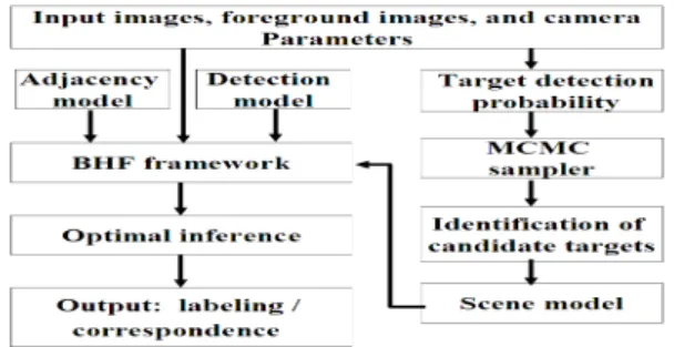
the optimal solution for labeling and correspondence. In our system, we regard labeling and correspondence as a unified optimal problem, subject to 3-D scene prior, image color similarity, and detection results. Note that the 3-D scene prior which represents the scene knowledge in Step one is defined as the scene model. The image color similarity is considered as the adjacency model, and the detection results are described in the detection model. Furthermore, by adopting the proposed Bayesian hierarchical framework (BHF) which models the optimal problem as a Markov network, we can infer the labeling and correspondence simultaneously in an efficient manner. In Fig. 1, we show the proposed system flow.

Fig. 1. System flow of the proposed algorithm.

3. INFORMATION FUSION

3.1. Target Detection Probability (TDP) distribution

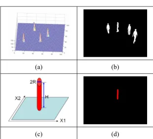
In the proposed system, we integrate the 2-D detection results of multiple cameras, which are the outputs of background subtraction based on Gaussian mixture model, by maintaining a target detection probability (TDP) distribution over time. This TDP distribution, as shown in Figure 2(a), expresses the probability of having a moving target at a ground location given a set of

foreground images from multiple cameras. In detail, we formulate the TDP as

1 1

( ) ( | ,..., _N) ~ ( ) ( ,..., _N| )

G X ≡p X F F p X p F F X

.

(1) In (1), X represents a location (x1, x2) on the ground plane. N is the number of static cameras in the multi-camera system. Fi denotes the foreground image (see Figure 2(b)) acquired from the ith camera view. Assume (m,n) denote the coordinates of a pixel on the foreground image, then ⎩ ⎨ ⎧ ∉ ∈ = regions foreground n) (m, if 0 regions foreground n) (m, if 1 ) , ( nm Fi

.

(2)

Moreover, given the location X, we assume the foreground images are conditionally independent of each other. Also, we assume p(X) is uniform distributed that indicates the equal possibility of finding a moving person at X. That is, we assume (1) can be written as

∏

= N i i N X p F X F F p X p 1 1,..., | )~ ( | ) ( ) (

.

(3)

On the other hand, to formulate p(Fi|X), we approximate a moving target at the ground position X as a cylinder like Figure 2(c). The height H and radius R of the cylinder are modeled as independent Gaussian random variables, with their priors p(H) and p(R) being pre-trained via training targets. Based on the pre-calibrated projection matrix of the ith camera and a sample pair (H, R), we project the cylinder onto the ith camera view to get the projected image Mi, as shown in Figure 2(d). Mathematically, we have

1 if (m,n) projected regions ( , |H,R,X) 0 if (m,n) projected regions i M m n _{= ⎨}⎧ ∈ ∉ ⎩ (4)

The expectation of the overlapped region of Mi and Fi with perspective normalization offers a reasonable estimate about p(Fi|X). That is, we define p(Fi|X) as

H,R

( | ) E ( )=_{i i i}(H,R,X)p(H)p(R)dHdR

p F X ≡ Ω

∫∫

Ω

,

(5)

where the normalized overlap correlation, Ωi, is defined as ( , ) ( , |H,R,X) (H,R,X) ( , |H,R,X) i i i i F m n M m n dmdn M m n dmdn Ω ≡

∫ ∫

∫ ∫

(a) (b) (c) (d)

Fig. 2. (a) The TDP of four moving targets. (b) A binary foreground image F. (c) A cylinder on the ground plane, with height H and radius R. (d) The cylinder's projection image M.

3.2. The extraction of scene knowledge

The 3-D scene knowledge required in our system includes: (a) the number of targets, (b) the likely position of each target, and (c) the unique ID of each target. In our method, the knowledge is extracted from the TDP distribution. Typically, the TDP distribution is composed of several clusters, with each cluster indicating a moving

target on the group plane. Hence, the detection of multiple moving targets can be treated as a clustering problem over the TDP distribution. Here, we adopt Markov Chain Monte Carlo (MCMC) sampler and Mean-Shift clustering to resolve the problem. The MCMC sampler is used to generate S samples {X0, X1, …, XS-1} from G(X) to stand for the TDP distribution. The Mean-shift clustering is used to cluster samples into different groups. Based on the clustered groups, we determine the number of moving targets, estimate the positions of each target, and assign a unique ID to each target. This mean-shift clustering method is efficient and robustness. It doesn’t require the prior knowledge about the number of targets. Moreover, in our system, we assign an unique ID for each sample X. Assume we have already identified T targets with the IDs {H1, H2, …, HT} on the ground plane. As the ID of the sample X is assigned to Hk, it means the target Hk may have an opportunity to appear at the location X. Based on these R samples {Xk,0, Xk,1, …, Xk,R-1} that belong to Hk, we can estimate the position distribution function p(X|Hk) for each target Hk. Here we model p(X|Hk) as a Gaussian function. The mean vector, the best estimate of the location of Hk, and covariance matrix of p(X|Hk) are estimated based on (6) and (7).

1 , 0 R k k j j X R µ − = =

∑

(6) 1 , , 0 ( )( ) R k k k T k j k j j X µ X µ R − = =

∑

− − C (7) 4. BAYESIAN INFERENCE

In our system, targets correspondence and image labeling are achieved by assigning a suitable ID from {H0, H1, H2, …, HT} to each pixel in N camera views, where T is the number of targets. Here, we introduce an extra ID “H0” to represent the “background” object. In principle, the best configuration of labels for one camera view depends on the image data, the 2-D detection result, and the information propagated from other cameras views. Here, we treat the TDP distribution as a scene knowledge pool collecting message from all cameras. Given the scene knowledge, we assume the ID labeling processes of different camera view are mutual independent. That is, we may label each camera view individually. Also, the target correspondence between different views is identified by matching the target ID in the labeling maps.

4.1. Bayesian hierarchical framework (BHF) The labeling process for one camera view is performed under the proposed Bayesian hierarchical framework, which is a 3-layer graphical model, as shown in Fig. 3. The top layer is a scene layer (SL), indicating the fused 3-D scene knowledge. The middle layer is a hidden labeling layer (HL), where each labeling node represents the ID of an image pixel. We define each labeling node hi in HL = {h1, ..,hM} to be one of the IDs in the set {H0, H1, H2, …, HT}. Note that Hk is the unique ID of target K. The bottom layer is a detection layer (DL), where each node di in DL = {d1, …,dM} indicates a detection result at the ith pixel with its value being either foreground (1) or background (0). M is the total number of pixels in the camera image. In BHF, we use the topological

inter-layer links and intra-layer links to incorporate three constraint models: the detection model, the adjacency model, and the scene model.

In mathematics, the BHF framework is a well defined undirected graphical model and reveals the statistical properties embedded in the labeling problem. Based on the graphical model theory, the joint probability distribution p(HL,DL,SL) over graphical nodes can be defined as the Boltzmann distribution in (8), where Z is the normalization constant and Ni is the neighbors of the ith pixel.

∑

∑

∑∑

∈ ∈ ∈ ∈ − − − M i iMjN j i A M i i i D L i S i h h E h d E S h E Zexp{ ( , ) ( , ) ( , )} 1 ₍₈₎

In (8), the definition of the clique energy functions, ES(hi,SL), ED(di,hi), and EA(hi,hj) are application oriented. In

Fig. 3. The BHF framework for pixel labeling in one image.

our system, they are defined by the scene model, the detection model, and the adjacency model, respectively.

The detection model ED(di,hi) used in (8) illustrates the correlation between the detection node di and the labeling node hi at the ith pixel. Ideally, we expect hi’s ID to be H0 if di is 0, and to be an element of {H1, H2, …, HT} if di is 1. Once the configuration violates this expectation, an empirically selected penalty constant α is

enabled to regularize the inference result. Hence, ED(di,hi) is defined as ))) ( , ( 1 ( ) , ( i i i i D d h d T h E ≡α× −δ , (9)

where δ(.) represents the Dirac’s delta function. In (9), T(hi) is set to 0 if hi is equal to H0; otherwise, T(hi) is set to 1.

The adjacency model EA(hi,hj) in (8) provides the smoothness constraints between two neighboring nodes hi and hi. Basically, neighboring labels tend to belong to the same ID. In our system, we softly force neighboring pixels to share the same label, especially when they have similar color appearance. We thus define EA(hi,hj) as (10) to reveal this property. In (10), Ii is the RBG color value at the ith pixel, and β is a pre-selected penalty constant.

(

)

( , ) min , (1 ( , ))/( )

A i j i j i j

E h h ≡ β β× −δ h h I I− (10)

To formulate ES(hi,SL), we first introduce the conditional probability p(hi|SL) which tells the probability of a label at ith pixel given the scene knowledge. Here, we build up a probability table for each pixel i. By using plentiful synthesized labeling images, the probability model is approximated by an accumulated histogram in a Monte Carlo manner. To generate the synthesized labeling images automatically, we stand T cylinders on the ground, indicating T moving targets. The height and radius of each cylinder are sampled from p(H) and p(R). The locations of T targets are sampled from p(X|Hk), where k is from 1 to T. With the camera projection parameters, a synthesized labeling image can be generated by projecting these T targets. Occasionally, more

than two targets may project onto the same image region and cause occlusion. The inter-occluded patterns and the order of depth can thus be determined by the distance from the camera’s 3-D location to the target’s mean location. Once if the probability p(hi|SL) is available, we define ES(hi,SL) as expressed in (11), which give a higher penalty value to a label hi with small p(hi|SL). )) | ( ln( ) , ( L i L i S h S ph S E ≡−

(11) 4.2. Optimal inference

With the joint probability distribution in (8), the ID labeling problem can be interpreted as an optimal inference process, as expressed in (12). Basically, we aim to find the most reasonable pixel labeling HL* with the detection layer (DL) set to the detection result (D), and the scene layer (SL) set to the current scene knowledge S.

(

)

(

)

* _{argmax[ln( ( , , ))]} ln( ( | )) 1 ( , ( )) argmax min 1,1 (1 ( , ))/( ) L L i L L L L H L i i i i M i M H i j i j i M j N H p D D H S S p h S d T h h h I I α δ β δ ∈ ∈ ∈ ∈ = = = ⎡ − − ⎤ ⎢ ⎥ = _{⎢ ⎥} − × − − ⎢ ⎥ ⎣ ⎦

∑

∑

∑∑

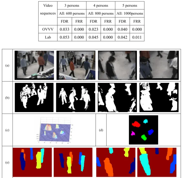
(12) To determine the optimal pixel labeling HL*, we adopt the graph-cut technique to derive the optimal inference of the undirected graphical model. In (12), α and β represent the trade-off among scene model, detection model, and adjacency model.

5. RESULTS AND CONCLUSIONS In our experiments, we set up four static cameras in our lab to capture real videos for testing. The snap shots of four camera views are shown in

Fig. 4(a). As we may find that there are severe inter-target occlusions among targets. In Fig. 4(b), we show the background subtraction results. Even though plentiful false alarms appear in the detection results, these errors cause little influence in the final multiple correspondence results. This is because the fusion step in the proposed algorithm collects only consistent information from all cameras and thus ignores the falsely detected parts which are inconsistent among cameras. Moreover, some detected foreground regions are connected together. This makes it very difficult to isolate individual targets by simply using the connected component analysis method. However, with the scene knowledge, the situation can be much relaxed. As shown in Fig. 4(c), the TDP still reveals a distinguishable distribution for target identification and localization. As shown in Fig. 4(d), the number and the location of the targets can be decided by mean-shift clustering. Finally, the results of labeling and corresponding are shown in Fig. 4(e). As expected, the scene knowledge is helpful in the labeling process, even under severe inter-target occlusion. To evaluate the proposed system in a quantitative way, we tested a few four-camera sequences with 3, 4, or 5 persons inside the scene. Each video sequence contains 200 frames and was either captured in our lab or synthesized by the ObjectVideo ○R _{Virtual Video (OVVV)}

environment. The false detection rate and false rejection rate of moving people are listed in Table 1. The whole system was implemented in a PC with a 2.0GHz Pentium-4 CPU. It takes about one second per time step for CIF color sequences. Especially for these three OVVV sequences, since their ground truth data are

available, we also calculate the deviation of the estimated locations with respect to the actual locations of the moving people. In our experiments, the mean deviations of true detection in these three sequences are only 0.061m, 0.060m, and 0.061m, respectively.

In summary, our algorithm is composed of two major steps: information fusion and Bayesian inference. Based on the proposed algorithm, two troublesome problems, inter-target occlusions and automatic determination of target number, can be handled in a systematic manner. Moreover, both object labeling and object correspondence can be achieved even under severe occlusion.

6. REFERENCES

[1] S. Khan and M. Shah, "Consistent labeling of tracked objects in multiple cameras with overlapping fields of view," IEEE Trans. Pattern Anal. Mach.

Intell., vol. 25, pp. 1355-1360, Oct. 2003.

[2] Weiming Hu, Min Hu, Xue Zhou, Tieniu Tan, Jianguang Lou and S. Maybank, "Principal axis-based correspondence between multiple cameras for people tracking," IEEE Trans. Pattern Anal. Mach. Intell., vol. 28, pp. 663-671, 2006.

[3] J. Black and T. Ellis, "Multi Camera Image Measurement and Correspondence," Measurement -

Journal of the International Measurement Confederation, vol. 35, pp. 61-71, July. 2002.

[4] A. Utsumi, H. Mori, J. Ohya and M. Yachida, "Multiple-human tracking using multiple cameras,"

IEEE International Conference on Automatic Face and Gesture Recognition, pp. 498-503, 1998.

[5]A. Mittal and L. Davis, “M2Tracker: A Multi-View Approach to Segmenting and Tracking People in a Cluttered Scene”, International Journal of Computer

Table. 1. False detection rate (FDR), false rejection rate (FRR).

3 persons 4 persons 5 persons

All: 600 persons All: 800 persons All: 1000persons Video sequences FDR FRR FDR FRR FDR FRR OVVV 0.033 0.000 0.023 0.000 0.040 0.000 Lab 0.053 0.000 0.045 0.000 0.042 0.011 (a)

(b)

(c) (d) (e)