台灣季節性消費品銷售預測之研究 - 政大學術集成

全文

(1)國立政治大學企業管理 MBA 學系碩士論文 MBA—Department of Business Administration National ChengChi University Master Thesis. 治政台灣季節性消費品銷售量預測之研究大立. ‧ 國. 學. Investigation on Forecasting Models for Predicting the Sales of Seasonal Consumer Products in Taiwan. y. 指導教授：張逸民博士. er. io. sit. Nat. Jason Pan. ‧. 潘家鋒. al. n. iv n C Advisor: Professor Ph.D. h e n gYegmingChang, chi U 中華民國 100 年 6 月 June 2011 國立政治大學碩士學位論文.

(2) ACKNOWLEDGEMENTS The completion of this dissertation would not have been possible without the assistance and guidance of several individuals who have contributed their valuable support in the preparation process of my research.. First and foremost, I would like to show my gratitude to my professor, Yegming Chang, whose encouragement and advice during the semester enabled me to think differently when. 治政大new insights, which have inspired approaching a new problem. He has provided me with many 立 me not only in a career aspect, but also in my personal development. ‧. ‧ 國. 學. I would also like to show my appreciation to all the professors who have given me lectures or. y. Nat. n. al. er. io. different ways.. sit. assistance during my studies at National ChengChi University. Many have enlightened me in. Ch. engchi. i n U. v. Last but not least, I would like to thank my family and friends for their genuine support. They were my motivation as I hurdled through all the obstacles on the path to the completion of my research.. i.

(3) ABSTRACT The trend seasonal demand pattern is encountered when both trend and seasonal influences are interactive. The problem of this research is to project the seasonal market sales using ice cream and fresh milk in Taiwan as examples. In order to improve the accuracy of forecast, two different methods are validated and the best forecasting method is selected based on the minimum Mean Square Error. In this study, we present two forecasting models used for evaluation to predict seasonal market sales of ice cream, fresh milk, and air conditioner in Taiwan. It includes Winters multiplicative seasonal trend model and the Decomposition method. Two different methods are validated and. 政治大. the best forecasting method is selected based on the minimum Mean Square Error.. 立. After the validation process, Winters multiplicative seasonal trend model is selected based on. ‧ 國. 學. the minimum MSE, and the monthly sales forecast for the year of 2011 is conducted using the data(60 months). Number Cruncher Statistical System (NCSS) is used for analyzing the data. ‧. which proves useful and powerful.. y. Nat. In summary, the results demonstrate that Winters multiplicative seasonal trend model has the. sit. smallest mean square error in this case. Therefore, we conclude that both Winters. al. er. io. multiplicative seasonal trend model and the Decomposition model are well fitted for. n. forecasting the seasonal market sales. Yet, Winters multiplicative seasonal trend model is the. Ch. i n U. v. better method to be used in this study since it generates the smallest mean square error (MSE) during the period of validation.. engchi. Key word: mean square error, Winters multiplicative seasonal trend model, Decomposition, seasonal trend demand. ii.

(4) TABLE OF CONTENTS ACKNOWLEDGEMENTS......................................................................................................... i ABSTRACT................................................................................................................................ ii TABLE OF CONTENTS........................................................................................................... iii TABLES ..................................................................................................................................... v FIGURES.................................................................................................................................. vii CHAPTER 1Introduction............................................................................................................ 1 1.1 Problem Statement......................................................................................................... 2 1.2 Research Objectives ...................................................................................................... 3. 政治大. 1.3 Research Data ................................................................................................................ 3. 立. 1.4 Organization of the Thesis............................................................................................. 4. ‧ 國. 學. CHAPTER 2Literature Review .................................................................................................. 5 CHAPTER 3Two Forecasting Models for the Seasonal Demand ............................................ 12. ‧. 3.1 Winters Multiplicative Trend Seasonal Model............................................................ 12. y. Nat. 3.2 Decomposition Forecasting ......................................................................................... 16. er. io. sit. 3.3 Estimation and Validation ........................................................................................... 21 3.4 Forecasting Accuracy .................................................................................................. 21. n. al. Ch. i n U. v. 3.5 Software used in the research ...................................................................................... 22. engchi. CHAPTER 4Data Collection and Analysis .............................................................................. 23 4.1 Data.............................................................................................................................. 23 4.2 Results of Forecasting for the Monthly Sales of Ice Cream........................................ 25 4.2.1 Validation .......................................................................................................... 25 4.2.2 Forecasts............................................................................................................ 34 4.3 Results of Forecasting for the Monthly Sales of Fresh Milk....................................... 37 4.3.1 Validation .......................................................................................................... 37 4.3.2 Forecasts............................................................................................................ 47 iii.

(5) 4.4 Results of Forecasting for the Monthly Sales of Air Conditioner............................... 51 4.4.1 Validation .......................................................................................................... 51 4.4.2 Forecasts............................................................................................................ 60 CHAPTER 5Conclusion, Implications, and Future Research .................................................. 65 5.1 Conclusions ................................................................................................................. 65 5.2 Implications ................................................................................................................. 66 5.3 Research Limitations ................................................................................................... 66 5.4 Future Research ........................................................................................................... 67. 政治大 Appendix A............................................................................................................................... 73 立 Appendix B ............................................................................................................................... 76 References................................................................................................................................. 69. ‧ 國. 學. Appendix C ............................................................................................................................... 80 Appendix D............................................................................................................................... 83. ‧. Appendix E ............................................................................................................................... 86. y. Nat. Appendix F................................................................................................................................ 91. sit. Appendix G............................................................................................................................... 94. n. al. er. io. Appendix H............................................................................................................................... 98. v. Appendix I .............................................................................................................................. 104. Ch. engchi. iv. i n U.

(6) TABLES Table 1: Monthly market sales report for ice cream and fresh milk in Taiwan........................ 23 Table 2: Summary of the values of the smoothing constants, α, β, γ, and the 14 coefficients for validation based on Winters Multiplicative Trend Seasonal Model (ice cream)...................... 26 Table 3: The monthly market sales for ice cream in Taiwan (forecasts vs. actual) for validation based on Winters Multiplicative Trend Seasonal Model.......................................................... 27 Table 4: Summary of the output report for validation based on the Decomposition Model (ice cream) ....................................................................................................................................... 29 Table 5: Seasonal component ratios for validation based on the Decomposition Model (ice cream) ....................................................................................................................................... 30 Table 6: The monthly sales forecast for ice cream in Taiwan (forecast vs. actual) for validation based on the Decomposition Model.......................................................................................... 31. 政治大 Table 7: MSE of forecast for validation based on Winters Multiplicative Trend Seasonal 立 Model (ice cream) ..................................................................................................................... 33. ‧ 國. 學. Table 8: MSE of Forecast for validation based on the Decomposition Model (ice cream)...... 33 Table 9: Summary of the values of the smoothing constants, α, β, γ, and the 14 coefficients for forecasting based on Winters Multiplicative Trend Seasonal Model (ice cream) .................... 34. ‧. Table 10: The monthly market sales for ice cream in Taiwan (forecast vs actual) based on Winters Multiplicative Trend Seasonal Model ......................................................................... 36. Nat. io. sit. y. Table 11: Summary of the values of the smoothing constants, α, β, γ, and the 14 coefficients for validation based on Winters Multiplicative Trend Seasonal Model (fresh milk) ............... 38. n. al. er. Table 12: The monthly market sales for fresh milk in Taiwan (Forecasts vs. Actual) for validation based on Winters Multiplicative Trend Seasonal Model......................................... 40. Ch. i n U. v. Table 13: Summary of the output report for validation based on the Decomposition Model (fresh milk)................................................................................................................................ 42. engchi. Table 14: Seasonal Component Ratios for validation based on the Decomposition Model (fresh milk)................................................................................................................................ 42 Table 15: The monthly sales forecast for fresh milk in Taiwan (forecast vs. actual) for validation based on the Decomposition Model......................................................................... 43 Table 16: MSE of Forecast for validation based on Winters Multiplicative Trend Seasonal Model (fresh milk) .................................................................................................................... 46 Table 17: MSE of Forecast for validation based on the Decomposition Model (fresh milk)... 47 Table 18: Summary of the values of the smoothing constants, α, β, γ, and the 14 coefficients for forecasting of fresh milk based on Winters Multiplicative Trend Seasonal Model............ 48 Table 19: The monthly market sales for fresh milk in Taiwan (Forecast vs Actual) based on Winters Multiplicative trend seasonal model ........................................................................... 49 v.

(7) Table 20: Summary of the values of the smoothing constants, α, β, γ, and the 14 coefficients for validation based on Winters Multiplicative Trend Seasonal Model (air conditioner) ........ 52 Table 21: The monthly market sales for air conditioner in Taiwan (forecasts vs. actual) for validation based on Winters Multiplicative Trend Seasonal Model......................................... 53 Table 22: Summary of the output report for validation based on the Decomposition Model (air conditioner) ............................................................................................................................... 55 Table 23: Seasonal component ratios for validation based on the Decomposition Model (air conditioner) ............................................................................................................................... 56 Table 24: The monthly sales forecast for air conditioner in Taiwan (forecast vs. actual) for validation based on the Decomposition Model......................................................................... 57 Table 25: MSE of forecast for validation based on Winters Multiplicative Trend Seasonal Model (air conditioner) ............................................................................................................. 59. 政治大. Table 26: MSE of Forecast for validation based on the Decomposition Model (air conditioner) ................................................................................................................................................... 60. 立. Table 27: Summary of the values of the smoothing constants, α, β, γ, and the 14 coefficients for forecasting based on Winters Multiplicative Trend Seasonal Model (air conditioner) ...... 61. ‧ 國. 學. Table 28: The monthly market sales for air conditioner in Taiwan (forecast vs actual) based on Winters Multiplicative Trend Seasonal Model ......................................................................... 62. ‧. n. er. io. sit. y. Nat. al. Ch. engchi. vi. i n U. v.

(8) FIGURES Figure 1: Methodology tree for forecasting (Forecastingprinciples.com) .................................. 6 Figure 2: The monthly market sales and forecasts for ice cream in Taiwan(ton) for validation based on Winters Multiplicative Trend Seasonal Model.......................................................... 27 Figure 3: The monthly market sales and forecasts for ice cream in Taiwan(ton) for validation based on the Decomposition Model.......................................................................................... 31 Figure 4: The monthly market sales forecast for ice cream in Taiwan(ton) based on Winters Multiplicative Trend Seasonal Model....................................................................................... 35 Figure 5: The monthly sales and forecasts for fresh milk in Taiwan(ton) for validation based on Winters Multiplicative Trend Seasonal Model. ................................................................... 39 Figure 6: The monthly market sales and forecasts for fresh milk in Taiwan(ton) for validation based on the Decomposition Model.......................................................................................... 43. 政治大 Figure 7: The monthly market sales forecast for fresh milk in Taiwan(ton) based on Winters 立Model....................................................................................... 49 Multiplicative Trend Seasonal. ‧ 國. 學. Figure 8: The monthly market sales and forecasts for air conditioner in Taiwan(ton) for validation based on Winters Multiplicative Trend Seasonal Model......................................... 53. ‧. Figure 9: The monthly market sales and forecasts for air conditioner in Taiwan(ton) for validation based on the Decomposition Model......................................................................... 57. n. al. er. io. sit. y. Nat. Figure 10: The monthly market sales forecast for air conditioner in Taiwan(ton) based on Winters Multiplicative Trend Seasonal Model ......................................................................... 62. Ch. engchi. vii. i n U. v.

(9) CHAPTER 1 Introduction In today’s business, management is challenged with rapid changes and competitive environments. Forecasting product demand with trend and seasonality is very important to any company including supplier, manufacturer, and retailer. Market demands of most products remain uncertain until the selling season begins. In many cases, trend and seasonality are important features for company’s products. Trends may stem. 政治大. from changes in social environment, technological environment, economical environment,. 立. political environment, market conditions, or other industrial competition. Business cycles. ‧ 國. 學. include the recurrent patterns of prosperity, warning, recession, depression, and recovery. Many products have seasonal effects. For example, the life cycles of these seasonal products are short and the demands are uncertain. For instance, the demand for ice cream, fresh milk,. ‧. electricity, air condition equipment, winter apparel, fashion goods, Christmas gifts are higher. y. Nat. during specific seasons and hold seasonality, trends, or cyclic demand patterns. Moreover,. sit. future market sales of these seasonal products may not follow the historical pattern of past. er. io. demand, which may imply different predictions at different time periods. Therefore, market. al. iv n C effective manager. The most popularhforecasting techniques e n g c h i U currently available are based on extrapolation of historical market sales data. For accurate forecasting, it is important to n. sales planning for seasonal and short life-cycle products are considered a vital task for an. estimate the parameters of forecasting models with the most recent market sales information and forecast can then be updated as new market sales information becomes available. The high levels of customer service and efficient operations come from accurate demand forecasts, while inaccurate forecasts tend to lead to poor levels of customer satisfaction and higher cost operations. One of the first steps a business can take to improve its efficiency and effectiveness is to improve the quality of the market sales forecasts. Over a hundred NT a scoop, the high-price premium quality ice cream in Taiwan has already become a very popular and common consumer good. At first there was the monopolistic ice 1.

(10) cream brand Haagen-Dazs, then came the addition of Movenpick. In the year of 2007, Unipresident’s Convenience Store subsidiary 7-ELEVEN had obtained the authorization of Cold Stone and opened its first franchise store in Taiwan. As of January, 2011, there are 28 Cold Stone ice cream stores in Taiwan. In the past, there had been very little market sales forecast-related research on ice cream in Taiwan. One sunny day in the summer of 2010, as I was enjoying the melting cream in my mouth, cotton-candy flavored ice cream that was scooped into a cookie-made bowl at Cold Stone, it had occurred to me, got me thinking and wondering about what the demand of ice cream is like in Taiwan. The demand of ice cream obviously follows a seasonal trend, but how. 政治大. can we more accurately project the sales of ice cream in Taiwan to prevent from overproduction or importation of ice cream-related products, since the ice cream market had. 立. changed over the past five years or even before that. As consumers are more and more willing. ‧ 國. 學. to pay over a hundred NT a scoop for premium quality ice cream, more popular and bigger brands had entered to compete in Taiwan, including Haagen-Dazs, Movenpick, Cold Stone,. ‧. etc. And that was when I thought that it would be a good topic to do study and research on for my thesis. Fresh milk also possesses a pattern of trend and seasonality. And it is a necessity to. y. Nat. each family. The demand of fresh milk is strong in summer and slow in winter. Both ice cream. io. sit. and fresh milk are categorized as consumer products. Because of the similarity, their demand. n. al. er. data are selected for the research. In addition, air conditioner is another seasonal consumer product that is selected for comparison.. Ch. engchi. i n U. v. Little research hadinvestigated on the comparison of the Winters Model and the Decomposition Model to forecast the market sales of seasonal products in Taiwan, such as ice cream, fresh milk, and air conditioner. Therefore, it initiates the motive of this research.. 1.1 Problem Statement 2.

(11) The trend seasonal demand pattern is encountered when both trend and seasonal influences are interactive. The problem of this research is to project the seasonal market sales using ice cream,fresh milk, and air conditioner in Taiwan as examples. In order to improve the accuracy of forecast, two different methods are validated and the best forecasting method is selected based on the minimum Mean Square Error.. 1.2 Research Objectives The goal of this study is to project the market sales of a seasonal product such as ice cream,. 政治大. fresh milk, and air conditioner. Winters multiplicative seasonal trend model and the Decomposition method will be discussed and evaluated. In order to gain forecast accuracy, we. 立. will compare these two forecasting models and adopt the best forecasting technique through. ‧ 國. 學. the validation procedure based on the minimum Mean Squared Error (MSE). The improvement in market sales forecast offers an organization with potential cost reductions,. ‧. profit increase, operations improvement, and assists top managers to formulate some competitive strategies.. n. al. er. io. sit. y. Nat 1.3 Research Data. Ch. i n U. v. The dataset used in the research for ice cream and milk was obtained from the Monthly Report. engchi. of Industrial Production in Taiwan through the Department of Statistics, Ministry of Economic Affairs, ROC. The dataset for air conditioner was obtained from the Industrial Raw Material Price and Volume Information Database. The datasets represents the partial market demand of ice cream, fresh milk, and air conditioner in Taiwan over a time period from January 2006 to December 2010(60 months). The monthly demand from January 2006 to December 2009(48 months) is used to estimate the parameters of the forecasting models and validate the forecasts for the period from January 2010 to December 2010(12 months). Through validation process, a good model is determined and forecasts are performed for the period from January 2011 to December 2011(12 months). 3.

(12) 1.4 Organization of the Thesis This thesis is organized into five chapters. Chapter 1 is the introduction of this paper. Chapter 2 presents the literature review and some comments. Chapter 3 describes and discusses the models in this study. Chapter 4 covers data analysis and finds. Finally, Chapter 5 summarizes conclusions, implications, and future research.. 立. 政治大. ‧. ‧ 國. 學. n. er. io. sit. y. Nat. al. Ch. engchi. 4. i n U. v.

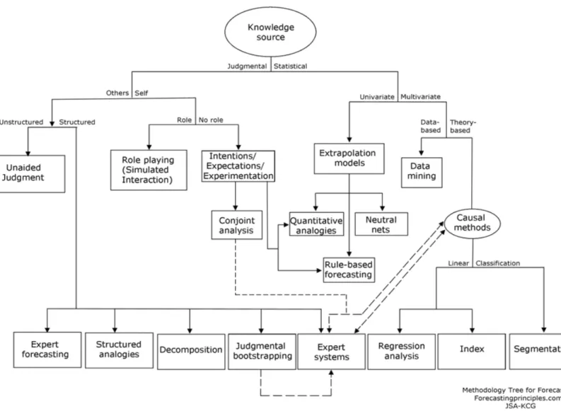
(13) CHAPTER 2 Literature Review Forecasting techniques have been discussed and classified by researchers (Small,1980; Georgoff and Murdick, 1986; Rao and Cox, 1987; Bails, Peppers, 1993; Bolt, 1994; Mentzer and Kahn, 1995; Peterson and Lewis, 1999; Cox and Loomis, 2001).Johnston and Marshall (2003) summarized some advantages and limitations of the various forecasting methods. Scott Armstrong (2001) developed one hundred and thirty-nine principles for forecasting, which include defining a problem, collecting information about it, selecting and applying. 政治大 nine generalizations that can improve forecast accuracy. In his article, Scott Armstrong 立 suggested on how to formulate a forecasting problem, how to tap managers’ knowledge, and methods, evaluating methods, and deriving forecasts. Later, Armstrong (2005) summarized. ‧ 國. 學. how to select appropriate forecasting methods.. Furthermore, Armstrong (2010) developed a very useful Methodology Tree (see Figure 1) for. ‧. forecasting which classifies all possible types of forecasting methods into categories and. sit. y. Nat. shows how they relate to one another.. io. er. The content of the Methodology Tree are summarized as follows:. al. iv n C relationships between a variable to be explanatory variables. hforecast e n gand chi U n. Causal models: Theory, prior research and expert domain knowledge are used to specify. Classification: If the problem is composed of groups that act in different ways in response to a change, one can study each group separately, then add across segments. Conjoint analysis: Elicit preferences from consumers for various offerings by using combinations of features. Regression-like analyses are then used to predict the most desirable design. Data-based: Experience and prior research are not available and so one must try to infer relationships from the data.. 5.

(14) Data mining: Letting the data speak for themselves. In general, theory is not considered. Despite its widespread use and many claims of accuracy, we have been unable to find evidence that data mining provides forecasts that are more accurate than those from alternative methods.. 立. 政治大. ‧. ‧ 國. 學. n. er. io. sit. y. Nat. al. Ch. engchi. i n U. v. Figure 1: Methodology tree for forecasting (Forecastingprinciples.com). Decomposition: Decomposition is a method for dealing with such problems by breaking down (decomposing) the estimation task down into a set of components that can be more readily estimated, and then combining the component estimates to produce a target estimate. 6.

(15) Expert Forecasting refers to forecasts obtained in a structured way from two or more experts. Expert systems: Rules for forecasting are derived from the reasoning experts use when making forecasts. Obtain knowledge from diverse sources such as surveys, interviews, protocol analysis, and research papers. Extrapolation: Use time-series data, or similar cross-sectional data, to predict. Index: In situations with many causal variables and few observations, the forecaster can nevertheless often use prior domain knowledge to assess the directional influence of individual variables on the outcome. The values of explanatory variables can be assessed subjectively,. 政治大. for example as zero or one, or can be normalized quantitative data where available. An index forecast is the sum of the values of the explanatory variables.. 立. Intentions/expectations/experimentation: Survey people about their intentions or. ‧ 國. 學. expectations regarding their future behavior or those of their organization. Analyze the survey data to derive forecasts. Conduct an experiment by changing key causal variables in a. ‧. systematic way such that the independent variables are not correlated with one another. Estimate relationships from responses to the changes and use these estimates to derive. y. Nat. sit. forecasts. Experiments can be used to predict the effects of different policies or regulatory. n. al. er. io. schemes, or to assess the effectiveness of alternative advertisements.. Ch. engchi. i n U. v. Judgmental: Available data are inadequate for quantitative analysis or qualitative information is likely to increase accuracy, relevance, or acceptability of forecasts. Judgmental bootstrapping: Derive a model from knowledge of experts’ forecasts and the factors they used to make their forecasts using regression analysis. Knowledge source: When reliable objective data are available, they should be used. Still, one might benefit from also using subjective methods. Linear: The problem can be modeled as linear in the parameters.. 7.

(16) Multivariate: Data are available on variables that might affect the behaviour of interest. No role: Roles are not expected to influence behavior, or knowledge about the roles is lacking, or there are many actors with different roles. Others: Knowledge exists about the expected behavior of other people or organizations. Quantitative analogies: Experts identify analogous situations for which time-series or crosssectional data are available, and rate the similarity of each analogy to the data-poor target situation. These inputs are used to derive a forecast. Regression analysis: Sometimes referred to as “econometric modeling”, forecasting using. 政治大. models with parameters estimated from historical data using statistical techniques is, however,. 立. widely relevant.. ‧ 國. 學. Role: People's roles influence their behaviors and there is knowledge about these roles. Role playing/Simulated interaction: In role playing, people are expected to think in ways. ‧. consistent with the role and situation described to them. If this involves interacting with people with different roles for the purpose of predicting the behavior of actual protagonists,. Nat. sit. y. we call it simulated interaction. That is, people act out prospective interactions in a realistic. er. io. manner. The role-players' decisions are used as forecasts of the actual decision.. al. n. iv n C using an expert system to extrapolatehtime series. Most U features are identified by e n g c h i series. Rule-based forecasting: Expert domain knowledge and statistical techniques are combined automated analysis, but experts identify some factors. In particular they identify the causal forces acting on trends. Segmentation: Where a heterogeneous whole can be divided into parts that act in different ways in response to changes, that are relatively homogenous, and that can be forecast more accurately than can the whole. Self: People have valid intentions or expectations about their behavior. Both are most useful when (1) responses can be obtained from a representative sample, (2) responses are based on good knowledge, (3) there are no reasons to lie, (4) new information is unlikely to change the 8.

(17) behavior. Intentions are more limited than expectations in that they are most useful when (5) the event is important, (6) the behavior is planned, and (7) the respondent can fulfill the plan (so, for example, the behavior is not dependent on the agreement of other people. Statistical: Relevant numerical data are available. Structured: Formal methods are used to analyze the information. This means that the rules for analysis are written in advance and they are rigorously adhered to. Records should be kept of how the procedures were administered. Structured analogies: An expert lists analogies to a target, describes similarities and. 政治大. differences, rates similarity, and matches each analogy's decision (or outcome) with a potential target situation decision (or outcome). The outcome implied by the top-rated analogy is used. 立. as a forecast.. ‧ 國. 學. Theory-based: Experience and prior research provide useful information about relationships relevant to the forecast.. ‧. Unaided judgment: Experts think about a situation and predict how people will behave. They. y. Nat. might have access to data and advice, but their forecasts are not aided by formal forecasting. sit. methods. This is the most commonly used method. It is fast, inexpensive when only a few. er. io. forecasts are needed, and can be used in cases where small changes are expected. It is most. al. n. iv n C (e.g., weather forecasting, betting onhsports, e n and h i Uin bridge games.) g cbidding. likely to be useful when the forecaster gets good feedback about the accuracy of his forecasts. Univariate :Historical data are available on the behaviour that is to be predicted. Unstructured: The information is used in an informal manner. Many researchers have investigated the classification criteria for forecasting methods such as Clemen(1989), McGuiganandMoyler (1989),BailsandPerpers (1993), Bolt (1994), Hall (1994),Taylor (1996), Kinnear, Reekie, and Crook (1998), Makridakis and Wheelwright(1998), Kennedy (1999), Peterson and Lewis (1999), Kirsten (2000), Goodwin (2002), LarrickandSoll (2006), Green and Armstrong (2007). 9.

(18) Decomposition is a method designed for solving this kind of problems by breaking down (decomposing) the forecasting task into a set of components that can be more readily estimated, and then combining the component estimates to produce a target estimate (Armstrong,2001). Persons (1919, 1923) started the research on decomposing a seasonal time series. Since then, many forecasters had devoted to developing forecasting methods to predict data time series with trend and seasonality. Those methods include Decomposition, Winters exponential smoothing, Time series regression, and ARIMA models (Bowerman and O’Connell, 1993; Hanke and Reitsch, 1995). Winters multiplicative seasonal trend model, one of the most popular forecasting models, was. 政治大. first developed by Charles C. Holt. Then, Peter R. Winters extended the model to forecast the seasonal demands. (Holt, 1957; Winters, 1960). Later, Box and Jenkins (1976) extended Holt-. 立. Winters model to the seasonal ARIMA model. The applications of ARIMA model are well. ‧ 國. 學. adopted by the industries. (Kurawarwala and Matsuo, 1998; Hyndman, 2004) Neural Networks (NN) models are also used for time series forecasting ( Hill, O’Connor and. ‧. Reus, 1996; Faraway and Chatfield,1998; Zhang et al., 1998; Nelson et al., 1999; Hansen and Nelson, 2003; Yamaha and Eurasia, 1991;A.N. Refenes,1993;White,1988; Kamijo and. y. Nat. er. io. and Fan,2009; Chang, et al.,2009; Chang, et al., 2009).. sit. Tanigawa,1990; Kimoto and Asakawa,1990; Schoeneburg, 1990; Hearing, 2006;Chang,Liu. al. n. iv n C Time Series Regression, ARIMA and models. In this empirical research, hNeural e n gNetworks chi U. Suhartono, et al. (2005) compare some forecasting methods including Decomposition, Winters, their focus is to study whether a complex method always give a better forecast than a simpler method. A real time series data of airline passenger was performed on these models. The findings show that the more complex model does not always yield a better result than a simpler one. Little research compared the forecasts of the market sales of seasonal products (such as ice cream, fresh milk, and air conditioner) in Taiwan, betweentheWinters Model and Decomposition Model. Therefore, it creates the motive of this research.. 10.

(19) This study tries to compare the performance of the Winters Model and the Decomposition Model for seasonal consumer products in Taiwan, using ice cream, fresh milk, and air conditioner as examples, to determine the better forecasting model. Through the validation process, the best method is to be selected based on the minimum Mean Square Error.. 立. 政治大. ‧. ‧ 國. 學. n. er. io. sit. y. Nat. al. Ch. engchi. 11. i n U. v.

(20) CHAPTER 3 Two Forecasting Models for the Seasonal Demand. Two forecasting models to predict seasonal market sales of ice cream, fresh milk, and air conditioner in Taiwan will be presented in this chapter—including theWinter’s multiplicative trend seasonal model and the Decomposition method. The two forecasting models are presented as follows.. 政治大. 3.1 Winters Multiplicative Trend Seasonal Model. 立. The method presented here is a slight modification by Nick T. Thomopoulos (1988) to Winters. ‧ 國. 學. (1960) original description .Seasonal Demand of a product follows a pattern that has both “trend” and “seasonal” influences. The trend is either increasing or decreasing at a steady rate, and the same for the seasonal influence as shown in the horizontal seasonal market sales. ‧. pattern. The two factors coupled together give a pattern where the seasonal changes are bigger. y. Nat. for the higher levels of the trend than for the lower. A forecasting technique that applies for. sit. this type of market sales pattern is the multiplicative trend seasonal model.. er. io. The multiplicative trend seasonal model is appropriate when the expected demand for a. al. iv n C is the seasonal ratio at time t . In h this ) defines the general trend of the epattern, n g c(ha i btU n. product or item is  t  (a  bt )  t . Here a is the intercept or level at t  0 , b is the slope, and. t. expected demand. This trend is influenced by the seasonal ratio  t to yield the specific. expected demand at time t . Again, when  t >1, then  t is larger than the trend, and when  t <1, then  t is below the trend. With this pattern the seasonal influence is larger when the trend is at a higher level than when it is at a lower level. The expected demand at time (t   ) is defined by.  t   (at  b )  t  where at is the level at time t , b is the slope, and  t  is the seasonal ratio at (t   ) . 12.

(21) The role of the forecasting model is to use the history of demands to estimate 14 unknown coefficients in the demand pattern. At the current time T, these estimates are. aˆ T for aT bˆT for b. and rT  for  T    1,2, ,12 Three smoothing parameters ( ,  , and  ) are used for this purpose, where each lie in the interval (0,1). Parameter  is a smoothing parameter for aˆ T ,  is used to find bˆT , and  is. 政治大 Two phases are followed in 立 applying the model. The first is the initialization phase, which uses. for rT  .. past demands to get the system started. The second is the updating phase, where the forecasts. ‧ 國. 學. are altered as each new market sales entry becomes available. Descriptions of each of these. ‧. Nat. Initialization. y. phases follow.. sit. The purpose of the initialization phase is to start the system off with good estimates of aT , b ,. n. al. er. io. and  T  (   1,2, ,12 ). These estimates are found through the use of the past market sales. i n U. v. entries that are available to the forecaster. The past sales are again conveniently grouped into. J years：. Ch. engchi. Year 1： x1 , x2 ,, x12 Year 2： x13 , x14 ,, x24  Year J： xT 11 , xT 10 ,, xT where J=. T 12. In order to carry out the initialization, the following nine steps are followed： 13.

(22) 1. Find the average monthly market sales for the first and last year(year J). These are x(1)  x( J ) . 1 ( x1    x12 ) 12. 1 ( xT 11    xT ) 12. 2. Estimate the slope using b0 . x ( J )  x (1) T  12. Note that the change from x (1) to x ( J ) takes place over (T  12) months. This is because. 政治大 is representative of t  T  5.5 . Hence, the time span separating these time 立. x (1) is the average of the first year and is representative of time period t  6.5 , and in a. like way x ( J ). ‧ 國. 學. periods is T  12 months.. 3. The deseasonalized level at t  0 is now estimated by. a0  x(1)  6.5b0. ‧. 4. Carrying forward this trend, the deseasonalized level at time t becomes. y. sit. Nat. a t  a 0  b0 t. io. n. al. Ch. x ~ rt  t t  1,2, , T at. engchi. er. 5. A seasonal ratio for each month is now found. For month t this is. i n U. v. 6. The seasonal ratio are grouped by calendar months to find the average for each such month, i.e., r1 . 1 ~ ~ (r1  r13    ~ rT 11 ) J. r2 . 1 ~ ~ ( r2  r14    ~ rT 10 ) J.  r12 . 1 ~ ~ (r12  r24    ~ rT ) J. 14.

(23) 7. The seasonal ratios (r1 ,, r12 ) are normalized so that their average value is 1. This is by r. r rˆt  t. 1 (r1    r12 ) 12. r. for t  1,2,  ,12. 8. Starting at t  1 and continuing until t  T , the following three recursive relations are carried forward：. aˆ t   (. xt )  (1   )(aˆ t 1  bˆt 1 ) rˆt. bˆt   (aˆ t  aˆ t 1 )  (1   )bˆt 1. 立. 治政 x rˆ   ( )  (1  大 )rˆ t. t 12. t. aˆ t. Nat. rT  . 1 ( rˆT 1    rˆT 12 ) 12 1 rˆT  for   1,2, ,12 r. y. r. sit. average is 1. This step is performed as follows：. ‧. ‧ 國. 學. 9. The 12 most current estimates of the seasonal ratios are now normalized so that their. er. io. Having performed the preceding nine steps, the initialization process is complete. The estimates that are carried forward are aˆ T , bˆT , and rT 1 , rT  2 , , rT 12 . These may also be. al. n. iv n C used to generate forecasts as of t  T . The forecastUfor the  th future time period is hengchi xˆ ( )  (aˆ  bˆ )r T. T. T. T . Note that a seasonal ratio is estimated for each of the 12 calendar months. In this way rT 13  rT 1. rT 14  rT  2 . rT  24  rT 12 can be used should forecasts be required for   12 . 15.

(24) Updating With each passing time period, a new market sales entry becomes available and is used to update the 14 coefficients. Again using xT as the current demand, then. aˆT   (. xT )  (1   )(aˆT 1  bˆT 1 ) rT. bˆT   ( aˆ T  aˆ T 1 )  (1   )bˆT 1. rT 12   (. xT )  (1   )rT aˆ T. Now rT 1 to rT 12 are normalized so that their average is 1.. 政治ˆ 大 xˆ ( )  (aˆ  b  )r. The updated forecasts are generated at this time. For the  th future time period, the forecast is. 立. T. T. T. T . As before, should  exceed 12, the seasonal ratios are repeated. For example, rT 13  rT 1 ,. ‧ 國. 學. rT 14  rT  2 , and so forth.. ‧. 3.2 Decomposition Forecasting. y. Nat. sit. Decomposition is a method for dealing with forecast problems by breaking down. er. io. (decomposing) the estimation task down into a set of components that can be more readily. al. iv n time series decomposition series U i into five components: mean, trend, ea ntime h c g seasonality, cycle, and randomness. Makridakis (1998) expressed decomposition model as n. estimated, and then combining the component estimates to produce a target estimate. Classical. Ch separates. Value=(Mean)x (Trend)x (Seasonality)x (Cycle)x (Random) Note that this model is multiplicative rather than additive. Although additive models are more popular in other areas of statistics, forecasters have found that the multiplicative model fits a wider range of forecasting situations. Decomposition is often used by forecasters for it is easy to understand (and to explain to others). Complex ARIMA models are popular among statisticians. However, they are not as well-accepted among forecasting practitioners. For seasonal (monthly, weekly, or quarterly) 16.

(25) data, decomposition methods are often as accurate as the ARIMA methods and they provide additional information about the trend and cycle, which may not be available in ARIMA methods. Decomposition has one disadvantage: the cycle component must be input by the forecaster since it is not estimated by the algorithm. This may be avoided by ignoring the cycle, or by assuming a constant value. Some forecasters consider this a strength, because it allows the forecaster to enter information about the current business cycle into the forecast. Decomposition Method. 政治大 Xt =UTtCtS tRt. The basic decomposition method consists of estimating the five components of the model. n. al. St. denotesseason.. Rt. denotesrandomerror.. t. denotesthetime period.. Ch. y. sit. denotescycle.. io. Ct. denotesthelineartrend.. Nat. Tt. denotesthemeanoftheseries.. ‧. U. denotestheseriesorlogofseries.. er. Xt. 學. where. ‧ 國. 立. engchi. i n U. v. Makridakislistedthe following stepsusedbytheprogramtoperformadecompositionofa time series. Step1–RemovetheMean Thefirststepistoremovethemeanbydividingeachindividualvaluebytheseriesmean.Thiscre atesanewseriesthathasvaluesnearone.Thisstepisrepresentedsymbolicallyas 17.

(26) Yt=Xt / U Step2–CalculateaMovingAverage ThenextstepcalculatesanL-stepmovingaveragecenteredatthetimeperiodt, whereListhelengthoftheseasonality(e.g.,Lwouldbe12fora monthlyseriesor4forquarterlyseries).Since themovingaveragegivesthemeanofayear’sdata,theseasonalityfactorisremoved.Usually, theaveragingremovestherandomnesscomponentaswell.Symbolically,thisstepisrepresented as. ‧ 國. 學. Step3–CalculatetheTrend. 立. 政M = 治大 t ∑Yt. Thenextstepistocalculateandremovethetrendcomponentoftheseries.Thiscalculation is madeonthemovingaverages, Mt,ratherthanontheYtseries.Aleastsquaresfitismadeofthemodel. ‧. Mt =a+bt+et. y. sit er. al. n. bistheslope.. io. aistheintercept.. Nat. Where. etistheresidualorlack-of-linear-fit.C h. engchi. i n U. v. Thelinearportionoftheabovemodelisusedtodefinethetrend.Thatis,weuse. Tt=a+bt Step4–CalculatetheCycle Thecycletermisfoundbydividingthemovingaveragebythecomputedtrend.Symbolically, thisis. t  18. Mt Tt.

(27) Step5–CalculatetheSeasonality TheseasonalityiscomputedbydividingtheYseriesbythemovingaverages.Symbolically,this is. Kt . Yt Mt. 政治大 seasonalcomponentforeachseason,wesimplyaverageall like seasons.Thatis,theaverageof all 立 Januarysiscomputed,theaverageofallFebruarysgivestheseasonalvalueforFebruary,andsoon.Mat. 學. ‧ 國. NotethattheKseriesiscomposedofboththeseasonalityandtherandomness.Tocalculate the. hematically,thisisstatedas. Sg = ΣKt. ‧. wherethesummationisoverallt inwhichtheseasonisg.. y. Nat. er. io. sit. Step6–CalculatetheRandomness. al. n. iv n C U is represented mathematically as yS iwherethevaluesofS1,S 2,L,Sgarerepeatedas h e n g needed. c h i This. Thefinalstepistocalculatetherandomnesscomponent.ThisisaccomplishedbydividingtheKseriesb. follows. Rt . Kt St. Step 7 Creating Forecasts Once the series decomposition is complete, forecastsmaybe generated fairlyeasily. The trend component is calculated using. Tt = a + bt 19.

(28) The seasonal factor is read from. Sg = ΣKt The cycle factor is input by hand, andtherandomfactor is assumed to be one. If the series was transformed using the log transformation, the forecastsare transformed back using the appropriate inverse function.. 立. 政治大. ‧. ‧ 國. 學. n. er. io. sit. y. Nat. al. Ch. engchi. 20. i n U. v.

(29) 3.3 Estimation and Validation In forecasting, it is very important to conduct the process of testing how accurate a model is for making forecasts. Validation is the process that determines whether or not a model is correct or appropriate. To determine the accuracy of the forecast, the approach is to separate the data into two categories—the estimation (calibration) period and the validation period. A specific number of data points were left out for the validation period. In general, the data in the estimation period are used to help select the model andto estimate its parameters. The model is further tested on the data that were left out in the validation period. If results are acceptable, then the later on forecasts are considered to be valid.. 立. 3.4 Forecasting Accuracy. 政治大. ‧ 國. 學. To choose the value of the smoothing constant(s) objectively, values that are best in some sense are noted. The Number Cruncher Statistical System (NCSS) program searches for those values. ‧. that minimize the size of the combined forecast errors of the currently available series. Mean Square Error (MSE) is one of the popular methods of summarizing the amount of error in the. y. Nat. forecasts. The average squared residual (MSE) is a measure of how closely the forecasts track. sit. the actual data. The statistic is popular because it shows up in analysis of variance tables.. er. io. However, because of the squaring, it tends to exaggerate the influence of outliers (points that do. al. n. iv n C U at the current period. This is current period made at the last period and hthe e nvalue g cofhthei series. not follow the regular pattern). The forecast error is the difference between the forecast of the written as  t  X t  Ft 1 Then , MSE=. 1  2t  n. To find the value of the smoothing constants objectively, look for those values of α and β that minimize this function. The NCSS program conducts a search for the appropriate values using an efficient grid-searching algorithm. Grid Search Method involves setting up grids in the decision space and evaluating the values of the objective function at each grid point. The point which corresponds to the best value of the objective function is considered to be the optimal solution. 21.

(30) 3.5 Software used in the research Dr. Jerry L. Hintze (2009) designed the useful software, Number Cruncher Statistical System (NCSS), which was used for analyzing statistical data. It is an advanced, user-friendly statistical analysis software package. The present version, written for 32-bit versions of Microsoft Windows (95, 98, ME, 2000, NT, etc.) computer systems, is the result of several iterations. NCSS maintains a website at www.ncss.com.. 立. 政治大. ‧. ‧ 國. 學. n. er. io. sit. y. Nat. al. Ch. engchi. 22. i n U. v.

(31) CHAPTER 4 Data Collection and Analysis The dataset of ice cream and fresh milk presented in this study was collected from the Monthly Report of Industrial Production in Taiwan through the Department of Statistics, Ministry of Economic Affairs, ROC. The dataset of air conditioner was collected from the Industrial Raw Material Price and Volume Information Database. 4.1 Data The datasetrepresents the partial market demand of the ice cream, fresh milk, and air conditioner. 政治大. industry in Taiwan over a time period from January 2006 to December 2010(60 months) as in. 立. Table 1.. ‧ 國. 學. The monthly demand from January 2006 to December 2009(48 months) is used to find the parameters of the forecasting models and validate the forecasts for the period from January 2010. ‧. to December 2010(12 months). Using the models, forecasts are made for the period from January 2011 to December 2011(12 months).. y. Nat. 2006 Jan. Feb. Mar Apr. May June July Aug. Sep. Oct.. al. 1,586 1,137 1,471 2,302 2,651 2,822 3,377 3,305 2,215 1,807. Ch. 鮮奶 Fresh Milk 銷售 Sales 數量 Quant. (公噸) (M.T.). engchi 17,263 16,452 19,355 21,954 24,242 24,164 27,492 29,099 26,740 25,574 23. er. 冰淇淋 Ice Cream 銷售 Sales 數量 Quant. (公噸) (M.T.). n. 95 年 1月 2月 3月 4月 5月 6月 7月 8月 9月 10 月. io. 年 (月) 別 Year (Month). sit. Table 1: Monthly market sales report for ice cream and fresh milkin Taiwan. i n U. 冷氣機 Air Conditioner 銷售 Sales 數量 Quant. (公噸) (M.T.). v. 27,486 52,957 78,204 116,473 93,163 63,238 96,299 35,477 18,649 21,219.

(32) 971 881. 23,704 20,779. 25,793 31,280. 1,179 1,346 1,637 1,717 2,440 3,173 3,743 3,434 2,258 1,531 949 903. 18,703 16,645 20,433 21,322 24,406 24,066 26,041 24,348 23,167 23,505 20,084 19,439. 40,219 62,879 78,855 94,385 93,782 69,081 91,320 43,093 19,727 23,511 24,506 34,369. 17,357 15,271 19,081 20,514 22,044 22,121 23,875 24,697 23,972 23,762 20,720 20,820. 45,931 67,051 87,890 109,988 92,893 69,084 55,706 23,724 19,859 23,324 21,921 32,745. Ch. engchi 18,686 18,911 21,995 22,062 24,287 25,094 26,091 24,859 23,934 23,928 24. y. sit. er. n. 905 1,038 1,350 1,565 1,903 2,475 4,454 4,005 3,647 1,359. al. ‧. ‧ 國. 政治大. 學. 958 1,097 1,473 1,522 1,704 2,255 2,657 2,460 1,728 1,177 714 632. 立. io. Nov. Dec. 2007 Jan. Feb. Mar Apr. May June July Aug. Sep. Oct. Nov. Dec. 2008 Jan. Feb. Mar Apr. May June July Aug. Sep. Oct. Nov. Dec. 2009 Jan. Feb. Mar Apr. May June July Aug. Sep. Oct.. Nat. 11 月 12 月 96 年 1月 2月 3月 4月 5月 6月 7月 8月 9月 10 月 11 月 12 月 97 年 1月 2月 3月 4月 5月 6月 7月 8月 9月 10 月 11 月 12 月 98 年 1月 2月 3月 4月 5月 6月 7月 8月 9月 10 月. i n U. v. 24,494 66,216 73,731 89,082 77,147 69,648 65,989 45,259 34,410 31,477.

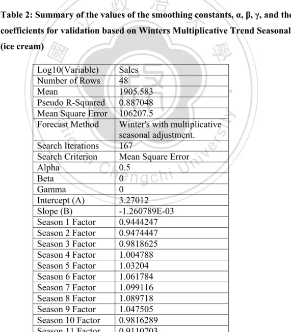
(33) Nov. Dec. 2010 Jan. Feb. Mar Apr. May June July Aug. Sep. Oct. Nov. Dec.. 820 735. 23,225 23,388. 30,200 44,441. 742 936 1,864 1,959 2,096 2,324 3,600 3,226 2,603 1,871 964 780. 21,513 19,069 23,576 24,613 26,646 26,905 27,054 26,610 26,092 26,432 24,471 25,337. 46,198 64,560 96,523 95,333 97,656 87,720 112,769 52,779 35,877 32,687 38,619 69,289. 政治大. 立. 學. ‧ 國. 11 月 12 月 99 年 1月 2月 3月 4月 5月 6月 7月 8月 9月 10 月 11 月 12 月 Source:. 1. Department of Statistics, Ministry of Economic Affairs.www.coa.gov.tw/view.php?catid=7820. ‧. 2. The Industrial Raw Material Price and Volume Information Database (產業原物料價量情報. n. al. er. io. sit. y. Nat. 資料庫, 2011). i n U. 4.2 Results of Forecasting for the Monthly Sales of Ice Cream 4.2.1 Validation. Ch. engchi. v. The monthly market demand from January 2006 to December 2009 (48 months) is used to find the parameters of the forecasting models and validate the projections for the period from January 2010 to December 2010(12 months). In this research, the above sales data was ran using Number Cruncher Statistical System (NCSS) based on two models—winters multiplicative trend seasonal model and the decomposition model. A. Forecast (Validation) Based on Winters Multiplicative Trend Seasonal Model The result was obtained at 11:31:29 PM on 2011/5/15 using NCSS software and summarized as in Table 2. A search is conducted to find the values of the smoothing 25.

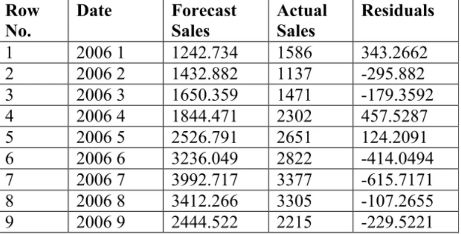
(34) constants that minimize MSE. The Mean Squared Error is 106207.5 and Pseudo RSquared is 0.887048. A value near zero indicates a poorly fitting model, while a value near one indicates a well fitting one. Thus, this model is well fitted. 167 iterations were needed to find the best values for the smoothing constants. The values of the smoothing constants, α, β, and γ are 0.5, 0, and 0, respectively. In the current month, Intercept(A) is 3.27012 and Slope(B) is -1.260789E-03. The seasonal ratios for the next 12 months are also listed from Seasonal 1 Factor to Seasonal 12 Factor. Figure 2 shows the monthly market sales forecast for ice cream in Taiwan.. 治政 Table 2: Summary of the values of the smoothing 大constants, α, β, γ, and the 14 立 based on Winters Multiplicative Trend Seasonal Model coefficients for validation. n. al. Ch. y. sit. io. Search Iterations Search Criterion Alpha Beta Gamma Intercept (A) Slope (B) Season 1 Factor Season 2 Factor Season 3 Factor Season 4 Factor Season 5 Factor Season 6 Factor Season 7 Factor Season 8 Factor Season 9 Factor Season 10 Factor Season 11 Factor. Sales 48 1905.583 0.887048 106207.5 Winter's with multiplicative seasonal adjustment. 167 Mean Square Error 0.5 0 0 3.27012 -1.260789E-03 0.9444247 0.9474447 0.9818625 1.004788 1.03204 1.061784 1.099116 1.089718 1.047505 0.9816289 0.9110703. er. Nat. Log10(Variable) Number of Rows Mean Pseudo R-Squared Mean Square Error Forecast Method. ‧. ‧ 國. 學. (ice cream). engchi. 26. i n U. v.

(35) Season 12 Factor. 0.8986188 Sales Forecast Plot. 4500.0. Sales. 3500.0. 2500.0. 1500.0. 政治大. 500.0 2005.9. 2007.1. 2008.4. 2009.6. Time. 立—Forecast; … Actual Sales. ‧ 國. 學. Figure 2: The monthly market sales and forecasts for ice cream in Taiwan(ton) for validation based on WintersMultiplicativeTrend Seasonal Model.. ‧ sit. y. Nat. Table 3 shows the values of the forecasts, the dates, the actual values, and the. io. (actual – forecast).. n. al. er. residuals. The residual is the difference between the actual sales and the forecast sales. Ch. engchi. i n U. v. Table 3: The monthly market sales for ice cream in Taiwan (forecasts vs. actual) for validation based on WintersMultiplicativeTrend Seasonal Model Row No. 1 2 3 4 5 6 7 8 9. Date 2006 1 2006 2 2006 3 2006 4 2006 5 2006 6 2006 7 2006 8 2006 9. Forecast Sales 1242.734 1432.882 1650.359 1844.471 2526.791 3236.049 3992.717 3412.266 2444.522 27. Actual Sales 1586 1137 1471 2302 2651 2822 3377 3305 2215. Residuals 343.2662 -295.882 -179.3592 457.5287 124.2091 -414.0494 -615.7171 -107.2655 -229.5221. 2010.9.

(36) 政治大. engchi. 28. y. sit. io. Ch. 382.0023 29.46283 12.71842 -52.92105 116.5634 -26.76422 -239.274 199.7294 258.2688 -275.9573 -168.52 -297.7107 62.82398 65.00647 70.76675 -262.4913 -5.69981 58.58673 -183.6525 -258.6176 -8.763535 -297.8171 -149.8065 -136.6507 59.64984 24.67889 -7.778899 23.78662 127.8639 105.6396 37.26005 21.60371 130.4219 1296.522 520.7438 938.982 -529.4974 -120.0931 -63.23501. er. Nat. al. 1807 971 881 1179 1346 1637 1717 2440 3173 3743 3434 2258 1531 949 903 958 1097 1473 1522 1704 2255 2657 2460 1728 1177 714 632 905 1038 1350 1565 1903 2475 4454 4005 3647 1359 820 735. ‧. ‧ 國. 立. 1424.998 941.5372 868.2816 1231.921 1229.437 1663.764 1956.274 2240.271 2914.731 4018.957 3602.52 2555.711 1468.176 883.9935 832.2333 1220.491 1102.7 1414.413 1705.652 1962.618 2263.763 2954.817 2609.806 1864.651 1117.35 689.3211 639.7789 881.2134 910.1361 1244.36 1527.74 1881.396 2344.578 3157.478 3484.256 2708.018 1888.497 940.0931 798.235 1071.611 1092.778 1404.994 1659.212 2022.697 2511.14. 學. 2006 10 2006 11 2006 12 2007 1 2007 2 2007 3 2007 4 2007 5 2007 6 2007 7 2007 8 2007 9 2007 10 2007 11 2007 12 2008 1 2008 2 2008 3 2008 4 2008 5 2008 6 2008 7 2008 8 2008 9 2008 10 2008 11 2008 12 2009 1 2009 2 2009 3 2009 4 2009 5 2009 6 2009 7 2009 8 2009 9 2009 10 2009 11 2009 12 2010 1 2010 2 2010 3 2010 4 2010 5 2010 6. n. 10 11 12 13 14 15 16 17 18 19 20 21 22 23 24 25 26 27 28 29 30 31 32 33 34 35 36 37 38 39 40 41 42 43 44 45 46 47 48 49 50 51 52 53 54. i n U. v.

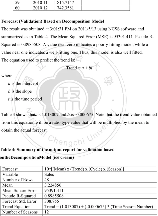
(37) 55 56 57 58 59 60. 2010 7 2010 8 2010 9 2010 10 2010 11 2010 12. 3296.294 3065.983 2239.691 1374.872 815.7147 742.3581. B. Forecast (Validation) Based on Decomposition Model The result was obtained at 3:01:31 PM on 2011/5/13 using NCSS software and summarized as in Table 4. The Mean Squared Error (MSE) is 95391.411. Pseudo RSquared is 0.8985508. A value near zero indicates a poorly fitting model, while a value near one indicates a well-fitting one. Thus, this model is also well fitted.. 政治大 Trend = a + bt. The equation used to predict the trend is:. ‧ 國. 學. where. 立. a is the intercept b is the slope. ‧. t is the time period. y. Nat. sit. Table 4 shows thatais 1.013007 and b is -0.000675. Note that the trend value obtained. al. er. io. from this equation will be a ratio type value that will be multiplied by the mean to. n. obtain the actual forecast.. Ch. engchi. i n U. v. Table 4: Summary of the output report for validation based ontheDecompositionModel (ice cream) Forecast Variable Number of Rows Mean Mean Square Error Pseudo R-Squared Forecast Std. Error Trend Equation Number of Seasons First Year. 10^[(Mean) x (Trend) x (Cycle) x (Season)] Sales 48 3.224856 95391.411 0.8985508 308.855 Trend = (1.013007) + (-0.000675) * (Time Season Number) 12 2006 29.

(38) First Season. 1. Table 5 shows the seasonal component ratios in the Decomposition model. The ratios used to adjust for each season (month or quarter). For example, the last ratio in this example is 0.900578. This indicates that the December correction factor is a 9.9422% decrease in the forecast.. Table 5: Seasonal component ratios for validation based on the Decomposition Model (ice cream) Ratio 0.946733 1.031877 1.048965. No. 2 6 10. 立. No. Ratio 3 0.981609 政治大 7 1.099833. Ratio 0.948577 1.061734 0.983347. 11. No. 4 8 12. 0.913054. Ratio 1.004087 1.091168 0.900578. 學. ‧ 國. No. 1 5 9. Figure 3 shows the monthly market sales forecast for ice cream in Taiwan for validation based on the Decomposition Model. The data plot allows us to analyze. ‧. how closely the forecasts track the data. The plot also shows the forecasts at the end. n. al. Sales. 3500.0. sit. Sales Chart. er. io. 4500.0. y. Nat. of the data series.. Ch. engchi. i n U. v. 2500.0. 1500.0. 500.0 2005.9. 2007.4. 2008.8. Time —Forecast; … Actual Sales 30. 2010.3. 2011.8.

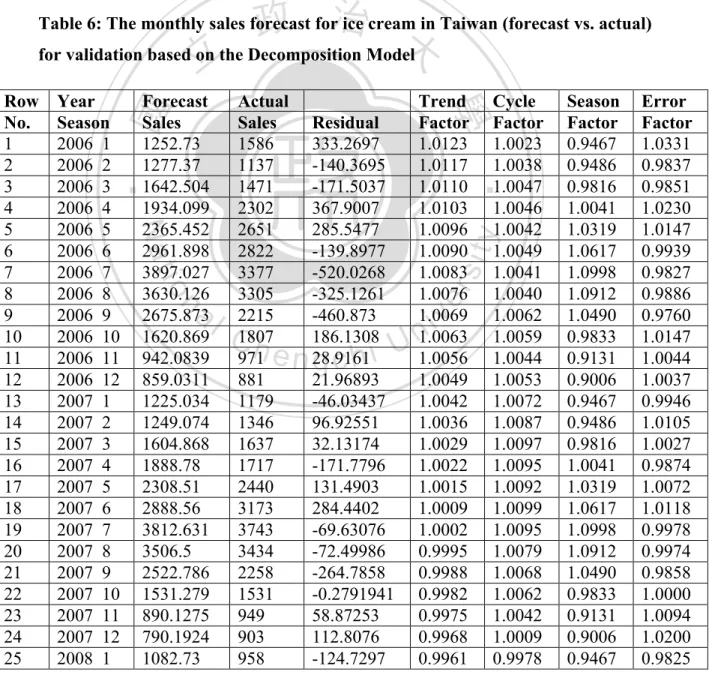
(39) Figure 3: The monthly market sales and forecasts for ice cream in Taiwan(ton) for validation based on the Decomposition Model. Table 6 shows the values of the forecasts, the dates, the actual values, and the residuals for validation based on the Decomposition Model. The residual is the difference between the actual sales and the forecast sales. A value of one is used for all future cycle components. This ignores the cycle in the forecasts, and the random factor is assumed to be one.. 政治大 for validation based on the Decomposition Model 立. Table 6: The monthly sales forecast for ice cream in Taiwan (forecast vs. actual). n. Ch. engchi. 31. Trend Factor 1.0123 1.0117 1.0110 1.0103 1.0096 1.0090 1.0083 1.0076 1.0069 1.0063 1.0056 1.0049 1.0042 1.0036 1.0029 1.0022 1.0015 1.0009 1.0002 0.9995 0.9988 0.9982 0.9975 0.9968 0.9961. Cycle Factor 1.0023 1.0038 1.0047 1.0046 1.0042 1.0049 1.0041 1.0040 1.0062 1.0059 1.0044 1.0053 1.0072 1.0087 1.0097 1.0095 1.0092 1.0099 1.0095 1.0079 1.0068 1.0062 1.0042 1.0009 0.9978. y. sit. Residual 333.2697 -140.3695 -171.5037 367.9007 285.5477 -139.8977 -520.0268 -325.1261 -460.873 186.1308 28.9161 21.96893 -46.03437 96.92551 32.13174 -171.7796 131.4903 284.4402 -69.63076 -72.49986 -264.7858 -0.2791941 58.87253 112.8076 -124.7297. er. ‧ 國. io. al. Actual Sales 1586 1137 1471 2302 2651 2822 3377 3305 2215 1807 971 881 1179 1346 1637 1717 2440 3173 3743 3434 2258 1531 949 903 958. ‧. Forecast Sales 1252.73 1277.37 1642.504 1934.099 2365.452 2961.898 3897.027 3630.126 2675.873 1620.869 942.0839 859.0311 1225.034 1249.074 1604.868 1888.78 2308.51 2888.56 3812.631 3506.5 2522.786 1531.279 890.1275 790.1924 1082.73. 學. Year Season 2006 1 2006 2 2006 3 2006 4 2006 5 2006 6 2006 7 2006 8 2006 9 2006 10 2006 11 2006 12 2007 1 2007 2 2007 3 2007 4 2007 5 2007 6 2007 7 2007 8 2007 9 2007 10 2007 11 2007 12 2008 1. Nat. Row No. 1 2 3 4 5 6 7 8 9 10 11 12 13 14 15 16 17 18 19 20 21 22 23 24 25. i n U. v. Season Factor 0.9467 0.9486 0.9816 1.0041 1.0319 1.0617 1.0998 1.0912 1.0490 0.9833 0.9131 0.9006 0.9467 0.9486 0.9816 1.0041 1.0319 1.0617 1.0998 1.0912 1.0490 0.9833 0.9131 0.9006 0.9467. Error Factor 1.0331 0.9837 0.9851 1.0230 1.0147 0.9939 0.9827 0.9886 0.9760 1.0147 1.0044 1.0037 0.9946 1.0105 1.0027 0.9874 1.0072 1.0118 0.9978 0.9974 0.9858 1.0000 1.0094 1.0200 0.9825.

(40) 2008 2 1068.622 1097 28.37787 0.9955 0.9946 0.9486 1.0038 2008 3 1329.282 1473 143.7183 0.9948 0.9919 0.9816 1.0143 2008 4 1532.883 1522 -10.88312 0.9941 0.9896 1.0041 0.9990 2008 5 1834.214 1704 -130.2142 0.9934 0.9872 1.0319 0.9902 2008 6 2215.919 2255 39.08103 0.9928 0.9842 1.0617 1.0023 2008 7 2866.632 2657 -209.6315 0.9921 0.9826 1.0998 0.9905 2008 8 2678.669 2460 -218.6687 0.9914 0.9826 1.0912 0.9892 2008 9 1961.694 1728 -233.6937 0.9907 0.9825 1.0490 0.9833 2008 10 1217.887 1177 -40.88695 0.9901 0.9828 0.9833 0.9952 2008 11 736.754 714 -22.75405 0.9894 0.9842 0.9131 0.9952 2008 12 678.358 632 -46.35798 0.9887 0.9861 0.9006 0.9891 2009 1 970.5469 905 -65.54693 0.9880 0.9902 0.9467 0.9898 2009 2 1023.457 1038 14.54307 0.9874 0.9966 0.9486 1.0020 2009 3 1370.286 1350 -20.28604 0.9867 1.0043 0.9816 0.9979 2009 4 1678.138 1565 -113.1383 0.9860 1.0100 1.0041 0.9906 2009 5 2086.167 1903 -183.1672 0.9853 1.0123 1.0319 0.9880 2009 6 2636.045 2475 -161.0448 0.9847 1.0147 1.0617 0.9920 2009 7 3512.23 4454 941.7696 0.9840 1.0159 1.0998 1.0291 2009 8 3276.689 4005 728.3111 0.9833 1.0160 1.0912 1.0248 2009 9 2381.017 3647 1265.983 0.9826 1.0159 1.0490 1.0548 2009 10 1460.412 1359 -101.4123 0.9820 1.0162 0.9833 0.9901 2009 11 872.0739 820 -52.07383 0.9813 1.0177 0.9131 0.9909 2009 12 801.1042 735 -66.10418 0.9806 1.0196 0.9006 0.9871 2010 1 981.4221 0.9799 1.0000 0.9467 1.0000 2010 2 989.9675 0.9793 1.0000 0.9486 1.0000 2010 3 1252.561 0.9786 1.0000 0.9816 1.0000 2010 4 1467.416 0.9779 1.0000 1.0041 1.0000 2010 5 1786.271 0.9772 1.0000 1.0319 1.0000 2010 6 2206.635 0.9766 1.0000 1.0617 1.0000 2010 7 2892.841 0.9759 1.0000 1.0998 1.0000 2010 8 2701.978 0.9752 1.0000 1.0912 1.0000 2010 9 1980.025 0.9746 1.0000 1.0490 1.0000 2010 10 1225.491 0.9739 1.0000 0.9833 1.0000 2010 11 733.7712 0.9732 1.0000 0.9131 1.0000 2010 12 667.4899 0.9725 1.0000 0.9006 1.0000 Note: This section shows the values of the forecasts, the dates, the actual values, the. 立. 政治大. ‧. ‧ 國. 學. n. al. er. io. sit. y. Nat. 26 27 28 29 30 31 32 33 34 35 36 37 38 39 40 41 42 43 44 45 46 47 48 49 50 51 52 53 54 55 56 57 58 59 60. Ch. engchi. i n U. v. residuals, and the forecast ratios. A value of one is used for all future cycle components. This ignores the cycle in the forecasts. And the random factor is assumed to be one. From Table 7 and Table 8, we compare the MSEs for forecasts based on two models—the Winters Multiplicative Trend Seasonal Model and the Decomposition 32.

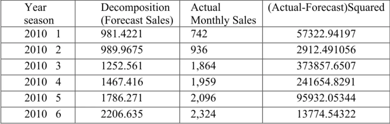
(41) Model. It shows that the Decomposition Model generates better forecasts than those from Winters Multiplicative Trend Seasonal Model. Therefore, we complete the validation procedure.. Table 7: MSE of forecast for validation based on Winters Multiplicative Trend Seasonal Model (ice cream). 742 936 1,864 1,959 2,096 2,324 3,600 3,226 2,603 1,871 964 780. 政治大. 108643.4113 24579.34128 210686.508 89872.84494 5373.329809 35021.3796 92237.33444 25605.44029 131993.4295 246142.9924 21988.5302 1416.912636 MSE (winter's trend) 82,796.79. 學. y. ‧. er. n. al. (Actual-Forecast)Squared. sit. 立. io. 1 2 3 4 5 6 7 8 9 10 11 12. Actual Monthly Sales. Nat. 2010 2010 2010 2010 2010 2010 2010 2010 2010 2010 2010 2010. Winter's Trend Seasonal (Forecast Sales) 1071.611 1092.778 1404.994 1659.212 2022.697 2511.14 3296.294 3065.983 2239.691 1374.872 815.7147 742.3581. ‧ 國. Year season. Ch. engchi. i n U. v. Table 8: MSE of Forecast for validation based on the Decomposition Model (ice cream) Year season 2010 1 2010 2 2010 3 2010 4 2010 5 2010 6. Decomposition (Forecast Sales) 981.4221 989.9675 1252.561 1467.416 1786.271 2206.635. Actual Monthly Sales 742 936 1,864 1,959 2,096 2,324 33. (Actual-Forecast)Squared 57322.94197 2912.491056 373857.6507 241654.8291 95932.05344 13774.54322.

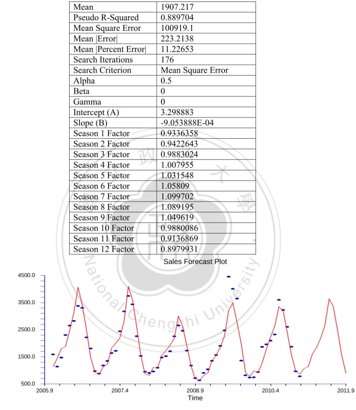
(42) 2010 2010 2010 2010 2010 2010. 7 8 9 10 11 12. 2892.841 2701.978 1980.025 1225.491 733.7712 667.4899. 3,600 3,226 2,603 1,871 964 780. 500073.8513 274599.0565 388097.8506 416681.8691 53005.30035 12658.5226 MSE (decomposition) 202,547.58. 4.2.2 Forecasts. 治政 2009 (48 months) of ice cream,the Winters multiplicative trend 大seasonal model is selected as the forecasting model to project the立 sales of next 12 months. In this section, we will use theWinters After the validation procedures on the monthly market sales from January 2006 to December. ‧ 國. 學. model to generate forecasts for the period from January 2011 to December 2011(12 months). The result was obtained at11:39:18 PM on 2011/5/15 using NCSS software and summarized as. ‧. in Table 9. A search is conducted to find the values of the smoothing constants that minimize MSE. The mean square error is 100919.1 and Pseudo R-Squared is 0.889704. A value near zero. y. Nat. sit. indicates a poorly fitting model, while a value near one indicates a well-fitting one. Thus, this. al. er. io. model is well-fitted. 176 iterations were required to find the best values for the smoothing. n. constants. The values of the smoothing constants, α, β, γ, are 0.5, 0, 0, respectively. In the current. Ch. i n U. month, Intercept(A) is 3.298883 and Slope(B) is -9.053888E-04.. engchi. v. Figure 4 shows the monthly market sales forecasts for ice cream in Taiwan. Table 9: Summary of the values of the smoothing constants, α, β, γ, and the 14 coefficients for forecasting based on Winters Multiplicative Trend Seasonal Model (ice cream) Forecast Method. Winter's with multiplicative seasonal adjustment. Forecasts are made for the period from January 2011 to December 2011(12 months) Forecast Summary Section Log10(Variable) Sales Number of Rows 60 34.

(43) Mean Pseudo R-Squared Mean Square Error Mean |Error| Mean |Percent Error| Search Iterations Search Criterion Alpha Beta Gamma Intercept (A) Slope (B) Season 1 Factor Season 2 Factor Season 3 Factor Season 4 Factor Season 5 Factor Season 6 Factor Season 7 Factor Season 8 Factor Season 9 Factor Season 10 Factor Season 11 Factor Season 12 Factor. 政治大. sit. y. Sales Forecast Plot. n. al. er. io. Sales. ‧. Nat. 3500.0. 學. ‧ 國. 立. 4500.0. 1907.217 0.889704 100919.1 223.2138 11.22653 176 Mean Square Error 0.5 0 0 3.298883 -9.053888E-04 0.9336358 0.9422643 0.9883024 1.007955 1.031548 1.05809 1.099702 1.089195 1.049619 0.9880086 0.9136869 0.8979931. Ch. 2500.0. engchi. i n U. v. 1500.0. 500.0 2005.9. 2007.4. 2008.9. 2010.4. Time. —Forecasts; … Actual Sales Figure 4: The monthly market sales forecast for ice cream in Taiwan(ton) based on Winters Multiplicative Trend Seasonal Model. 35. 2011.9.

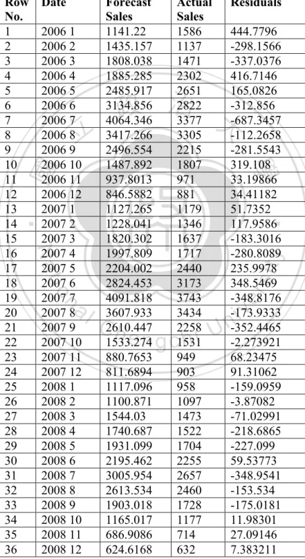
(44) Table 10 shows the values of the forecasts, the dates, the actual values, and the residuals. The residual is the difference between the actual sales and the forecast sales (actual-forecast). Table 10: The monthly market sales for ice cream in Taiwan (forecast vs actual) based on Winters Multiplicative Trend Seasonal Model. io. n. 444.7796 -298.1566 -337.0376 416.7146 165.0826 -312.856 -687.3457 -112.2658 -281.5543 319.108 33.19866 34.41182 51.7352 117.9586 -183.3016 -280.8089 235.9978 348.5469 -348.8176 -173.9333 -352.4465 -2.273921 68.23475 91.31062 -159.0959 -3.87082 -71.02991 -218.6865 -227.099 59.53773 -348.9541 -153.534 -175.0181 11.98301 27.09146 7.383211. 政治大. Ch. engchi. 36. y. Nat. al. Residuals. sit. ‧ 國. 立. Actual Sales 1586 1137 1471 2302 2651 2822 3377 3305 2215 1807 971 881 1179 1346 1637 1717 2440 3173 3743 3434 2258 1531 949 903 958 1097 1473 1522 1704 2255 2657 2460 1728 1177 714 632. ‧. 2006 1 2006 2 2006 3 2006 4 2006 5 2006 6 2006 7 2006 8 2006 9 2006 10 2006 11 2006 12 2007 1 2007 2 2007 3 2007 4 2007 5 2007 6 2007 7 2007 8 2007 9 2007 10 2007 11 2007 12 2008 1 2008 2 2008 3 2008 4 2008 5 2008 6 2008 7 2008 8 2008 9 2008 10 2008 11 2008 12. Forecast Sales 1141.22 1435.157 1808.038 1885.285 2485.917 3134.856 4064.346 3417.266 2496.554 1487.892 937.8013 846.5882 1127.265 1228.041 1820.302 1997.809 2204.002 2824.453 4091.818 3607.933 2610.447 1533.274 880.7653 811.6894 1117.096 1100.871 1544.03 1740.687 1931.099 2195.462 3005.954 2613.534 1903.018 1165.017 686.9086 624.6168. er. Date. 學. Row No. 1 2 3 4 5 6 7 8 9 10 11 12 13 14 15 16 17 18 19 20 21 22 23 24 25 26 27 28 29 30 31 32 33 34 35 36. i n U. v.

(45) 95.18927 128.5797 -6.91211 6.166496 51.7087 201.3322 1241.145 516.3934 880.9222 -615.4746 -116.9445 -43.76217 -240.3508 29.07175 580.5806 172.8543 -130.5196 -302.3345 248.5954 20.09929 210.1373 297.4036 -14.01678 -81.17062. 政治大. n. Ch. engchi. y. sit er. io. al. 905 1038 1350 1565 1903 2475 4454 4005 3647 1359 820 735 742 936 1864 1959 2096 2324 3600 3226 2603 1871 964 780. ‧. ‧ 國. 立. 809.8107 909.4203 1356.912 1558.833 1851.291 2273.668 3212.855 3488.607 2766.078 1974.475 936.9445 778.7621 982.3508 906.9282 1283.419 1786.146 2226.52 2626.334 3351.405 3205.901 2392.863 1573.596 978.0168 861.1707 1067.558 1136.387 1599.269 1848.076 2199.113 2674.779 3639.806 3357.914 2494.585 1572.923 902.4263 801.3745. 學. 2009 1 2009 2 2009 3 2009 4 2009 5 2009 6 2009 7 2009 8 2009 9 2009 10 2009 11 2009 12 2010 1 2010 2 2010 3 2010 4 2010 5 2010 6 2010 7 2010 8 2010 9 2010 10 2010 11 2010 12 2011 1 2011 2 2011 3 2011 4 2011 5 2011 6 2011 7 2011 8 2011 9 2011 10 2011 11 2011 12. Nat. 37 38 39 40 41 42 43 44 45 46 47 48 49 50 51 52 53 54 55 56 57 58 59 60 61 62 63 64 65 66 67 68 69 70 71 72. i n U. v. 4.3 Results of Forecasting for the Monthly Sales of Fresh Milk 4.3.1 Validation The monthly market demand from January 2006 to December 2009 (48 months) of fresh milk is used to find the parameters of the forecasting models and validate the projections for the period 37.

(46) from January 2010 to December 2010(12 months). In this research, the above sales data was ran using Number Cruncher Statistical System (NCSS) based on the same two models that was also used for ice cream—winters multiplicative trend seasonal model and the decomposition model. A. Forecast (Validation) Based on Winters Multiplicative Trend Seasonal Model The result was obtained at4:52:29 PM on 2011/6/11 using NCSS software and summarized as in Table 11. A search is conducted to find the values of the smoothing constants that minimize MSE. The Mean Squared Error is 790666.8 and Pseudo RSquared is 0.914516. A value near zero indicates a poorly fitting model, while a value near one indicates a well fitting one. Thus, this model is well fitted. 151 iterations. 政治大. were needed to find the best values for the smoothing constants. The values of the smoothing constants, α, β, and γ are 0.8145158, 5.716994E-08, and 2.286691E-03,. 立. respectively. In the current month, Intercept(A) is 4.380449 and Slope(B) is. ‧ 國. 學. 1.021276E-04.. The seasonal ratios for the next 12 months are also listed from Seasonal 1 Factor to. ‧. Seasonal 12 Factor.. Figure 5 shows the monthly market sales forecast for fresh milk in Taiwan.. sit. y. Nat. al. er. io. Table 11: Summary of the values of the smoothing constants, α, β, γ, and the 14. n. coefficients for validation based on Winters Multiplicative Trend Seasonal Model (fresh milk). Ch. Forecast Method Log10(Variable) Number of Rows Mean Pseudo R-Squared Mean Square Error Mean |Error| Mean |Percent Error| Search Iterations Search Criterion Alpha Beta. engchi. i n U. v. Winter's with multiplicative seasonal adjustment. Sales 48 22284.81 0.914516 790666.8 723.2148 3.293337 151 Mean Square Error 0.8145158 5.716994E-08 38.

(47) Gamma Intercept (A) Slope (B) Season 1 Factor Season 2 Factor Season 3 Factor Season 4 Factor Season 5 Factor Season 6 Factor Season 7 Factor Season 8 Factor Season 9 Factor Season 10 Factor Season 11 Factor Season 12 Factor. 立. ‧ 國. ‧. io. y. sit. 18000.0. n. al. er. 22000.0. Sales Forecast Plot. Nat. Sales. 26000.0. 政治大. 學. 30000.0. 2.286691E-03 4.380449 1.021276E-04 0.9797085 0.9726461 0.9911656 0.9972439 1.007274 1.00772 1.015774 1.015128 1.01006 1.009061 0.9990233 0.9951959. 14000.0 2005.9. Ch. 2007.1. engchi. i n Time U. 2008.4. v. 2009.6. —Forecasts; … Actual Sales Figure 5: The monthly sales and forecasts for fresh milk in Taiwan(ton) for validation based on Winters Multiplicative Trend Seasonal Model.. Table 12 shows the values of the forecasts, the dates, the actual values, and the residuals. The residual is the difference between the actual sales and the forecast sales (actual – forecast).. 39. 2010.9.