Monte Carlo simulation of the motions associated with a single Rouse segment
Y.-H. Lin and Z.-H. LuoCitation: The Journal of Chemical Physics 112, 7219 (2000); doi: 10.1063/1.481286 View online: http://dx.doi.org/10.1063/1.481286
View Table of Contents: http://scitation.aip.org/content/aip/journal/jcp/112/16?ver=pdfcov
Published by the AIP Publishing
Articles you may be interested in
Monte Carlo simulation of homopolymer chains. I. Second virial coefficient
J. Chem. Phys. 118, 4721 (2003); 10.1063/1.1543940
Effect of twisting on the behavior of a double-stranded polymer chain: A Monte Carlo simulation
J. Chem. Phys. 111, 9424 (1999); 10.1063/1.480035
Monte Carlo simulation of self-avoiding lattice chains subject to simple shear flow. I. Model and simulation algorithm
J. Chem. Phys. 107, 4070 (1997); 10.1063/1.474763
On lyotropic behavior of molecular bottle-brushes: A Monte Carlo computer simulation study
J. Chem. Phys. 107, 3267 (1997); 10.1063/1.474677
Monte Carlo simulation of polymer chain collapse in an athermal solvent
J. Chem. Phys. 106, 1288 (1997); 10.1063/1.473225
Monte Carlo simulation of the motions associated
with a single Rouse segment
Y.-H. Lina) and Z.-H. Luo
Department of Applied Chemistry, National Chiao Tung University, Hsinchu, Taiwan, Republic of China
共Received 27 July 1999; accepted 1 February 2000兲
The validity of the Monte Carlo simulation for studying the dynamics of a Rouse chain with a finite number of beads, N, is established by showing the close agreement between the simulation results and the analytical solutions for the time-correlation function of the end-to-end vector. Then, the Monte Carlo simulation is used to calculate the dynamic functions associated with the bond vector b(t) or direction u(t)⫽b(t)/兩b(t)兩 of an elastic dumbbell and a Rouse segment in a chain. The effect of chain connectivity on the motions of a single Rouse segment is studied. In particular, it is shown that the dynamic function
具
P2关u(0)•u(t)兴典
2 over a wide dynamic range, which is the main region probed by the depolarized photon-correlation spectroscopy, is basically independent of the values of N⭓8 in agreement with the experimental results. Furthermore, the line shape of the depolarized photon-correlation functions of the concentrated solutions共⬇60 wt. %兲 of polystyrene in cyclohexane at the theta point can be fully accounted for by including the effect of chain connectivity regardless of the crudeness of the Rouse segment relative to the chemical structure. From this study, the molecular weight for a Rouse segment of polystyrene in the concentrated solutions is estimated to be 1100, which is slightly larger than the values m⫽780– 900 obtained for polystyrene in the melt state by other methods. © 2000 American Institute of Physics.关S0021-9606共00兲50316-X兴 INTRODUCTION
Slow polymer dynamic and viscoelastic behavior in an entanglement-free system can be well described by theories developed in terms of the Rouse segment as the basic struc-tural unit.1–3If our interest is not limited to the slow modes of motions of a long polymer chain, we have to ask how short the Rouse segment can be as it is defined statistically. Related to this is the early studies of the Kuhn segment 共con-sidered as equivalent to the Rouse segment兲 based on the determination of the persistence length by neutron scattering.4,5 In the recent years, there was much research interest in the subject; and different approaches had been taken:共1兲 The Rouse segment size was calculated from the high frequency rubbery modulus determined by analyzing the measured dynamic viscoelastic and birefringence spectra with the assumption of a modified stress-optical rule for glassy polymer.6,7共2兲 Through a theoretical analysis relating the depolarized photon-correlation and viscoelastic results of a polystyrene melt, the dynamics and size of a ‘‘Rouse’’ segment can be studied.8–10 共3兲 The line shapes of the vis-coelastic spectra of a series of the polystyrene blends in the entanglement-free region have been analyzed in terms of the Rouse model for the high-molecular-weight component and the elastic dumbbell model for the low-molecular-weight component. The best value for the Rouse segment size oc-curs, when the viscoelastic spectrum is best described by the theory in both the low and high frequency regions corre-sponding to the viscoelastic responses of the high- and small-molecular weight components, respectively.11The values for
the molecular weight of a Rouse segment of polystyrene ob-tained by these studies range from 780 to 900.
In the second approach listed above, it has been shown that the collective motion observed by the depolarized Ray-leigh is basically that associated with a Rouse segment. If each Rouse segment is treated as an elastic dumbbell and undergoes the freely rotational diffusion motion, the correla-tion time r for
具
P2关u(0)•u(t)兴典
关where u(t) is the unitvector indicating the orientation of the Rouse segment; and
P2 is the second-order Legendre polynomial兴, which is the
dynamic function probed by the depolarized photon-correlation spectroscopy, can be obtained to be
r⫽
⬘具
b2典
/18kT⫽具
b2典
/36kT, 共1兲 where⬘
is the friction constant experienced by each bead on the elastic dumbbell, which is half the friction constantfor each bead on the Rouse chain (/⬘
⫽2, because the mass of an elastic dumbbell is treated as equivalent to that of a Rouse segment; and the mass of the bead of the former is half that of the latter兲. On the other hand, the relaxation time of the highest Rouse viscoelastic mode is given byv⫽
具
b2典
/24kT⫽K2m2/24 共2兲with the friction factor K given by
K⫽
具
b2典
/kT2m2, 共3兲where m is the molecular weight of a Rouse segment.12,13 With the m value known,v can be calculated from the vis-coelastic data, such as the zero shear viscosity, which is given by
0⫽共cRT2/36兲KM, 共4兲
where c is the weight amount of polymer per unit volume; and M the molecular weight of the polymer sample.
a兲Author to whom correspondence should be addressed.
7219
0021-9606/2000/112(16)/7219/8/$17.00 © 2000 American Institute of Physics
Equations共1兲 and 共2兲 indicates that the two characteristic time constants as can be obtained by the depolarized photon-correlation and viscoelasticity measurements have the same temperature dependence 共that of, which is often described by the WLF equation14兲 and the same order of magnitude. These expectations have been supported by the results of the depolarized photon-correlation and viscoelasticity measure-ments.
In obtaining Eq.共1兲, the connections of each Rouse seg-ment in both ends to the rest of the chain are neglected. The connection of the Rouse segments in a chain gives rise to the Rouse normal modes of motions. Based on the Rouse model, the viscoelastic spectrum and the time correlation function of the end-to-end vector can be theoretically expressed in terms of the normal modes.1–3 The dynamic functions,
具
us(0) •us(t)典
and具
P2关us(0)•us(t)兴典
associated with a single Rouse segment, which do not have an analytical solution, can be calculated by the Monte Carlo simulation based on the Langevin equation.With the effect of the connection between neighboring Rouse segments included, any dynamic function associated with a single Rouse segment is expected to be nonsingle-exponential. It is well known that the depolarized photon-correlation function of a polymer melt or concentrated solu-tion is not a single exponential.15,16This study allows us to study the chain connectivity in affecting the non-single-exponential decaying behavior.
First, we shall establish the validity of the Monte Carlo simulation by the comparison with the analytical solution for the time-correlation function of the end-to-end vector
具
R(0)•R(t)典
of a Rouse chain with a finite number of beads,N. Then we can use the Monte Carlo simulation to calculate
the time correlation functions,
C0s共t兲⫽
具
bs共0兲•bs共t兲典
/具
bs 2典
, 共5兲 C1s共t兲⫽具
us共0兲•us共t兲典
共6兲 and C2s共t兲⫽具
P2关us共0兲ўus共t兲典
兴, 共7兲where bs(t) is the bond vector of the sth Rouse segment at time t and us(t)⫽bs(t)/兩bs(t)兩. Before the effect of chain connectivity as reflected by the above dynamic functions is studied, we shall examine by the Monte Carlo simulation how well in the elastic dumbbell case C0(t)⫽
具
b(0) •b(t)典
/具
b2典
can be approximated by C1(t)⫽具
u(0)•u(t)典
关where u(t)⫽b(t)/兩b(t)兩] and how applicable is the freely rotational diffusion model in relating C0(t) 关or C1(t)] and C2(t)⫽具
P2关u(0)•u(t)兴典
. And finally the average⌺s⫽1,N⫺1C2s(t)/(N⫺1) in a Rouse chain will be studied as
a function of N and compared with the results of the depo-larized photon-correlation measurements.
THE LANGEVIN EQUATION
Consider a linear Gaussian chain with N beads, whose configuration is represented by the set of N position vectors of the beads 兵Rn其⬅(R1,R2,R3,...,RN). While the move-ment of each bead is hindered by a friction force character-ized by the friction constant, it receives the random force
fn(t)⫽(gn(t)) due to the incessant collisions of the bead 共the Brownian particle兲 with the fluid molecules or segments. Then the motions of the chain are described by the Langevin equations2,9
dRn/dt⫽⫺共3kT/
具
b2典
兲共2Rn⫺Rn⫹1⫺Rn⫺1兲⫹gn共t兲 共8兲 for the internal beads (n⫽2,3,4,...,N⫺1) and
dR1/dt⫽⫺共3kT/
具
b2典
兲共R1⫺R2兲⫹g1共t兲, 共9兲
dRN/dt⫽⫺共3kT/
具
b2典
兲共RN⫺RN⫺1兲⫹gN共t兲, 共10兲 for the end beads (n⫽1 and N兲. The random fluctuation gnis Gaussian and characterized by the moments具
gn共t兲典
⫽0, 共11兲具
gn␣共t兲gm共t⬘
兲典
⫽2D␦nm␦␣␦共t⫺t⬘
兲, 共12兲 where D(⫽kT/) is the diffusion constant of a free bead; and␣,represent the x, y, z coordinates.The bond vectors 兵bs其 and the end-to-end vector R are defined, respectively, as
bs⫽Rs⫹1⫺Rs, 共13兲
R⫽RN⫺R1⫽⌺s⫽1,N⫺1bs. 共14兲
Following the usual procedure of transformation to the normal coordinates,1,17 the time correlation function of the end-to-end vector R(t) is obtained as
具
R共0兲•R共t兲典
⫽⌺p⫽odd,1 to N⫺1共2具
b2典
/N兲 ⫻关cos2共p/2N兲/sin2共p/2N兲兴⫻exp共⫺t/p兲 共15兲
with⌺p⫽odd,1 to N⫺1meaning summation over odd p’s from 1 to N⫺1, and
p⫽
具
b2典
/关12kT sin2共p/2N兲兴⫽K2M2/关12N2sin2共p/2N兲兴, 共16兲
where K is given by Eq.共3兲.
When N→⬁, Eq. 共15兲 in combination with Eq. 共16兲 re-duces to the result obtained from the continuous Rouse chain model.2
The time correlation function of bs(t) 关Eq. 共5兲兴 is ob-tained in terms of the normal modes as
C0s共t兲⫽共2/N兲⌺p⫽1,N⫺1sin2共sp/N兲exp共⫺t/p兲. 共17兲
THE MONTE CARLO SIMULATION
In the Monte Carlo simulation, the Langevin equation is replaced by the calculation of the positions of the beads at the next step 兵Rn(ti⫹⌬t)其 from their positions 兵Rn(ti)其 at some present time ti共note ti⫹1⫽ti⫹⌬t).18,19Corresponding to Eq.共8兲,
R共ti⫹⌬t兲⫽R共ti兲⫺S关2Rn共ti兲⫺Rn⫹1共ti兲⫺Rn⫺1共ti兲兴⫹dni, 共18兲 where
S⫽3D⌬t/
具
b2典
, 共19兲7220 J. Chem. Phys., Vol. 112, No. 16, 22 April 2000 Y.-H. Lin and Z.-H. Luo
and the random displacement dni is Gaussian and character-ized by the moments,
具
dni典
⫽0, 共20兲具
d␣nidm j典⫽␦␣,␦n,m␦i, j2D⌬t, 共21兲 where ␣,  represent the x,y,z coordinates 共for instance dx represent the x-component of d兲. Equations equivalent to Eq. 共18兲 can similarly be written for Eqs. 共9兲 and 共10兲. Depen-dent on the choice of 2D⌬t⫽l2 in the Monte Carlo simula-tion, the number of time steps corresponding top关Eq. 共16兲兴 is given byp/⌬t⫽共
具
b2典
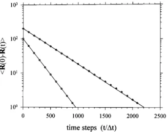
/l2兲/6 sin2共p/2N兲. 共22兲 COMPARISON OF THE SIMULATION RESULTS AND THE ANALYTICAL SOLUTIONSWe have chosen the simple chain systems, N⫽2, 3, and 5 for making the comparison between simulation and theory. According to Eq.共15兲, only a single relaxation mode occurs in the time correlation function of the end-to-end vector in either the N⫽2 or the N⫽3 system; and two relaxation modes in the case of N⫽5. Shown in Fig. 1 are the compari-sons of the simulation results of N⫽2 and N⫽3 with Eq. 共15兲 in combination with Eq. 共22兲. The chosen parameters in the simulation are
具
b2典
0.5⫽10, and l⫽0.4. The shownsimu-lation results are the outcomes of averaging over 4⫻108
steps. As shown in Fig. 1 for N⫽2 and 3, both the initial values and the relaxation times obtained from the simulation are in close agreement with the theoretical results. In the case of N⫽5, similar close agreement between theory and simu-lation is obtained. The results shown in Figs. 1 as well as that obtained for N⫽5 illustrate that the chain dynamics as de-scribed by the Langevin equations 关Eqs. 共8兲–共12兲兴 can be faithfully calculated by the Monte Carlo simulation. Thus, the Monte Carlo simulation can be used to calculate dynamic functions of a physical quantity or of a system with addi-tional effects, which are impossible to obtain analytically.
THE MOTION OF AN ELASTIC DUMBBELL
The elastic dumbbell model is a special case of the Rouse chain model. The dynamic behavior C0(t)⫽
具
b(0)•b(t)
典
/具
b2典
关Eq. 共5兲兴 for the elastic dumbbell can beob-tained from the Langevin equations to be a single exponen-tial decay as shown in Fig. 1. C0(t) being a single
exponen-tial decay suggests that the elastic dumbbell motion may be sufficiently well described by the free rotational diffusion model. Based on the freely rotational diffusion model,20the dynamic function C2(t)⫽
具
P2关u(0)•u(t)兴典
关Eq. 共7兲兴 isex-pected to be a single exponential decay with the relaxation time being one third of that of C0(t)关see Eq. 共1兲兴. How well the free rotational diffusion model describe C2(t) of an elas-tic dumbbell can be studied by the Monte Carlo simulation. However, in the simulation calculation of C2(t), we need to
assume u(t)⫽b(t)/兩b(t)兩. From comparing Eqs. 共5兲 and 共7兲, this means that we have assumed that b(t)/
具
b2典
0.5 can be approximated by u(t)⫽b(t)/兩b(t)兩. We can test this ap-proximation by showing that C0(t) can be wellapproxi-mated by C1(t)⫽
具
u(0)•u(t)典
关Eq. 共6兲兴.The relation between C1(t) and C0(t) can be analyzed
as in the following. Denoting兩b(t)兩 as b(t) and
具
兩b兩典
as b0,we may express b(t) as
b共t兲⫽b0⫹⌬b共t兲, 共23兲
where⌬b(t) is the bond length fluctuation. For
具
b2典
⫽100 asassumed in this study, we have obtained b0⫽9.2, which is
not much smaller than
具
b2典
0.5. This indicates that the fluc-tuation⌬b(t) is rather small. This is the main basis for our approximating C0(t) by C1(t) and treating the Rouseseg-ment basically as equivalent to a Kuhn segseg-ment 共for in-stance, when we relate the viscoelastic data to the depolar-ized photon correlation results兲. Using Eq. 共23兲, C1(t) can be
approximately expressed as C1共t兲⬇
具
b共0兲•b共t兲典具
1/关b共0兲b共t兲兴典
⫽具
b共0兲•b共t兲典具
1/关共b0⫹⌬b共0兲兲共b0⫹⌬b共t兲兲兴典
⫽具
b共0兲•b共t兲典具
1/关b02共1⫹⌬b共0兲/b0兲 ⫻共1⫹⌬b共t兲/b0兲兴典
⬇具
b共0兲•b共t兲典具
共1⫺⌬b共0兲/b0兲 ⫻共1⫺⌬b共t兲/b0兲典
/具
b2典
⫽C0共t兲关1⫹具
⌬b共0兲⌬b共t兲典
/b0 2 兴. 共24兲Equation 共24兲 mainly shows the dynamic relation between
C1(t) and C0(t). Both C1(t) and C0(t) as they are defined
are normalized functions. Because of the approximation steps taken, C1(t) as expressed by Eq. 共24兲 is not
normal-ized; and need be renormalized. As shown in Fig. 2, after a small initial drop due to the decay of
具
⌬b(0)⌬b(t)典
/b02, the relaxation curves of C1(t) and C0(t) parallel each other andmaintain a ratio C1(t)/C0(t)⫽0.85. It is also shown in Fig. 2
that the agreement between C1(t) obtained directly from the
simulation and C1(t) calculated from Eq. 共24兲 using the
simulation results of C0(t) and
具
⌬b(0)⌬b(t)典
andrenor-malized is very good.
FIG. 1. Comparison of the analytical solution共the solid line兲 and the Monte Carlo simulation for the time correlation function of the end-to-end vector
R(t) of the Rouse chain with N⫽2 共䊊兲 and with N⫽3 共〫兲.
Also shown in Fig. 2 is the comparison of the theoretical curve of C2(t) based on using the free rotational diffusion model in relating C0(t) and C2(t), and the simulation curve
of C2(t). One can notice that in the short time region共down
to C2(t)⫽0.3⬇e⫺1), the simulation result of C2(t) can be
well described by the free rotational diffusion model, while, the whole simulated C2(t) curve is not a single exponential
decay. Overall, the elastic dumbbell dynamic behavior is not far from described by the free rotational diffusion model as revealed in terms of the comparison of C0(t)关or C1(t)] and C2(t). The simulation result of C2(t) in particular will serve
as a reference for comparison with the dynamic behavior of a Rouse segment in a chain to study the effect of chain con-nectivity.
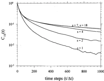
THE MOTION OF A ROUSE SEGMENT IN A CHAIN As expected intuitively, the simulated C0s(t), C1s(t),
and C2s(t) dynamic processes become slower gradually, as
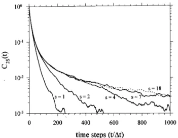
the monitored segment 共denoted by the index s兲 is shifted from the chain end to the middle of the chain as shown in Figs. 3, 4, and 5 共to avoid congestion in the figures, only results at a few selected s values are shown兲. The shown results for a chain with N⫽36 indicate that the dynamic functions over the whole range become basically indepen-dent of s for s⫽7 – 18. In other words, the dynamic functions of a segment, which is only a few segments away from the chain end is free of the chain end effect and become inde-pendent of s. In particular, C2s(t) over a wide of dynamic
range共⬇one and a half orders兲 is very much independent of
s for s⭓2. It is shown in Fig. 3 that the simulation results of C0s(t) at different s values are in close agreement with the
curves calculated from Eq. 共17兲. As expected, the dynamic functions obtained from the simulation are symmetric with respect to the center of the chain i.e., the dynamic function at the sth segment is the same as that at the (N-s)th segment.
Experimentally 共for example, in the depolarized photon-correlation spectroscopy兲, it is often the average of the dy-namic functions, that are probed. Thus, we define
具
C0共t兲典
⫽共⌺s⫽1,N⫺1C0s共t兲兲/共N⫺1兲, 共25兲具
C1共t兲典
⫽共⌺s⫽1,N⫺1C1s共t兲兲/共N⫺1兲, 共26兲and
具
C2共t兲典
⫽共⌺s⫽1,N⫺1C2s共t兲兲/共N⫺1兲. 共27兲Shown in Fig. 6 is the comparison of
具
C0(t)典
,具
C1(t)典
, and具
C2(t)典
for a chain with N⫽36. While具
C0(t)典
is no longera single exponential decay as C0(t), the relative differences
among
具
C0(t)典
,具
C1(t)典
, and具
C2(t)典
are similar to thoseamong C0(t), C1(t), and C2(t) as shown in Fig. 2 for the
elastic dumbbell case.
FIG. 2. Comparison of the analytic solution共the upper solid line兲 and the simulation共䊊兲 for C0(t); comparison of C1(t) obtained directly from
simu-lation共䉭兲 and calculated from Eq. 共24兲 using the simulation results of C0(t)
and 具⌬b(0)⌬b(t)典 共the lower solid line兲; Comparison of C2(t) obtained
from simulation共䊐兲 and expected based on C0(t) and the freely rotational
diffusion model共•• –兲. All the shown dynamic functions are for the elastic dumbbell.
FIG. 3. Comparison of the simulation results of C0s(t)共䊊 for s⫽1; 䉮 for
s⫽2; 䊐 for s⫽4; 䉭 for s⫽7; and 〫 for s⫽18) and those calculated from Eq.共17兲 for the Rouse chain with N⫽36 共the solid lines from left to right are for s⫽1, 2, 4, and 7 respectively; while the dotted line is for s⫽18, which is virtually superposed on the line for s⫽7). The simulation results are symmetrical with respect to the center of the chain; and the results of only one side are shown.
FIG. 4. The simulation results of C1s(t) as a function of s共the solid lines
from left to right are for s⫽1, 2, 4, and 7, respectively, while the dotted line is for s⫽18).
7222 J. Chem. Phys., Vol. 112, No. 16, 22 April 2000 Y.-H. Lin and Z.-H. Luo
What is particularly interesting to us is the
具
C2(t)典
dy-namic process for comparison with the depolarized photon-correlation results. The dynamic function directly observed from the photon-correlation spectroscopy is the square of具
C2(t)典
. In Fig. 7, we show the comparison of the具
C2(t)典
2curves calculated for N⫽2, 8, 16, and 36. It can be seen that the relaxation time distributions for N⫽8, 16, and 36 is sig-nificantly broader than that of the elastic dumbbell case (N ⫽2) and that in the short time region 共down to
具
C2(t)典
2⫽0.01), basically there is no difference among the curves for different values of N⭓8. Mainly the tail region of the relaxation curve is slowly moved to the longer time with increasing N. In other words, the short time region of
具
C2(t)典
2 is mainly affected by the local motion, which isindependent of the molecular weight, the tail region of the relaxation curve is weakly affected by the slow modes of the Rouse chain, which is molecular weight dependent. As
C2s(t) is least dependent on s over a large dynamic range as
pointed out above,
具
C2(t)典
is much less affected by themo-lecular weight change than
具
C0(t)典
and具
C1(t)典
.In the depolarized photon-correlation spectroscopy, it is mainly the short time region of
具
C2(t)典
2 that is probed.9,10
The above result is in agreement with the basic molecular weight independence of the depolarized photon-correlation function, that has been observed.
COMPARISON OF SIMULATION AND EXPERIMENT FORŠC2„t…‹2
In a polymer system, the static pair correlation as deter-mined from the depolarized intensity measurement is often expressed in terms of effective optical anisotropy ␦2 per
monomer unit to account for the concentration dependence of the measured total intensity. In the case of polystyrene,21,22it has been shown that the ␦2 value in the melt is virtually the same as in the dilute solution. This result indicates that in a polystyrene concentrated solution or melt system, the segments belonging to different chains do not interact in such a way as to contribute to the static pair cor-relation. In addition, the dynamic pair correlation is in gen-eral much smaller than the static pair correlation.23,24Thus, the dynamic depolarized scattering structure factor of a poly-styrene concentrated solution or melt system can be simpli-fied greatly by neglecting the cross terms between segments belonging to different chains. The polymer chain can be modeled as a chain of freely jointed Kuhn segments; and the pair correlation terms are limited to the chemical segments belonging to the same Kuhn segment. Using the fact that the chain size is much smaller than the scattering wavelength; and the assumption that the translational motion of the center of mass of the polymer chain共over a distance comparable to the wavelength兲 is independent of and much slower than the segmental reorientation, the dynamic depolarized scattering structure factor can be reduced to be proportional to8–10
Cp共t兲⫽关S fs共t兲⫹R兴
具
P2关u共0兲•u共t兲兴典
, 共28兲 FIG. 5. The simulation results of C2s(t) as a function of s共see Fig. 4兲.FIG. 6. Comparison of the simulation results具C0(t)典 共—兲,具C1(t)典 共---兲,
and具C2(t)典共•• –兲 of the Rouse chain with N⫽36.
FIG. 7. Comparison of the simulation results of 具C2(t)典2 of the Rouse
chains with N⫽2 共the first line from the left兲, 8 共the second from the left兲, 16共the third from the left兲, and 36 共the first from the right兲.
where u(t) is the unit vector representing the the direction of the symmetry axis of the Kuhn segment共regarded as equiva-lent to the Rouse segment兲, fs(t) is the normalized time-correlation function that reflects the motions associated with local chemical bonds共grossly referred to as the sub-Rouse-segmental motions兲, and the relaxation strength S depends on the details of the bond angles and steric interactions among the chemical bonds. R is a constant and is related to how anisotropy the Rouse segment共or Kuhn segment兲 is.
For the polystyrene melt, the fs(t) and
具
P2关u(0)•u(t)兴
典
dynamic processes can not be resolved from the ob-served depolarized photon-correlation function.8,9,15 The close overlap of the two processes in the time scale is attrib-uted to the strong direct interactions among segments. The chain dynamics in the concentrated solutions of two nearly monodisperse polystyrene samples 共F1 with Mw⫽9100 and F2 with Mw⫽18100) in cyclohexane 关the two solutions are denoted as S-F1 共59.832 wt. %兲 and S-F2 共60.287 wt. %兲兴 have been studied by means of the viscosity and depolarized photon-correlation measurements10共see the Appendix兲. Both the studied systems are in the entanglement-free region; the obtained molecular weight dependence of the zero shear vis-cosity共adjusted to the same concentration, see the details in Ref. 10兲 indicates that the chain dynamics are described by the Rouse theory. The applicability of the Rouse theory to the studied systems is in agreement with the expectation that at the high concentrations 共⬃60 wt. %兲 the hydrodynamic interaction is much screened.2,25,26In these systems, the two processes as contained in Eq. 共28兲 are far apart and can be well resolved. This should be due to the ‘‘lubrication’’ effect of the solvent that prevents the strong interactions among segments. The observed slow mode, namely, the具
P2关u(0)•u(t)兴
典
dynamic process, is independent of the scattering angle and共basically兲 molecular weight; and has a relaxation time, which has the same order of magnitude asvcalculated from the viscosity data 关Eq. 共2兲; assuming the molecular weight for a Rouse segment, m, being 1000, which is close to the values 780–900 obtained from other studies兴.Since the fs(t) and
具
P2关u(0)•u(t)兴典
processes in the S-F1 and S-F2 systems can be well resolved, the contribution of fs(t) can be removed to obtain the depolarized photon correlation function due to the具
P2关u(0)•u(t)兴典
mode forcomparison with the simulation results of
具
C2(t)典
.The average relaxation time of
具
C2(t)典
from thesimu-lation can be defined as
具
r典
⫽兰0⬁具
C2共t兲典
dt⫽⌺i⫽1,⬁具C2共ti兲典
⌬t. 共29兲Corresponding to the simulation, v can be obtained from Eq. 共2兲 as
v⫽共
具
b2典
/12l2兲⌬t. 共30兲Using Eqs. 共29兲 and 共30兲, from the simulation we obtain
具
r典
/v⫽2.2, 2.5, and 2.7 for N⫽8, N⫽16, and N⫽36,re-spectively, which depends on N very weakly.
In Ref. 10, we have obtained the average relaxation time
具
r典
共denoted as具
典
2) for the具
P2关u(0)•u(t)兴典
dynamicprocess from the depolarized photon-correlation function us-ing the MSVD analysis;27and m⫽1000 was used to calcu-latev from Eq.共2兲 (v⫽8for S-F1 andv⫽17for S-F2兲.
As listed in Table I of Ref. 10,
具
r典
/v⫽3.0(⫽具
典
2/8) for S-F1 and ⫽3.3 (⫽具
典
2/17) 共using the results of the 45° scattering angle, at which the photon-correlation functions can be more clearly analyzed by the MSVD method; see Ref. 10 for details兲. While the具
r典
value is experimentally deter-mined from the depolarized photon-correlation measure-ment, the v value calculated from the viscosity data is af-fected by the choice of the m value. A close agreement of the具
r典
/vratio values with the values obtained from simulationusing Eqs.共29兲 and 共30兲 as listed above can be obtained by choosing the m value to be 1100. Thus, corresponding to m ⫽1100, we choose N⫽8 for F1 and N⫽16 for F2. And the simulation results of
具
C2(t)典
2’s for N⫽8 and N⫽16 havebeen shown in Fig. 7. As shown in Fig. 8, these results are compared with the photon correlation functions,
具
P2关u(0)•u(t)兴
典
2, which have been obtained from the depolarizedphoton-correlation functions of S-F1 and S-F2 共at the 45° scattering angle兲 by removing the fs(t) contribution. Be-cause the vertical magnitude of a depolarized photon corre-lation function depends on the coherence factor of the instru-ment, the comparison between simulation and experiment is made by allowing shifting in both the vertical and horizontal 共time兲 coordinates to obtain a good matching of the data points and the simulation results. As shown in Table I of Ref. 10,
具
r典
for S-F1 is about 30% smaller than that for S-F2. This was shown to be due to the small concentration differ-ence and friction constant differdiffer-ence between S-F1 and S-F2 共see Ref. 10 for the details兲. In matching of the data points and the simulation results as shown in Fig. 8, the ⬃30% difference between the shifting factors along the time coor-dinate for the results of S-F1 and S-F2 have been observed. Thus, the close agreement between experiment and simula-tion as shown in Fig. 8 is consistently obtained for the S-F1 and S-F2 systems.DISCUSSION AND SUMMARY
A Rouse chain with a finite number of beads, N, is shown to be a good system for investigating some of the
FIG. 8. Comparison of the具P2关u(0)•u(t)兴典 2
dynamic processes obtained from the depolarized photon-correlation functions of the S-F1共䊊兲 and S-F2
共䊉兲 samples and the simulation results of具C2(t)典 2
of the Rouse chain with N⫽8 共the left solid line兲 and with N⫽16 共the right solid line兲.
7224 J. Chem. Phys., Vol. 112, No. 16, 22 April 2000 Y.-H. Lin and Z.-H. Luo
internal dynamic motions of the chain, in particular, the mo-tions associated with the size scale of a Rouse segment by using the Monte Carlo simulation. First, the validity of the Monte Carlo simulation is established by showing the close agreement of the simulation results with the analytical solu-tions for the time correlation funcsolu-tions of the end-to-end vec-tor. The Monte Carlo simulation can then be used to study the dynamic functions, which do not have an analytical so-lution. From the simulation, it is shown that C0(t) can be
well approximated by C1(t)关or C0s(t) by C1s(t) or
具
C0(t)典
by
具
C1(t)典
]. This is related to the average Rouse segmentlength b0(⫽
具
兩b兩典
) being just slightly smaller than具
b2典
0.5.It is also shown that
具
P2关u(0)•u(t)兴典
for an elasticdumbbell is not a single exponential, neither is far from de-scribed by the freely rotational diffusion model. The relax-ation time distribution of the average
具
P2关u(0)•u(t)兴典
共i.e.,具
C2(t)典
) for a Rouse segment in a chain is further broadenedby the hindrance effect due to connection to neighboring segments. When the number of the beads in a Rouse chain is sufficiently large (N⭓8), the results of
具
C2(t)典
2for a Rousesegment is basically independent of the molecular weight共N兲 over a wide dynamic range, which is the main region probed by the depolarized photon-correlation spectroscopy. This is in agreement with the observed molecular weight indepen-dence of the
具
P2关u(0)•u(t)兴典
dynamic process obtainedfrom the depolarized photon-correlation measurement.10 The Rouse segment as a structural unit has been mainly useful for describing low frequency motions involving a large section of the polymer chain.2Relative to the chemical structure of the polymer chain, the Rouse segment is a rather crude picture. At the size scale between that characteristic of the local chemical structure and the large size scale corre-sponding to the low frequency modes共i.e., at the Rouse seg-ment size scale兲, how useful the Rouse segment is for de-scribing the motions has not been much investigated. In the previous analysis of relating the depolarized photon-correlation and viscoelasticity results,8–10 the use of the Rouse segment allows us to show that the relaxation times
具
r典
andv have the same order of magnitude and the sametemperature dependence as supported by the experimental results. The agreement between experiment and simulation shown in Fig. 8 suggests that in a concentrated solution, where the strong interactions among segments as occurring in a melt system is absent, the line shape or the relaxation time distribution of the relaxation process
具
P2关u(0)•u(t)兴
典
2 probed by the depolarized photon-correlationspec-troscopy can actually be quite fully accounted for by includ-ing the effect of chain connectivity, regardless of the crude-ness of the Rouse segment.
In the analysis leading to Eq.共28兲, the polymer molecule is modeled as a chain of freely jointed Kuhn segments. And it was shown that each Kuhn segment can be regarded as a correlated domain along the polymer 共polystyrene兲 chain, whose collective motion is probed by the depolarized photon-correlation spectroscopy. As shown in the simulation that the difference between具兩b兩典 and
具
b2典
0.5is very small, the Rouse segment and Kuhn segment can be regarded as equivalent. The results shown in Fig. 8 strongly support that the motion of a Rouse segment can actually be observeddirectly by the depolarized photon-correlation spectroscopy in the case of polystyrene. Furthermore, the estimated mo-lecular weight for a Rouse segment m⫽1100 in the concen-trated solutions obtained from analyzing the
具
x典
/v ratiovalues is also of the same order of magnitude as the values
m⫽780– 900 obtained by other methods for the polystyrene
melt. In a dilute polystyrene solution, m has been estimated to be as large as 5000 from the analysis of the oscillatory flow birefringence properties as a function of frequency.26 It appears that the presence of solvent has some modification effect on the Rouse segment size. In our studied systems, the molecular weight dependence of viscosity indicates that the hydrodynamic interaction is basically entirely screened at least as far as the slow modes of motions are concerned. Whether the hydrodynamic interaction between beads one or two segments apart is also entirely screened can not be clearly judged based on the viscosity results alone. Some presence of hydrodynamic interaction at the local level is likely to have the effect to slow down slightly the highest mode of motion 共i.e., the motion associated with a single Rouse segment兲.3,28This may contribute somewhat to our m value being slightly larger than those obtained for the poly-styrene melt.
The motion
具
P2关u(0)•u(t)兴典
associated with a singleRouse segment in the melt observed by the depolarized photon-correlation spectroscopy cannot be well resolved due to its close overlapping with the sub-Rouse-segmental mo-tions fs(t) in the time scale. The overlap of the fs(t) and
具
P2关u(0)•u(t)兴典
dynamic processes should be due to thestrong energetic interactions among the chemical segments contacting each other closely in the melt state. In a concen-trated solution, such energetic interactions are prevented from occurring by the mobile solvent molecules surrounding the segments. This allows us to compare the observed chain dynamics in the concentrated solutions with the Monte Carlo simulation results.
ACKNOWLEDGMENTS
This work is supported by the National Science Council 共NSC 88-2113-M-009-004兲, and the simulation is carried out at the National Center for High-Performance Computing. APPENDIX
When we compared the experimental results with the simulation as reported in this paper, it was found that a mis-take had been made in the procedure of removing the
q2-dependent ‘‘leakage’’ mode from the measured
depolar-ized photon-correlation function f (t)⫽g2(t)⫺1 关(t)2 in
Ref. 10 is replaced by f (t) here兴. A correction is due here. To simplify the explanation, an abbreviated form is assumed. Let f (t)⫽(c1(t)⫹c2(t))2, where c1(t) represents the field
correlation function of the true dynamic depolarized scatter-ing 关containing both the fs(t) and
具
P2关u(0)•u(t)兴典
pro-cesses in Eq.共28兲兴, while c2(t) is that due to the leakage of
the diffusive mode of the isotropic scattering arising from the concentration fluctuation. The relaxation time distributions of c1(t) and c2(t) have been obtained from the MSVD
analysis 共Figs. 6 and 10 of Ref. 10兲. To obtain the true
polarized photon-correlation function c1(t)2 from f (t), the
relation used should be c1(t)2⫽关( f (t))0.5⫺c2(t)兴2. What
was shown in Figs. 7, 8, and 9 of Ref. 10 was obtained from
c1(t)2⫽ f (t)⫺c2(t)2. In other words, what were shown
there contained an additional cross term 2c1(t)c2(t). Be-cause the relaxation of c1(t) is much faster than that of
c2(t), the cross term is dominated by the characteristics of
c1(t). As a result, the q-dependence of c2(t) was basically not visible in the wrong correlation functions shown in Figs. 7, 8, and 9 of Ref. 10. The correct correlation functions showing the q-independence of c1(t)2 to replace those
shown in Fig. 9 of Ref. 10 are shown in Fig. 9. The correc-tion can be similarly applied to the other two figures. As these figures are basically for displaying the results of the
MSVD analysis, which remain unchanged, the discussion and conclusion as presented in Ref. 10 are not effected by this mistake.
1P. E. Rouse, Jr., J. Chem. Phys. 21, 1271共1953兲.
2M. Doi and S. F. Edwards, The Theory of Polymer Dynamics共Oxford
University Press, New York, 1986兲.
3
R. B. Bird, C. F. Curtiss, R. C. Armstrong, and O. Hassager, Dynamics of
Polymeric Liquids, 2nd ed.共Wiley, New York, 1987兲, Vol. 2.
4D. G. H. Ballard, M. G. Rayner, and J. Schelten, Polymer 17, 349共1976兲. 5T. Norisuye and H. Fujita, Polymer 14, 143共1982兲.
6T. Inoue, H. Okamoto, and K. Osaki, Macromolecules 24, 5670共1991兲. 7
T. Inoue and K. Osaki, Macromolecules 29, 1595共1996兲.
8Y.-H. Lin, J. Polym. Res. 1, 51共1994兲.
9Y.-H. Lin and C. S. Lai, Macromolecules 29, 5200共1996兲.
10C. S. Lai, J.-H. Juang, and Y.-H. Lin, J. Chem. Phys. 110, 9310共1999兲. 11Y.-H. Lin, J.-H. Juang, and Z.-H. Luo共unpublished results兲.
12
Y.-H. Lin, Macromolecules 17, 2846 共1984兲; 19, 159 共1986兲; 19, 168
共1987兲; 20, 885 共1987兲.
13Y.-H. Lin and J.-H. Juang, Macromolecules 32, 181共1999兲.
14D. J. Ferry, Viscoelastic Properties of Polymers, 3rd ed.共Wiley, New
York, 1980兲.
15
G. D. Patterson, C. P. Lindsey, and J. R. Stevens, J. Chem. Phys. 70, 643
共1979兲.
16W. Brown and T. Nicolai, Macromolecules 27, 2470共1994兲. 17M. Fixman, J. Chem. Phys. 69, 1538共1978兲.
18
D. L. Ermak and J. A. McCammon, J. Chem. Phys. 69, 1352共1978兲.
19M. P. Allen and D. J. Tildesley, Computer Simulation of Liquids共Oxford
University Press, Oxford, 1989兲.
20J. W. Hennel and J. Klinowski, Fundamentals of Nuclear Magnetic
Reso-nance共Longman Scientific & Technical, Essex, England, 1993兲.
21
E. W. Fischer and M. Dettenmaier, J. Non-Cryst. Solids 31, 181共1978兲.
22E. G. Ehrenburg, E. P. Piskareva, and I. Y. A. Poddubnyi, J. Polym. Sci.
C 42, 1021共1973兲.
23G. R. Alms, D. R. Bauer, J. I. Brauman, and R. Pecora, J. Chem. Phys. 59,
5310共1973兲.
24B. J. Berne and R. Pecora, Dynamic Light Scattering共Wiley, New York,
1976兲.
25M. Muthkumar and K. F. Freed, Macromolecules 10, 899共1977兲; 11, 843
共1978兲.
26
C. J. T. Martel, T. P. Lodge, M. G. Dibbs, T. M. Stokich, R. L. Sammler, C. J. Carriere, and J. L. Schrag, Faraday Symp. Chem. Soc. 18, 173
共1983兲.
27B. Chu, Laser Light Scattering共Academic, San Diego, 1991兲. 28
R. L. Sammler, J. L. Schrag, and A. S. Lodge, Exact Eigenvalue Spectra for Calculation of Dynamic Functions for Dilute Polymer Solutions Based on the Bead–Spring Model, University of Wisconsin Rheology Center Report No. 82, June 1982.
FIG. 9. The depolarized photon-correlation functions of S-F2 at⫽45° 共䊏兲 and⫽90° 共䊊兲 obtained by removing the q2-dependent ‘‘leakage’’ mode
from the measured correlation functions.
7226 J. Chem. Phys., Vol. 112, No. 16, 22 April 2000 Y.-H. Lin and Z.-H. Luo