Implementation of an Efficient Channelization Code Assignment Algor ithm in 3G WCDMA

全文

(1)Implementation of an Efficient Channelization Code Assignment Algor ithm in 3G WCDMA 第三代無線通訊 WCDMA 信道碼配置演算法之設計 Jui-Chi Chen and Wen-Shyen E. Chen 陳瑞奇陳文賢 Institute of Computer Science National Chung Hsing University 250 Kuokuang Road, Taichung, Taiwan, R.O.C. {rjchen, echen}@cs.nchu.edu.tw 摘要第三代無線通訊 WCDMA 信道碼是非常寶貴的資源，故信道碼配置演算法設計之目的在於盡可能以最小的複雜度支援最多的通訊使用者，過去已有一些配置演算法被設計提出，但都有”碼碎裂”的問題。為了解決此一問題，碼交換與重配置的策略必須被考慮進來，但又會造成系統複雜度的增高。在這篇論文中，我們提出一個有效率的 BLRU 信道碼配置演算法，可以以較小的複雜度且不用碼交換與重配置的方法來趨近最佳化的配置結果。本研究模擬比較幾個方法之執行阻斷率的高低，若在考慮系統複雜度與執行阻斷率的兩項因素下，我們所提出的 BLRU 策略是第三代無線通訊 WCDMA 信道碼配置法一個很好的選擇。關鍵詞：WCDMA, 信道碼配置, 正交變展頻碼. Abstr act Channelization codes are valuable and scarce resources in 3G WCDMA. The objective of channelization code. I.. Introduction. The third generation (3G) mobile systems are characterized by high throughput, wideband services, and flexibility. Direct sequence code division multiple access (DS-CDMA) [1-2] predominates in the wireless access technology for 3G systems because of its large capacity and high flexibility in offering variable-rate services [3-7]. In Universal Mobile Telecommunication System (UMTS) wideband. CDMA. (WCDMA),. spreading. code. transmission supports a variety of wideband services from low to very high data rates [8]. One of the spreading codes is channelization code. The channelization codes are orthogonal variable spreading factor (OVSF) codes that preserve the orthogonality between channels of different rates and spreading factors. From the point of view of a code-limited system, they are valuable and scarce resources.. assignment is to support as many users as possible with. For such a reason, the objective of OVSF code. less complexity. Some code assignment algorithms have. assignment is to support as many users as possible with. been proposed. Most of the algorithms suffer from. less complexity. Some single code and multicode. code-set fragmentation problem. To resolve this issue,. assignment. code exchange and reassignment policies can be applied,. Observing some different criteria to compare the single. but the system complexity will be increased. In this paper,. code and multicode policies, none of them provides. we propose an efficient BLRU (Best-fit Least Recently. obvious superiority [9-12]. In addition, both single code. Used) code assignment algorithm with less fragmentation. and. and complexity to approximate the reassignment based. fragmentation of the available codes in a system. The. optimal solution. Simulation results compare the blocking. fragmentation. probability among three approaches. Considering both the. assignment. In order to resolve this issue, code exchange. system complexity and the blocking probability, the. and reassignment policies can be deployed [3]. However,. BLRU algorithm is a good candidate for channelization. the system complexity (SC) is also increased due to those. code assignment in 3G WCDMA.. extra efforts dealing with code exchange and reassignment. keywor d：WCDMA, Channelization Code Assignment, OVSF code. processes.. * This research is supported by the National Science Council of the Republic of China under grant number NSC89-2213-E-005-058.. algorithm with less fragmentation and complexity, called. algorithms. multicode. have. assignment degrades. the. been. proposed. algorithms. suffer. performance. of. [3-7].. from code. In this paper, we propose an efficient code assignment Best-fit Least Recently Used (BLRU) algorithm, to.

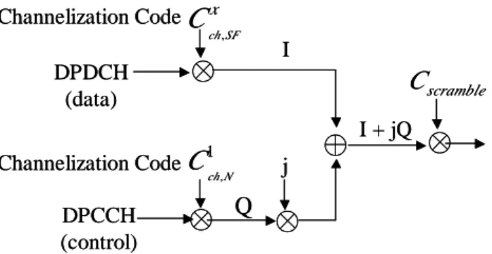
(2) approximate the reassignment based optimal solution. one N elements’ row vector. Then the generation method. concerned with blocking probability (BP). The BLRU. for the OVSF code-set is described as. algorithm needs neither code exchange nor reassignment. 1 Cch ,1 = 1,. process; therefore,. SC is decreased. At the same time,. we devise a compact data structure to store an OVSF code table and an unused-code list. It can save extra storage for. 1 1  C ch   C ch ,1 ,2  2  =  1  C ch , 2   C ch ,1. the unused code list and avoid search operation of the OVSF code tree. Additionally, an OVSF code generation function is designed to generate the corresponding codeword, instead of storing a real codeword straight in an array, to save about 89 percent of space. As a result, it is. C ch , N. especially suitable for mobile sets (MS). The rest of this paper is organized as follows. The OVSF code system is described in Section II. Section III illustrates a compact data structure and the BLRU code assignment algorithm. In order to realize the cost of the BLRU algorithm, Section IV evaluates its time and space. 1   1 1  C ch ,1  =   1 C ch  1 − 1  ,1 . C 1  1ch , N / 2 C  C 1ch , N   ch2 , N / 2  2   C ch , N / 2 C =  ch , N  =  C 2  ...   ch , N / 2  C N   ... N /2  ch , N   C ch , N / 2 C N / 2  ch , N / 2. C 1ch , N / 2   C 1ch , N / 2  C ch2 , N / 2   2 C ch , N / 2  ,  ...  C chN, /N2/ 2   C chN, /N2/ 2 . where C kch , N / 2 is the binary complement of C k . The ch , N / 2. complexity. Simulation results are shown in Section V.. vector C chk , N = (c1k , c 2k ,..., c Nk ) ∈ {±1} N can be called a. Finally, concluding remarks are given in Section VI.. codeword. If. C chk , N is used (assigned), other users. cannot use all ancestor codes of II.. OVSF Code System. The channelization operation in WCDMA transforms each data symbol into a number of chips. The number of. C chk , N and all. descendant codes generated from this code. Certainly, all codes of. C chk , N are orthogonal to each other.. chips per data symbol is called spreading factor. The. Furthermore, both the forward link (downlink) and the. channelizing structure of the reverse link (uplink) in the. reverse link in WCDMA can apply OVSF code(s) to. OVSF code system is shown in Figure 1. The data. match the request data rate. Without loss of generality, the. symbols are spread in channelization operation firstly and. data rate described in this paper is normalized by the basic. then scrambled in scrambling operation [4].. data rate Rb of an OVSF code with the maximum spreading factor (MaxSF). We assume that MaxSF = 256. Channelization Code C x. ch , SF. DPDCH (data). ⊕ 1. Channelization Code C ch , N DPCCH (control). here.. I. C 1ch , 4 = {1,1,1,1}. C scramble j. ⊕. I + jQ. C 1ch , 2 = {1,1}. ⊕. C ch2 , 4 = {1,1,−1,−1} C 1ch ,1 = {1}. ⊕ Q ⊕. C ch3 , 4 = {1,−1,1,−1} C ch , 2 = {1,−1} 2. Figure 1: Channelizing structure of the reverse link in the OVSF code system. C ch , 4 = {1,−1,−1,1} 4. In channelization operation, a code tree shown in. C 1ch ,8 C ch2 ,8 C ch3 ,8 C ch4 ,8 C ch5 ,8 C ch6 ,8 C ch7 ,8 C 8ch ,8. Figure 2 recursively generates the OVSF codes based on a. SF=1. modified Walsh-Hadamard transformation [4]. For example, Cchk , N uniquely describes the codes, where N is. Figure 2: Code tree for generation of the OVSF codes. the spreading factor of the code, k is the code number, and 1≤k≤N. Let Cch, N denote the set of N binary OVSF codes {C. k N ch , N k =1. }. , where N=2n ranges from 4 to 256 and C. k ch , N. is. SF=2. SF=4. SF=8. Actually, the number of the OVSF codes is limited. The base station (BS) may therefore run out of the codes and block an incoming call. Four issues affecting the BP.

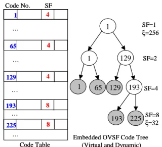
(3) of the OVSF code system are stated in the following. The. extra storage for the list and avoid searching the code tree.. first is how much bandwidth the system can provide. An. The primary structure of a code entry in an OVSF code. overloaded system blocks incoming calls more frequently.. table implemented by a 2D array is shown in Figure 4.. The second is the arrival rate (calls per unit time) and the. Field Code No. (e.g., n) is the index to the nth code entry.. incoming call-duration. High arrival rate and long. Shaded Codeword is a binary sequence that represents an. call-duration may dramatically increase the system load.. OVSF code by taking its prefix SF bits. This field is not. The third is the variable request data rate. An incoming. required if the Decimal Walsh Code Generating Function. call is blocked if the available codes in BS are not enough. (DWCGF, will be illustrated in Section IV) is further. to fulfill the request. The fourth is the grade of OVSF. applied. The Used Flag field is set to “false” initially and. code-set fragmentation. After a sequence of code. is changed to “true” as the codeword in the same entry is. assignment and release operations, the OVSF code tree. assigned. Field SF stores the current spreading factor. consists of many fragmental nodes. This fragmentation. possessed by a code entry. Both fields PREV and NEXT. will degrade the performance of the code assignment. For. are used for the unused (available) OVSF code list shown. example, as shown in Figure 3, a new call requesting a. in Figure 6. Given a code entry in the unused code list,. C. x ch , 2. , which cannot be supported, will be. field NEXT points to its successor, and field PREV points. blocked although the system has enough overall capacity. to its predecessor. The unused code list is therefore. single code. (the aggregation of the code. C. 3 ch , 4. C. ,. 1 ch , 8 ,. and. C. 8 ch , 8. equals to. C chx , 2 ). This is called “fragmentation,” which. results in less code assignment flexibility and higher BP. A dynamic assignment approach in [3] can gather the. embedded in the code table; that is, we do not need any other additional memory to store the list. Moreover, the code table embeds the OVSF code tree, all codeword entries, and used code records.. available codes together dynamically so as to provide. Code No.. more flexibility by exchanging them. One disadvantage of. 8 bits. the approach is the increased SC, because it needs to deal with the code exchange and reassignment processes. 1 Cch ,8. C. Cch2 ,8 C. C C. Cch3 , 4 C. 1. 4 ch ,8. Cch5 ,8. 2 ch , 2. C. 4 ch , 4. SF=1 ξ=256. 1. Blocked code. 65. 4. 1. … Assigned code. 129. 8 ch ,8. Figure 3: An example of OVSF call blocking due to fragmentation. Best-fit Least Recently Used Algor ithm. To achieve less fragmentation and complexity, we propose an efficient BLRU code assignment algorithm.. 129. SF=2. 42. 1. …. C. III.. SF 41. …. Cch6 ,8 Cch7 ,8. SF: spreading factor PREV: the pointer to its predecessor NEXT: the pointer to its successor. Code No.. 2 ch , 4. 1 Cch ,1. 1 bit 8 bits 8 bits 8 bits. 256 bits. Available code. 3 ch ,8. C. PREV NEXT. Figure 4: The primary structure of a code entry in an OVSF code table. 1 ch , 4. 1 ch , 2. Used SF Flag. Code word word Codewor d. 193 …. 84. 225 …. 8 Code Table. 65 129. 193. 193 SF=4. 225. SF=8 ξ=32. Embedded OVSF Code Tree (Virtual and Dynamic). Figure 5: An example presents that the code table embeds the OVSF tree. Firstly, a compact data structure is devised to store the. An example of the embedded OVSF code tree can be. OVSF code table and the unused code list. It can save. seen in Figure 5. For each code i, its dynamic left child.

(4) code is code no. i and right child code is code no. i +. the prefix MaxSF /ξ bits of the codeword indexed by. MaxSF /2*SF. When a user requires a code with SF=8, Code 193 (SF = 4) needs to be split into two codes:Code 193 and Code 225, with SF = 8. The value of field SF of each code entry is dynamically changed according to the current status. When Code 1 and Code 65 with SF = 4 are released, these two codes should be merged into Code 1 with SF = 2. Thus, the code table simultaneously maintains the OVSF code tree. Meanwhile, this code table requires only 256 code entries and saves 255 nodes and 254 links in a real OVSF code tree. Figure 6 demonstrates the unused code list organized by a logical double-linked list and ordered by the spreading factor. In fact, the list is embedded in the code table as described above. Besides pointers PREV and NEXT in each code entry, the code table requires some other pointers. Pointer Head points to the first element of the list, pointer Tail points to the last element of the list, and other log2(MaxSF ) + 1 pointers (namely, SFpointer[x], 0≤x≤8 if MaxSF = 256) let the BLRU algorithm directly index into the best-fit code entries. The unused code list needs only to link those code entries which are the roots of unused code sub-trees. For example, as shown in Figure 3,. SFpointer[log2(ξ)] if the index is not NULL and MaxSF /ξ. only. 1 8 C ch3 , 4 , C ch , 8 , and C ch , 8 codes have to be linked. in the list, but not. C ch5 ,8 or C ch6 ,8 .. SFpointer[0]. Head. SFpointer[1]. SFpointer[log2ξ] (Front). Assignment (The Best-fit entry). }. equals to the field SF. That is the best-fit strategy. Perhaps none of the unused codes has the same spreading factor to. MaxSF /ξ, the code has to be split if the field SF is greater than MaxSF /ξ. Otherwise, the call is blocked if the pointer index is NULL. This best-fit strategy in the BLRU algorithm is the most straightforward one to select an unused code from the set of available codes. It always chooses the code with the best spreading factor first. In static code assignment, assigning a code at random certainly results in a lot of fragmental codes. In dynamic code assignment, as described in [3], the optimal dynamic code assignment algorithm alternatively suffers from the additional overhead of code exchange and reassignment, although the overhead is minimized as much as possible. This overhead increases the SC dramatically, in a software and/or hardware. Intuitively, a good approximation to the optimal solution is based on the observation that codes assigned first will have a higher probability to be released first. The popular least recently used (LRU) algorithm is considered to have an adequate performance. It tends to minimize the number of fragmental codes. In our BLRU algorithm, searching for a LRU code is not required since the corresponding SFpointer points to the front of the best-fit entries and each entry group with the same spreading factor is a natural LRU queue. Of course, timestamps or time counters are not required either. The brief flowchart of the BLRU algorithm is plotted in Figure 7 and the algorithm is shown as follows.. SF =MaxSF/ξ. SFpointer[log2ξ + 1] (Rear). Release (Natural LRU queueing). SFpointer[log2MaxSF] Tail. Figure 6: The unused OVSF code list organized by a logical double-linked list A data rate Ri for call i is a multiplication of the basic transmission rate Rb, where 1 (spreading factor = 256) ≤ Ri ≤ 64 (spreading factor = 4). Then calculate Ri’s approximate single-code rate ξ ( Ri ) = 2 log 2 ( 2*Ri −1)  . Subsequently, user admitted code can be represented by. BLRU code assignment algorithm Input: A request data rate Ri for call i Output: An allocated code number Ni if call accepted or a Null code number if call blocked. Step 1: > Calculate the approximate single-code rate ξ which is slightly higher than Ri. Formula: ξ ( Ri ) ← 2 log 2 ( 2*Ri −1) . Step 2:. MaxSF ← Maximum spreading factor > Check if the code rate ξ is greater than the remaining available rates in system. If so, this call will be blocked. If ξ > (MaxSF – UsedDataRates) then goto Step 8. Step 3: > Check if there exists a code with SF ≥ MaxSF /ξ. If not, this call will be blocked..

(5) If SFpointer[log2 ξ].SF = NULL then goto Step 8. Step 4: > Best-fit strategy SFpointer[log2 ξ].CodeNo is the best-fit choice If SFpointer[log2 ξ].SF = MaxSF /ξ then goto Step 6. Step 5: > Code Splitting CSF ← SFpointer[log2 ξ].SF while (CSF > MaxSF /ξ) Split one code with spreading factor CSF into two codes with spreading factor CSF/2. CSF ← CSF/2. Modify SFpointer[log2 ξ] and some codes’ fields PREV and NEXT.. IV.. Complexity Analysis. To analyze the time complexity of the code assignment operation, all the steps in the BLRU algorithm are considered. Each step needs to execute only one time from Step 1 to Step 4. So do those steps from Step 7 to Step 9. In Step 6, the retrieve operation runs in O(1) time since at most some pointers must be modified for the unused code list. Only in Step 5, to split a code, the WHILE loop needs running k times, where k is no more than log2(MaxSF ). Therefore, the time complexity of the assignment part can be illustrated as T(k) = k + O(1) ≤ log2(MaxSF ) + O(1) > if MaxSF = 256. = 8 + O(1),. Step 6: > LRU code assignment Retrieve the front element of the entry group with spreading factor MaxSF /ξ. Ni ← SFpointer[log2 ξ].CodeNo > On the contrary, the code will be inserted into the rear position of the entry group with spreading factor MaxSF /ξ as a code is released. Step 7:. = O(1). Similarity, with according to the code release operation of the BLRU algorithm, all steps take O(1) time except for the codes merging step. For codes merging, the WHILE loop has to run m times. Hence, the time complexity of the release part can be represented by T(m) = m + O(1) ≤ log2(MaxSF ) + O(1). > Call accepted Code No. ← Ni goto Step 9. > if MaxSF = 256. = 8 + O(1), = O(1).. Step 8:. Totally, the BLRU algorithm takes only constant time > Call blocked Code No. ← NULL. in the worst case. Neither any dynamic code exchange and reassignment nor the code searching operation is required.. Step 9:. On the other hand, an OVSF code generation. Return. function – DWCGF -- is designed to generate the Start. corresponding codeword, instead of storing a real codeword straight in an array. Given a code number (index). Call setup Request rate ξ. Ni, DWCGF δ(SF, γ) is an efficient and correct code generating function that can save about 89 percent of. No. ξ≤ Available Capacity? Yes. Use BLRU Algorithm to decide admitting this call. No. Can BLRU allocate a code with SF=MaxSF/ξ ? Yes. BLRU Algorithm allocates the code for this call. space. How the DWCGF works is described as follows. The data rate Ri for call i can be assigned an approximate single-code rate ξ defined by. ξ ( Ri ) = 2 log. 2 ( 2* Ri −1). . .. Assume that code number Ni, an index of a code entry, is assigned. Let us define that ( N i − 1) ( N i − 1) N + ξ −1 γ = +1 = +1 = i. MaxSF SF. ξ. ξ. , where 1≤ γ ≤SF, γ∈N. Following the data-structure rule described as above, (Ni-1) must be the multiplication of ξ and the codes from Ni to Ni+ξ-1 will not be used. From. Block this call. Accept this call. Figure 7: A brief flow chart of the BLRU algorithm.. the point of view on the code tree, the codes from Ni+1 to Ni+ξ-1 are the descendants of the code Ni. Simultaneously, the used flag associated with the code Ni turns to “true.” If each code entry consists of a real codeword (256 bits) in.

(6) the code table, the prefix SF bits of the codeword are. Table 1: Examples of OVSF code generation via DWCGF. fetched directly. Alternatively, the DWCGF formula can. Walsh code. OVSF code. derive the codeword with spreading factor SF in only O(1). SF CGF. running time. The DWCGF formula is shown by. 1 δ(1,1). 00. (1). C1,1. 2 δ(2,1). 0 00. (1,1). C2,1. δ(2,2). 1 01. (1,-1). C2,2. 4 δ(4,1). 0 0000. (1,1,1,1). C4,1. δ(4,2). 3 0011. (1,1,-1,-1). C4,2. δ(4,3). 5 0101. (1,-1,1,-1). C4,3. sequence of binary digits and retrieve the least significant. δ(4,4). 6 0110. (1,-1,-1,1). C4,4. SF bits. With digit 0 represents +1 and digit 1. 8 δ(8,1). δ(1, 1) = 0.. SF δ ( SF , γ ) = δ ( SF , γ  ) * ( 2 + 1) + [(γ − 1) mod 2] 2  2 SF *[ 2 − 1 − 2 * δ ( SF , γ )]. 2  2 Next, we translate the decimal value of δ(SF, γ) to a. Value. SF bits. Code word. Code. 0 00000000 (1,1,1,1,1,1,1,1). C8,1. δ(8,2). 15 00001111. (1,1,1,1,-1,-1,-1,-1) C8,2. Examples of the OVSF code generation via DWCGF. δ(8,3). 51 00110011. (1,1,-1,-1,1,1,-1,-1) C8,3. are shown in Table 1. The boundary condition of δ(SF, γ). δ(8,4). 60 00111100. (1,1,-1,-1,-1,-1,1,1) C8,4. is that δ(1, 1) = 0. By DWCGF and the table index Ni, BS. δ(8,5). 85 01010101 (1,-1,1,-1,1,-1,1,-1) C8,5. can obtain any OVSF codeword with at most log2(MaxSF ). δ(8,6). 90 01011010 (1,-1,1,-1,-1,1,-1,1) C8,6. times recursively.. δ(8,7). 102 01100110. δ(8,8). 105 01101001 (1,-1,-1,1,-1,1,1,-1) C8,8. represents –1, this maps the result to an OVSF code.. Let n = spreading factor. The time complexity of. (1,-1,-1,1,1,-1,-1,1) C8,7. function δ(SF, γ) can therefore be described by the V.. recurrence T(n) = T(n/2) + O(1),. Simulation Results. Three approaches, namely, the random, the BLRU, and. where T(1) = O(1) is the boundary case.. the. By iteration method,. algorithms, are simulated here for comparison. With. T(n) ≤ T(MaxSF ). > in the worst case. reassignment. based. optimal. code. assignment. respect to the code-limited system, the total BP represents. = T(MaxSF/2) + O(1). the performance of the channelization code assignment. = (T(MaxSF/4) + O(1)) + O(1). algorithm. In case of approximate single code, the BS will. =…. assign only one code whose rate is slightly higher than the. = T(1) + log2(MaxSF ) * O(1). requested. Request data rate is normalized to 2n style.. = O(1) + log2(MaxSF ) * O(1). These simulations use the following parameters as in [3].. = 9 * O(1),. > if MaxSF = 256. l. λ = 4-64 calls/unit time.. = O(1) Thus, the DWCGF function also performs only in constant. Call arrival process is Poisson with mean arrival rate. l. time.. Call duration is exponentially distributed with a mean value of 1/µ = 0.25 unit of time.. To analyze the space requirement, we do not require. l. Maximum spreading factor = 256.. the real OVSF code tree and the unused code list. And,. l. Capacity test: code-limited.. each code entry in Figure 4 without the codeword part. In addition,. requires only 33 bits when DWCGF is used. An. l. Rmax denotes the maximum request data rate. implemented OVSF code table with 256 entries plus. l. Rmean denotes the mean request data rate. eleven additional pointers requires only about 1K bytes of. The simulations employ two types of request. memory. On the contrary, if DWCGF is absent, the code. rate-source models: a uniform distribution and an. table requires about 9K bytes of memory. In brief, applying the function DWCGF can save further 89 percent. exponential one. The uniform simulation generates the request rate Ri distributed uniformly with the mean rate =. of space. This alternative is especially feasible and. Rmean and the maximum rate = Rmax for call i. Figures 8 to. suitable for the MSs with a very small memory size.. 10 show the results with uniform rate-distribution, where Rmean and Rmax is up to 32Rb and 64Rb, respectively. The.

(7) mean arrival rate λ ranging from 4 to 64 calls per unit time. algorithm needs neither code exchange nor reassignment. is represented on the horizontal axis. And the average BP. process is notably mentioned, although the optimal case. for a long period of time is indicated on the vertical axis.. slightly outperform it. 50%. From the three figures, the optimal solution has the lowest. one.. Figure 8 represents the typical case and the. practical operational region. Generally, the BLRU algorithm is always superior to the random case.. Maximum available data rate = 64Rb. 35% 30% 25% 20% 15% 10%. 3.5%. 5%. 3.0%. 0%. Requested data rate distributed uniformly With mean = 8Rb. 2.5% Blocking probability. With mean = 32Rb. 40% Blocking probability. optimal solution; the random approach usually is the worst. Requested data rate distributed uniformly. 45%. BP almost always. The BLRU algorithm is close to the. 4. 8. 12. 16. Maximum available data rate = 16Rb. 20 24 28 32 Mean arrival rate (calls/unit time) Optimal. BLRU. 36. 40. 44. 48. Random. 2.0% 1.5%. Figure 10: Comparison among three different algorithms using uniform rate distribution with Rmean = 32Rb and Rmax = 64Rb.. 1.0% 0.5% 0.0%. 18.0%. 16. 20. 24. 28. 32. 36. 40. 44. 48. 52. 56. 60. 64 16.0%. Mean arrival rate (calls/unit time) BLRU. Requested data rate distributed exponentially With mean = 16Rb. 14.0%. Random. Figure 8: Comparison among three different algorithms using uniform rate distribution with Rmean = 8Rb and Rmax = 16Rb.. 12.0% Blocking probability. Optimal. Maximum available data rate = 32Rb. 10.0% 8.0% 6.0% 4.0% 2.0%. 35% 0.0%. Requested data rate distributed uniformly. 30%. 4. Blocking probability. With mean = 16Rb 25%. 8. 12. 16. 20. 24 28 32 36 40 44 Mean arrival rate (calls/unit time) Optimal. Maximum available data rate = 32Rb. BLRU. 48. 52. 56. 60. 64. Random. 20%. Figure 11: Comparison among three different algorithms using exponential rate distribution with Rmean = 16Rb and Rmax = 32Rb.. 15% 10% 5% 0% 4. 8. 12. 16. 20. 24. 28. 32. 36. 40. 44. 48. 52. 56. 60. 64. Mean arrival rate (calls/unit time) Optimal B. BLRUB. Random. om. Figure 9: Comparison among three different algorithms using uniform rate distribution with Rmean = 16Rb and Rmax = 32Rb.. On the other hand, the exponential simulation generates the request rate Ri distributed exponentially for call i. The results in Figures 11 to 12 with exponential rate-distribution are similar to those described above, except for an interesting region. The interesting region is on the right upper corner in Figure 12, where the mean arrival rate ranges from 50 to 64. In the region, the BLRU. Figure 9 shows the case that Rmean = 16Rb and Rmax =. algorithm outperforms the optimal case. The reason is that. 32Rb. As the maximum request data rate grows, the BPs of. the fragmentation with a moderate number of fragmental. all approaches increase and the BLRU solution is getting. codes has more total call accepted times in the BLRU case. closer to the optimal case. For the case shown in Figure 10,. rather than those in the optimal case, when both the arrival. the three lines behave almost closely. The heavy traffic. rate and the request data rate are high enough. However,. causes the system to move beyond the practical region. In. this is only a phenomenon but not in practical working. practical region, the BP needs smaller than 5 to 10 percent. area. High BP caused by high arrival rate and high request. generally. Consequently, we can conclude that the BLRU. rate has to be decreased by increasing the system capacity,. algorithm performs a well result. And, that the BLRU. e.g., more micro-cells established. As a result, if we take.

(8) both the BP and the SC issues into account, the BLRU algorithm is a better approach. 25%. Requested data rate distributed exponentially With mean = 16Rb. Blocking probability. 20%. Maximum available data rate = 64Rb 15%. 10%. 5%. 0% 4. 8. 12. 16. 20. 24 28 32 36 40 44 Mean arrival rate (calls/unit time). m o. Optimal. BLRU. 48. 52. 56. 60. 64. Rand. Figure 12: Comparison among three different algorithms using exponential rate distribution with Rmean = 16Rb and Rmax = 64Rb. VI.. Conclusions. Some OVSF code assignment methods for variable rate transmission have been investigated in the literature. Both single code and multicode assignment algorithms suffer from fragmentation problem, which degrades the performance of the code assignment. In this paper, we proposed to use the Best-fit Least Recently Used (BLRU) algorithm to resolve the performance issue.. In addition, two different approaches. were simulated and compared to the BLRU algorithm in terms of Blocking Probability. As a consequence, considering both the Blocking Probability and System Complexity, , the BLRU algorithm is a very suitable algorithm for the channelization code assignment in 3G WCDMA.. References 1. A. J. Viterbi, CDMA: Principles of Spread Spectrum 2.. 3.. 4.. 5.. Communications, Addison-Wesley, 1995. R. Kohno, R. Meidan, and B. Milstain, “Spread spectrum access methods for wireless communications,” IEEE Commun. Mag., vol. 33, pp. 58-67, Jan. 1995. T. Minn and K.-Y. Siu, “Dynamic Assignment of Orthogonal Variable-Spreading- Factor Codes in W-CDMA,” IEEE Journal on Selected Areas in Commun., vol. 18, no. 8, pp.1429-1440, August 2000. 3GPP Technical Specification 25.213, v3.3.0, Spreading and modulation (FDD) (Released in 1999), June 2000. I. Chih-Lin and R. D. Gitlin, “Multi-code CDMA. Wireless Personal Communications Networks,” in. Proc. of ICC’95, pp. 1060-1064, June 1995. 6. T. Ottosson and T. Palenius, “The Impact of Using Multicode Transmission in the WCDMA System,” in Proc. of IEEE VTC’99, vol. 2, pp. 1550-1554, May 1999. 7. F. Adachi, K. Ohno, A. Higashi, T. Dohi, and Y. Okumura, “Coherent Multicode DS-CDMA Mobile Radio Access,” IEICE Trans. Commun., vol.E79-B, no.9, pp.1316-1325, Sept. 1996. 8. Harri Holma and Antti Toskala, WCDMA for UMTS, John Wiley & Sons, 2000. 9. E. Dahlman and K. Jamal, “Wide-band Services in a DS-CDMA Based FPLMTS System,” in Proc. of the 46th IEEE VTC’96, pp.1656-1660, Atlanta, April 1996. 10. S. Ramakrishna and J. M. Holtzman, “A Comparison between Single Code and Multiple Code Transmission Schemes in a CDMA System,” in Proc. of the 48th IEEE VTC’98, pp.791-795, May 1998. 11. S. J. Lee, H. W. Lee, and D. K. Sung, “Capacities of Single-Code and Multicode DS-CDMA Systems Accommodating Multiclass Services,” IEEE Trans. On Vehicular Tech., vol. 48, no. 2, pp.376-384, March 1999. 12. P. Agin and F. Gourgue, “Comparison between Multicode with Fixed Spreading and Single Code with Variable Spreading Options in UTRA/TDD,” in Proc. of the 2nd IEEE SPAWC'99, pp.325-328, May 1999..

(9)