運用決策樹於腦部核磁共振影像之監督式腦組織分割研究

全文

(1) . 國立交通大學電機與控制工程學系博士論文. 運用決策樹於腦部核磁共振影像之監督式腦組織分割研究. A Supervised Segmentation of Brain MRI Tissue Using Decision Trees. 研究生：趙文鴻指導教授：陳右穎. 博士. 中華民國九十七年九月. .

(2) . 運用決策樹於腦部核磁共振影像之監督式腦組織分割研究. A Supervised Segmentation of Brain MRI Tissue Using Decision Trees. Student：Wen-Hung Chao. 研究生：趙文鴻指導教授：陳右穎博士. Advisor：Dr. You-Yin Chen. 國立交通大學電機與控制工程學系博士論文. A Dissertation Submitted to Department of Electrical and Control Engineering College of Electrical Engineering National Chiao Tung University in partial Fulfillment of the Requirements for the Degree of Doctor of Philosophy in Electrical and Control Engineering September 2008 Hsinchu, Taiwan, Republic of China. 中華民國九十七年九月. .

(3) . 運用決策樹於腦部核磁共振影像之監督式腦組織分割研究. 學生：趙文鴻. 指導教授：陳右穎. 國立交通大學電機與控制工程學系. 摘. 博士. 博士班. 要. 本文研究之目的主要是運用決策樹以增進腦部核磁共振影像於組織分割的準確度達到一個高品質的腦部組織分割為目標，首先，此研究提出用一個多階層仿視覺 (Multiscale retinex) 演算法來校準核磁共振影像之不均勻度 (Inhomogeneity)，此實驗之核磁共振影像含有假體核磁共振影像與老鼠之腦部核磁共振影像，經此演算法校準後可獲得較好的影像品質與清清晰的深層腦部結構影像，此外也用訊號峰值對雜訊比 (Peak-signal-to-noise) 與 (Contrast-to-noise) 對比度對雜訊比來評估校準後的影像品質。進一步實驗為得到腦部不同組織解剖結構，我們提出用分類與迴歸決策樹 (CART) 來分割模擬之假體核磁共振影像與模擬之腦部核磁共振影像，進行組織分割實驗後得到良好的腦部解剖組織影像。接下來更進一步實驗為增加腦部組織分割的準確度以提供神經解剖應用性，我們提出用一個促進式之決策樹 (Boosted decision tree) 分割模擬之假體核磁共振影像與模擬之腦部核磁共振影像與人體實體之腦部核磁共振影像，進行組織分割實驗後得到更準確之腦部解剖組織影像。以上兩個實驗之分割結果並且都用準確率 (Accuracy rate) 與 k 指標 (k index) 來量化評估其影像分割之表現。最後一個實驗是要得到腦部核磁共振影像之高品質分割影像，我們提出用一個促進式之決策樹為基礎結合以一個多階層仿視覺演算法為影像前處理之不均勻度校準分析，接著用促進式之決策樹來分割模擬之腦部核磁共振影像進行組織分割，除了能成功地對模擬之腦部核磁共振影像進行組織分割之外，經實驗分析後得到非常準確之腦部解剖組織影像，大大地改善了核磁共振影像之不均勻度與雜訊對影像分割之準確度所造成之影響，更加提高了組織分割的準確率，最後結果得到高品質的腦部組織分割，結果將對於腦部神經解剖之應用性有很大的幫助。 i .

(4) . A Supervised Segmentation of Brain MRI Tissue Using Decision Trees Student：Wen-Hung Chao. Advisor：Dr. You-Yin Chen. Department of Electrical and Control Engineering National Chiao Tung University. ABSTRACT. The purpose of this research is to achieve the high quality of brain tissue segmentation by using decision trees from magnetic resonance (MR) images. First, we proposed a multiscale retinex algorithm to correct the intensity inhomogeneity of brain MR images which include phantom data and animal data to obtain better image quality and clearer deep brain structures. The intensity inhomogeneity often occurs in MR images which are received by surface coils. The peak-signal-to noise (PSNR) and contrast-to- noise (CNR) were both used to evaluate the correction performance. Second, we used a classification and regression tree (CART) to segment brain MR images, including simulated phantom MR (SPMR) images and simulated brain MR (SBMR) images, to successfully segment brain tissues. Third, we proposed a boosted decision tree combined with fuzzy threshold to segment brain MR images, including SPMR images, SBMR images, and a real data, to achieve higher accuracy rate of brain tissue segmentation. The accuracy rate and k index were better when we used the boosted decision tree algorithm combined with a fuzzy threshold to classify gray matter (GM), white matter (WM), or cerebral-spinal fluid (CSF) in brain. Finally, we used the boosted decision tree through preprocessing procedure by the multiscle retinex algorithm to greatly improve the brain tissue segmentation from SBMR images. The accuracy rate was the best when we used the boosted decision tree algorithm combined with a multiscale retinex algorithm as a preprocessing procedure to classify GM, WM, or CSF in brain MR images.. ii .

(5) . The results shows that a boosted decision tree combined with preprocessing by the multiscale retinex algorithm can successfully improve the accuracy rate of MR brain tissue segmentation and can achieve a high quality of tissue segmentation in brain MR images.. iii .

(6) . 誌. 謝. 首先感謝我的指導教授陳右穎博士在我研究方面的細心指導，使我的研究得以完整與周詳呈現與實現，使我在研究方法、研究思維學習到很多，對我未來的研究幫助很大，也拓展我的研究視野。在口試階段，感謝所有口試委員提供寶貴之意見使本論文得以更完備呈現，也感謝實驗室的同學、學弟與學妹們的幫忙協助使我能順利完成最後口試過程。在工作上，感謝長官們與同事們的幫忙與支持，在生活上，感謝我摯愛的雙親與我的家人在生活方面的支持、包容與鼓勵。博士班進修階段求學歷程總會遇到許多的困難與挫折，然而除了需要體力以外更需要有健康與正向的想法與心態來面對這一切過程，我感謝我的師父太極門掌門人洪道子博士 (www.taijimen.org) 收我為徒，我的師父教導我如何練好身體培養好體力、涵養武德與修改心性使我能夠以一個學習與感恩的心來接受這所有的經歷，也感謝太極門師兄師姊們真誠的關心與鼓勵，這一切使我在心情起伏時調適自己的精神良方，面臨事情能歡喜以對。於此，謹以此論文獻給我的師父、師母、我的父親、母親、師兄師姊、我的師長、我所有的家人與朋友，感謝你們。 .. iv .

(7) . Contents Chapter 1 Introduction .................................................................................... 1 1.1.. The overview of the megnetic resonance imaging ..................................................... 1. 1.2.. Brain MR image quality and segmentation problem .................................................. 5. 1.3.. Literature reviews ....................................................................................................... 5. 1.3.1. Reviews of the MR image inhomogeneity correction approaches....................................................... 6 1.3.2. Reviews of the brain MR image segmentation approaches ................................................................. 7 1.3.3. Reviews of the MR brain image inhomogeneity correction prior to segmentation ............................. 9. 1.4.. Motivations ............................................................................................................... 11. 1.5.. The goals of this research ......................................................................................... 12. 1.6.. The main contributions ............................................................................................. 13. 1.7.. The organization of this dissertation ........................................................................ 15. Chapter 2 Correction of Inhomogeneous MR Images Using Multiscale Retinex (MSR)................................................................................... ........................................................................................................ 16 2.1.. Introduction .............................................................................................................. 16. 2.2.. Materials and methods .............................................................................................. 17. 2.2.1. Retinex algorithm .............................................................................................................................. 17 2.2.2. Single-scale retinex............................................................................................................................ 18 2.2.3. The surround function........................................................................................................................ 19 2.2.4. Adjustment of single-scale retinex output ......................................................................................... 20 2.2.5. Multiscale retinex .............................................................................................................................. 22 2.2.6. Phantom and animal magnetic resonance imaging ............................................................................ 23 2.2.7. Peak signal-to-noise ratio and contrast-to-noise ratio analysis .......................................................... 24. 2.3.. Experimental results ................................................................................................. 25. 2.3.1. Results of phantom image ................................................................................................................. 25. v .

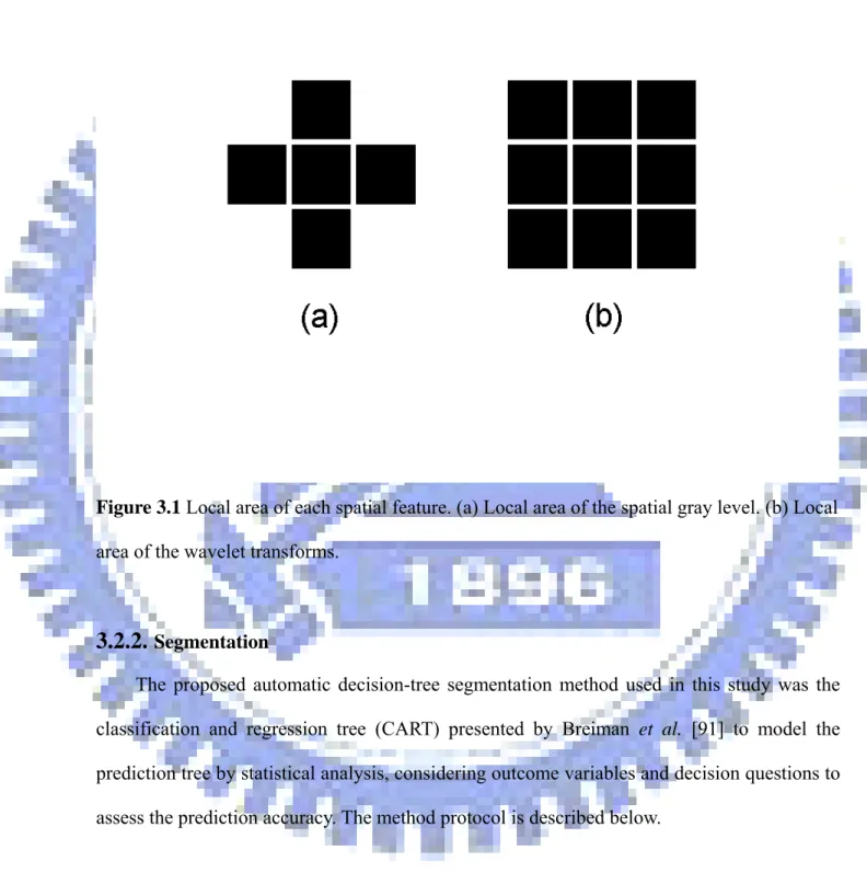
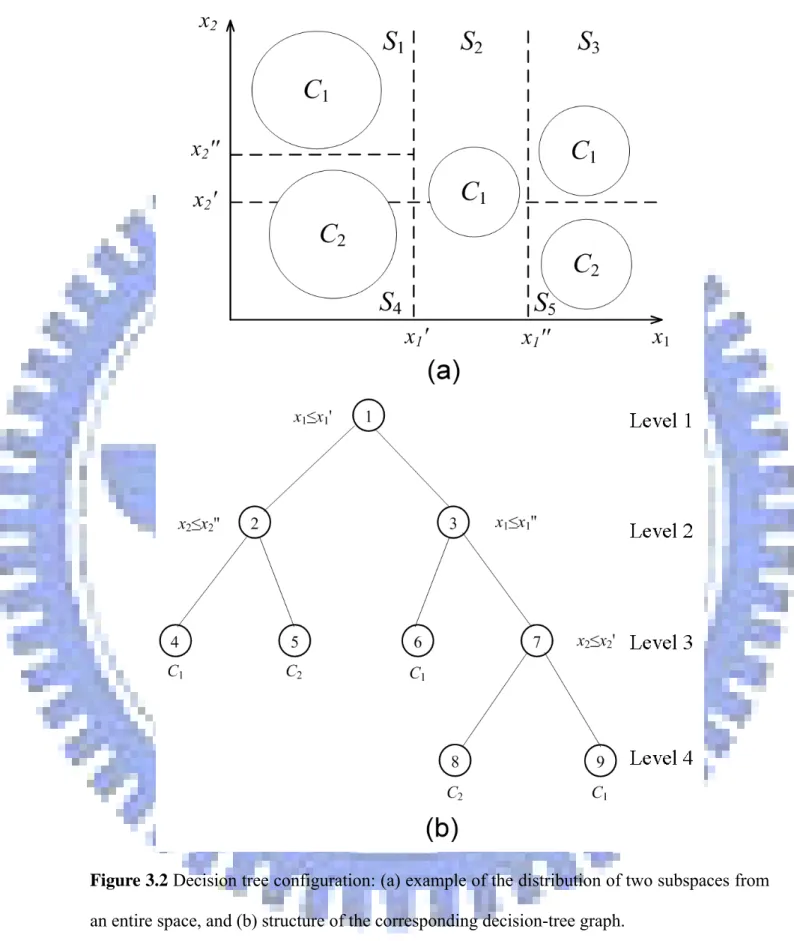
(8) 2.3.2. Results of animal image..................................................................................................................... 27 2.3.3. Comparisons of histogram equalization, local histogram equalization, and a wavelet-based algorithm with multiscale retinex .................................................................................................................................. 30 2.3.4. Results of peak signal-to-noise ratio and contrast-to-noise ratio analysis ......................................... 34. 2.4.. Discussions ............................................................................................................... 38. Chapter 3 Segmentation of Brain MR Images Using a Classification and Regression Tree (CART) ........................................................... 40 3.1.. Introduction .............................................................................................................. 40. 3.2.. Materials and methods .............................................................................................. 41. 3.2.1. Image preprocessing .......................................................................................................................... 41 3.2.2. Segmentation. .................................................................................................................................... 43 3.2.3. Decision tree classification ................................................................................................................ 43 3.2.4. Decision tree construction ................................................................................................................. 43 3.2.5. Simulated data. .................................................................................................................................. 43 3.2.6. Accuracy rate of segmentation. ......................................................................................................... 50. 3.3.. Experimental results ................................................................................................. 51. 3.3.1. Results of phantom image. ................................................................................................................ 51 3.3.2. Results of simulated brain MR image................................................................................................ 54. 3.4.. Discussions ............................................................................................................... 63. Chapter 4 Segmentation of Brain MR Images Using a Boosted Decision Tree (BDT) ........................................................................................ ........................................................................................................ 67 4.1.. Introduction .............................................................................................................. 67. 4.2.. Materials and methods .............................................................................................. 68. 4.2.1. MR data. ............................................................................................................................................ 68 4.2.2. Image preprocessing .......................................................................................................................... 69 4.2.3. Segmentation ..................................................................................................................................... 69 4.2.4. Decision tree classification ................................................................................................................ 70 vi .

(9) 4.2.5. Decision tree construction with gain ratio ......................................................................................... 71 4.2.6. Boosting ............................................................................................................................................. 72 4.2.7. Fuzzy threshold.................................................................................................................................. 74 4.2.8. Pruning .............................................................................................................................................. 74 4.2.9. Three-dimensional reconstruction ..................................................................................................... 75 4.2.10. The evaluation index of segmentation .............................................................................................. 75. 4.3.. Experimental results ................................................................................................. 76. 4.3.1. Segmentation of SPMR images ......................................................................................................... 76 4.3.2. Segmentation of SBMR images ......................................................................................................... 79 4.3.3. Comparison of segmentation with the other algorithms .................................................................... 84 4.3.4. Segmentation of real data in brain MR images .................................................................................. 88. 4.4.. Discussions ............................................................................................................... 91. Chapter 5 Improving Segmentation of Brain MR Images Based on a Boosted Decision Tree through Preprocessing by the Multiscale Retinex Algorithm ........................................................................ 96 5.1.. Introduction .............................................................................................................. 96. 5.2.. Materials and methods .............................................................................................. 96. 5.2.1. MR data in this experiment................................................................................................................ 96 5.3.2. Methods ............................................................................................................................................. 97. 5.3.. Experimental results ................................................................................................. 98. 5.3.1. Results of SBMR images ................................................................................................................... 98 5.3.2. Segmentation of SBMR images ....................................................................................................... 100. 5.4.. Discussions ............................................................................................................. 107. Chapter 6 The Summary and Future Works ............................................. 109 References ...................................................................................................... 111. vii .

(10) . List of Figure Figure 1.1. Three axes systems and the directions of magnetic field ( B0 , B1 , and M ) in MR imaging systems. . .............................................................................................................................................. 3. Figure 1.2 An example of MRI system. ............................................................................................................... 4 Figure 1.3. The whole image processing procedures of this research. ................................................................ 13. Figure 2.1 A histogram distribution plot that illustrated the gain and offset values of an MR image. . ............. 21 Figure 2.2. Corrected MR images of a phantom demonstrating the performance of retinex............................... 26. Figure 2.3 Performance of the retinex was demonstrated with adjusted MR images of a coronal section of the rat brain. ........................................................................................................................................... 29 Figure 2.4. Corrected MR images of a phantom, obtained via four methods. ..................................................... 32. Figure 2.5. Corrected MR images of a rat brain obtained from four algorithms. ................................................ 34. Figure 3.1. Local area of each spatial feature. ..................................................................................................... 43. Figure 3.2 Decision tree configuration. .............................................................................................................. 46 Figure 3.3 Segmentation of phantom images from IBSR.. ................................................................................. 53 Figure 3.4 Average accuracy rates of segmentation obtained using a decision tree with different spatial information from original phantom images with different noise variations and inhomogeneities.. . 54 Figure 3.5. Results of segmentation using a decision tree for simulated MR images obtained from BrainWeb. 55. Figure 3.6 Average accuracy rates of segmentation with different spatial information from the original MR images with noise levels of T1n3, T1n5, T1n7, T1n9, and T1n15. .................................................. 56 Figure 3.7. Results of segmentation using a decision tree for simulated MR images. ........................................ 57. Figure 3.8 Average accuracy rates of segmentation with different spatial information from MR images with noise parameters of T1n3RF20, T1n5RF20, T1n7RF20, T1n9RF20, and T1n15RF20. .................. 58 Figure 3.9. Results of segmentation using a decision tree for simulated MR images. ........................................ 60. Figure 3.10 Average accuracy rates of segmentation with different spatial information from MR images with noise parameters of T1n3RF40, T1n5RF40, T1n7RF40, T1n9RF40, and T1n15RF40.. ................. 61 Figure 3.11 Accuracy rates of GM, WM, and CSF in simulated MR images segmented using a decision tree with spatial information (G, x, y, r, θ) for T1n3, T1n5, T1n7, T1n9, and T1n15 ............................. 62 Figure 4.1 A flow diagram of image processing procedures for MR image segmentation................................. 70 Figure 4.2 Schematic diagram of the decision tree structure. ............................................................................. 71 Figure 4.3 Accuracy rates of region segmentation obtained using different spatial features from simulated phantom MR images. ......................................................................................................................... 78 Figure 4.4 Images segmented from simulated phantom MR images with different spatial features and various noise and inhomogeneity levels. ........................................................................................................ 79 Figure 4.5. Mean accuracy rates of tissue segmentation from simulated brain MR images.. .............................. 81. Figure 4.6 Accuracy rates of tissue segmentation using a boosted decision tree algorithm on simulated brain MR images. ...................................................................................................................................... 82 Figure 4.7 Segmentation of simulated brain MR images from BrainWeb. ......................................................... 83 - viii -.

(11) Figure 4.8 A 3D reconstruction of segmented brain image data in axial view. .................................................. 84 Figure 4.9 Segmentation of real brain MR imaging data.................................................................................... 91 Figure 5.1 Image processing procedures in this experiment.. ............................................................................. 97 Figure 5.2 Average accuracy rates of all brain tissues segmented using BDT with spatial feature (G x, y, r, θ) and (S x, y, r, θ) for different boost trial numbers. ............................................................................. 99 Figure 5.3 Images from original, corrected using MSR, and segmented using BDT from SBMR with T1n3RF20 and T1n9RF40. .............................................................................................................. 100 Figure 5.4 Accuracy rates of tissue segmentation using a BDT algorithm on SBMR images with T1n3RF20, T1n5RF20, T1n7RF20, and T1n9RF20. .......................................................................................... 102 Figure 5.5 Accuracy rates of tissue segmentation using a BDT algorithm on SBMR images with T1n3RF40, T1n5RF40, T1n7RF40, and T1n9RF40. .......................................................................................... 105. - ix -.

(12) . List of Table Table 2.1 Comparisons of PSNR and CNR for phantom images obtained from retinex algorithms with those obtained from histogram equalization, local histogram equalization, and the wavelet-based algorithm. ........................................................................................................................................................... 36 Table 2.2 Comparisons of PSNR and CNR for animal images obtained from retinex algorithms with those obtained from histogram equalization, local histogram equalization, and the wavelet-based algorithm. ........................................................................................................................................................... 37 Table 3.1 Designations of the original phantom images obtained by combining the noise levels and inhomogeneities parameters. ............................................................................................................. 49 Table 3.2 Designations of the original simulated MR images obtained by combining the noise levels and inhomogeneities parameters. ............................................................................................................. 50 Table 4.1 Segmentation accuracy rates from SBMR images using the boosted decision tree, the SRG, and the AS algorithm...................................................................................................................................... 86 Table 4.2 The segmentation k indexes from SBMR images using the boosted decision tree, the SRG, and the AS algorithm...................................................................................................................................... 87 Table 4.3 Segmentation of MR images from two real subjects using the boosted decision tree, the SRG, and the AS method. ......................................................................................................................................... 90. -x-.

(13) . Chapter 1. Introduction. 1.1. The overview of the magnetic resonance imaging Magnetic resonance imaging (MRI) has been used to diagnose various diseases for a long time and represented an important diagnostic technique in medicine for the effective and noninvasive detection of objects such as cancers, tumors, edema, infarctions, organs, blood vessels, and brain tissues. MRI can also obtain soft anatomical tissues of high quality in medical image application. It has become a well-known medical image equipment and well-used technique in neurological diagnosis and clinical applications. The advantages of MRI are more obvious than other medical image equipments such as CT, ultrasound, and X-ray. Bloch et al. has discovered the phenomenon of nuclear magnetic resonance (NMR) through a nuclear induction experiment in 1946 [1–3]. Purcell et al. also independently discovered the NMR in liquids and in solids in 1946 [4]. Many discoveries and developments about NMR founded the MRI technique. Magnetic resonance (MR) image is constructed with the bases of the NMR phenomenon. The principles of NMR are described as below. In general, nuclei consist of protons and neutrons. In quantum mechanical property, the particles (electronics, protons, and neutrons) of atom rotates around their own axis and the rotating motion is called spin. The phenomena of spin exist in all the charged particles which are similar to small magnets. The magnetic dipole exists in all of the particles. The phenomenon of spin is more exhibited in nuclei with odd number of protons and neutrons. One of these is hydrogen. Hydrogen which has only one proton and is contained in water or fat can create the strongest magnetic moment. More than 63% of the human body is composed of water or fat. Thus, magnetic dipole variations of the hydrogen are widely applied in imaging for human body. In MRI procedure, the directions of magnetic field ( B0 , B1 , and M ) and three axes are -1-.

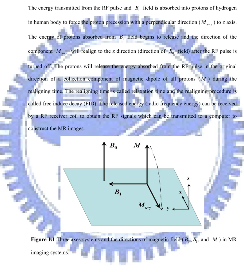
(14) . shown in Figure 1.1. Three axes are defined in MR imaging domain which are x axis (from back to front), y axis (from left arm to right arm), and z axis (from head to feet). The spin of proton in hydrogen can also create a tiny magnet. A collection of the magnetic dipole directions of spin of protons in hydrogen are arranged in the same direction of the magnetic field when all of them are located in a high external static magnet ( B0 ). The magnetic dipole directions of them are random orientations in the absence of an external magnetic field. The direction of the high external static magnet is usually called z direction (z axis). The units used to measure the strength of magnetic field are Tesla and gauss. An example to evaluate the magnetic strength is that the strength of the earth is 0.5 gauss. One Tesla equals to 10,000 gauss. The protons with spin axes in a high external static magnet also has precession phenomenon whose direction is parallel or anti-parallel to the magnetic field ( B0 ). The precession orientation which is a collection component ( M ) of magnetic dipole of all protons is around the magnetic field B0 . The precession phenomenon also exist frequency. The frequency of precession is called Larmor frequency which is the product of the gyromagnetic ratio and the magnetic field ( B0 ). The precession frequency is linearly proportional to the strength of the high external magnetic field ( B0 ). The gyromagnetic ratio of Hydrogen nucleus is 42.58 MHz/Tesla. Larmor frequency of hydrogen nucleus is 63.86 MHz when in a 1.5 Tesla of an external magnetic field ( B0 ). Larmor frequency of Hydrogen nucleus is 127.74 MHz when in a 3 Tesla of an external magnetic field ( B0 ). The precession direction of proton of hydrogen in human body is along z axis and its precession frequency also exists in a strong external magnetic field ( B0 ) for aligning the protons. In order to acquire the signals of magnetic dipole variations from hydrogen nuclei, the energy of a radio frequency (RF) pulse must be used to generate the signals and then the RF pulse coil transmitter will be turned off. When the same precession frequency of a RF pulse emits to protons, the nuclear magnetic resonance (NMR) phenomenon is generated. The -2-.

(15) . RF pulse is created from RF coils to construct a RF magnetic field (called B1 field). The strength of B1 field is smaller than that of external magnetic field ( B0 ) along the x-y plane. The energy transmitted from the RF pulse and B1 field is absorbed into protons of hydrogen in human body to force the proton precession with a perpendicular direction ( M x − y ) to z axis. The energy of protons absorbed from B1 field begins to release and the direction of the component M x − y will realign to the z direction (direction of B0 field) after the RF pulse is turned off. The protons will release the energy absorbed from the RF pulse in the original direction of a collection component of magnetic dipole of all protons ( M ) during the realigning time. The realigning time is called relaxation time and the realigning procedure is called free induce decay (FID). The released energy (radio frequency energy) can be received by a RF receiver coil to obtain the RF signals which can be transmitted to a computer to construct the MR images.. Figure 1.1 Three axes systems and the directions of magnetic field ( B0 , B1 , and M ) in MR imaging systems.. Two important parameters existing in FID procedure are T1 and T2. Two kinds of relaxation processes are: T1 relaxation time (longitudinal relaxation time) and T2 relaxation -3-.

(16) . time (transverse relaxation time). T1 relaxation time is the period while the protons release the energy absorbed from the RF pulse as heat to their surrounding environment (lattice) and the direction of a collection of magnetic dipole of all protons return to their equilibrium position (the original direction of component M , z direction, or longitudinal plane). T1 relaxation time is also called spin-lattice relaxation time. T2 relaxation time is the period while the protons release the energy absorbed from the RF pulse to their surrounding protons (spin) and the procedure causes a decrease in transverse magnetization ( M x − y in x-y plane) . T2 relaxation time is also called spin-spin relaxation time. Three types of MRI image are: T1-weighted image, T2-weighted image and PD-weighted image. T1-weighted image is constructed with the measurement of the T1 relaxation times for different tissues. T2-weighted image is obtained with calculation of the measured T2 relaxation times in different tissues. PD-weighted image which is the proton density image is acquired with the evaluation of the number of protons in a unit for different tissues. An example of MRI system is shown in Figure 1.2.. Figure 1.2 An example of MRI system (MRI/MRS Lab, National Taiwan University). -4-.

(17) . 1.2. Brain MR image quality and segmentation problem In this dissertation, we investigate some problems about MR image inhomogeneity and noise that might affect the image quality and decrease the accuracy of segmentation for diagnosis application. We address these problems to improve the brain MR image quality, to increase the segmentation accuracy of brain MR image, and to achieve the high quality of segmentation for brain MR anatomical structure. MR image intensities acquired from homogeneous tissue are often inhomogeneities due to bad radio frequency coil uniformity, gradient-driven eddy currents, and human anatomy both inside and outside the field of view. The noise existing in MR image also decreases the image quality due to the body movements, acquiring procedure, and receiver coils. Several factors make brain MR image segmentation difficult, including similar imaging intensities in different regions of the brain, overlapping intensity distributions, background noises, and radio-frequency (RF) inhomogeneities. The accuracy of segmenting the cortical surface for analyzing the volumes of different tissues such as gray matter (GM) and white matter (WM) significantly affects clinical diagnoses, but this is difficult to be achieved due to the presence of imaging noise and inhomogeneities. Furthermore, it is more difficult to improve the segmentation accuracy of brain MR image to achieve high quality of segmentation for anatomical structure.. 1.3. Literature reviews For MR image anatomical structure quality, the image intensity inhomogeneity and segmentation are two main problems. In this Section, we will review the literatures about inhomogeneity correction, segmentation approaches, and inhomogeneity correction prior to segmentation approaches for MR images.. -5-.

(18) . 1.3.1. Reviews of the MR image inhomogeneity correction approaches One of these factors is RF inhomogeneities of MR images. It often occurs in MR images obtained by receiving with surface coils during scanning on MR imaging. Several techniques were urged on improvements of surface coils to increase the MR image quality to help the clinical diagnosis [5–11]. It is more expensive to decrease effects of RF inhomogeneities by improving surface coils through the hardware technique. Therefore, an easy way through software methodology with low cost is helpful to decrease the effects of RF inhomogeneities. Many approaches have been recently proposed to correct MR image to improve the detection and diagnosis capabilities [12–20]. Haiguang et al. addressed the performances of enhancing hybrid MR images that were decreased by T2-weighted effects and measurement noise [11]. They reduce the imaging time using hybrid imaging sequences such that the T2 effects act as a distortion filter which will damage image quality and detection and which can be estimated and used in Wiener filter for global T2 amplitude restoration. The linear prediction was also used to predict the local signal and phase to estimate the frequency response of the T2 filter. These combined techniques successfully correct T2 distortion and reduce the measurement noise to demonstrate both phantoms and human data. Sled et al. corrected the MR image intensity inhomogeneity to achieve high performance without requiring a model of tissue classes present [13]. They used a nonparametric nonuniform intensity normalization to estimate both the multiplicative bias field and the distribution of true tissue intensity. They successfully corrected the simulated and real data to reduce intensity nonuniform and tissue intensity variation to obtain uniform image. The relative segmentation approaches are to correct the inhomogeneous image prior to the segmentation. Ahn et al. [14] proposed a method of local adaptive template filtering for enhancing the signal-to-noise ratio (SNR) in MRI without reducing the resolution. Moreover, Styner et al [15] showed that a parametric bias-field correction method could correct bias distortions that are much larger than the image contrast. Likar et al. [16] proposed a -6-.

(19) . model-based correction method to adjust inhomogeneity in the intensity of an MR image. They applied an inverse image-degradation model where parameters were optimized by minimizing the information content of simulated and real MR data. Lin et al. [17] used a wavelet-based algorithm to approximate surface-coil sensitivity profiles. They corrected image intensity in homogeneities acquired by surface coils, and used a parallel MRI method to verify the spatial sensitivity profile of surface coils from the images captured without using a body coil. It has also been shown [18, 19] that contrast enhancement can be used to improve the quality of MR images. More researches [20–25] were also urged to correct the RF inhomogeneity and to model bias field of MR images to improve the image quality. These proposed researches exhibit the importance of MR image inhomogeneity correction. In addition, the study of brain structure through MR image correction is very important for neurological applications. However, the correction of MR image intensity inhomogeneity is also a problem to improve the image quality with better visualization.. 1.3.2. Reviews of the brain MR image segmentation approaches Segmentation is one of the techniques used to classify the brain tissues in MR images, which is a basic problem for identifying anatomical structures in MR image processing. Several segmentation methods have been applied in the analysis of anatomical structures involving three-dimensional (3D) reconstruction, tissue-type contour definition, and clinical diagnosis [26, 27], and in cortical surface segmentation, volume assessment of brain tissue, tissue classification, tumor segmentation, and characterization of various brain diseases such as sclerosis, epilepsy, stroke, cancer, and Alzheimer’s disease [28, 29]. The accuracy of segmenting the cortical surface for analyzing the volumes of different tissues such as gray matter (GM) and white matter (WM) significantly affects clinical diagnoses, but this is difficult to be achieved due to the presence of imaging noise and inhomogeneities. Several segmentation techniques have been proposed for improving the detection of brain structures -7-.

(20) . in MR images in diagnostic and neuroanatomical applications. Both manual and automatic segmentation methods are used to segment brain MR images. Manual segmentation such as thresholding is a traditional method used to distinguish different tissues in MR brain images [30–32], but this is difficult in the presence of a low contrast-to-noise ratio, low signal-to-noise ratio (SNR), and overlapping of tissues in the gray-level distributions, and it is also very labor-intensive and time-consuming [33]. Therefore, several studies have investigated automatic segmentation methods for distinguishing brain MR images structures and improving the efficiency of segmentation and tissue classification [27, 34–41]. Marroquin. et al. presented an automatic segmentation method based on an accurate and efficient Bayesian algorithm [42]. Automatic segmentation based on a constrained Gaussian mixture model framework employed an expectation-maximization algorithm to determine parameters and segment both simulated and real three-dimensional, T1-weighted noisy MR images [43]. Some of these automatic segmentation methods were used to classify the tissues (GM, WM, and cerebrospinal fluid (CSF)) in brain MR images. An automatic segmentation method has also been used to segment WM lesions in brain MR images [44]. Zoroofi et al. [27] demonstrated favorable segmentation performance using an automatic segmentation technique combined with region growing, gray morphological dilation, filtering, and thresholding to assess the necrotic formal head area. Admiraal-Behloul et al. [39] used a fully automatic segmentation method combined with adaptive and reasoning levels to perform white matter hyperintensity (WMH) segmentation for volume qualification and similarity on older MR images. Dou et al. [45] proposed a framework of fuzzy information fusion combined with registration operation, feature extraction, fuzzy feature fusion operation, and fuzzy region growing to automatically segment brain tumor tissues on MR images. Xia et al. [41] proposed a knowledge-driven algorithm for automatically delineating the caudate nucleus (CN) region in MR-imaged human brains. MR image tissue segmentation is important to accurately distinguish gray matter (GM), white matter (WM), and cerebral-spinal -8-.

(21) . fluid (CSF) in the brain [34, 35, 42, 46, 47], while automatic MR image segmentation is often used to classify brain tissue. Many automatic segmentation techniques use probabilistic classification to segment brain tissues [34, 43, 44, 48], while others use wavelet coefficients as spatial features of voxels in three-dimensional (3D) imaging for clustering the GM, WM, and CSF with fuzzy theory. Fuzzy logical models have been used to test phantom, normal, and Alzheimer’s brain MR images in order to reduce the difference of partial volume averaging on the boundary of the ventricles [49]. Another wavelet application has been used to design attribute vectors as spatial features of voxels for determining correspondence in 3D brain MR images [50]. Segmentation applications include tissue volume quantification and 3D spatial structure reconstruction, which greatly aid in disease diagnosis [26, 27, 31, 33, 36, 51–56]. However, it remains necessary to increase the accuracy of automatic segmentation of the GM, WM, and CSF in brain MR images to obtain clearer anatomical structures. Several studies have improved coil sensitivities and the performance of transmitter devices [57–60], but it remains difficult and expensive to reduce imaging noise and inhomogeneity through hardware improvements. Therefore, it is valuable to find an easy way with a low cost technique to obtain better MR brain structures. Furthermore, it is important to increase the ability through software improvements to discriminate different tissue characteristics of brain structures.. 1.3.3. Reviews of MR image inhomogeneity correction prior to segmentation Although many studies on segmentation of MR images aimed to obtain the anatomical structures of human body, the more precise analysis of MR images is still a difficult problem. Therefore, many researches preprocessed intensity inhomogeneity correction and then segmented MR images to achieve the better image quality. Zhou et al. presented a method of RF inhomogeneity correction for brain tissue segmentation in MRI [46]. They proposed a correction method to model image intensity variation to correct inhomogeneity of MR images -9-.

(22) . from both phantom and physical data to improve the segmentation. The results showed a significant improvement of MR image segmentation through preprocessing by this inhomogeneity correction. Andersen et al. proposed a robust and comprehensive approach for automatic segmentation and quantitative tissue volume measure of normal brain composition [34]. They used statistical recognition methods based on a finite mixture model to partition GM, WM, and CSF of MR in vivo data. RF inhomogeneity effects on the images were also removed using a recursive method to support heterogeneous data with multispectral MR images. They segmented T1-weighted, T2-weighted, and PD-weighted MR images from non-human and human data. Therefore, several studies have been investigated on automatic segmentation methods for distinguishing brain MR images structures and improving the efficiency of segmentation and tissue classification [2, 9–16]. Chard et al. [61] used reproducibility and sensitivity of brain tissue volume measurement to correct low spatial frequency image nonuniformity, which was assumed as artifacts. They used SPM99 to segment GM, WM, and CSF of brain MR images. Shufeng et al. [62] used a background removing method to correct MR image intensity nonuniformity. The MR images were filtered in advance. The MR images were then segmented by region growing method. Chen et al. [63] proposed a fuzzy c-means (FCM) algorithm based on intensity inhomogeneity correction and segmentation of MR images. Pan et al. [64] proposed an efficient automatic framework for segmentation of brain MR images. They removed the non-brain tissue and estimated bias field to correct intensity inhomogeneity for preprocessing. Other bias field methods [65] were also used to correct intensity inhomogeneity for MR image segmentation. More correction approaches of intensity variation in MR images for tissue segmentation were also studied [66–68]. These studies demonstrate the importance of segmentation for neurological applications. However, the increasing accuracy of segmentation is more important in classifying different brain tissues for improving anatomical structures in real applications.. - 10 -.

(23) . 1.4. Motivations Although there were many researches of MR image inhomogeneity correction as mentioned in the literature review, the better image quality through image inhomogeneity correction still needs to be achieved. The image noise and intensity inhomogeneity are two main factors to affect brain MR images quality. Besides, the deep brain structures of MR images are difficult to be recognized and are very important in neuroanatomical applications. Therefore, we will improve the image quality with better visualized rendition by a proposed inhomogeneity correction method to correct the intensity inhomogeneity of brain MR image and to improve the detection and diagnosis capabilities. Both the hardware improvement through coil sensitivities and the performance of transmitter devices to reduce imaging noise and inhomogeneity are more expensive. Furthermore, the studies of literature review showed that the clear anatomical structures also remain difficult to be obtained. However, a low cost technique to obtain better MR brain structures is worth studying. Thus, we will propose an easy implementation method through software technique of automatic segmentation algorithm for classifying the tissues (GM, WM, and CSF) of brain MR images to obtain clearer anatomical structures. Moreover, the increasing accuracy of segmentation demonstrated in the literature reviews is more important in classifying different brain tissues for improving anatomical structures in real applications. We will propose another automatic segmentation method to improve the segmentation accuracy of the GM, WM, and CSF in brain MR images to improve anatomical structures. Similarly, greatly increasing the segmentation accuracy of brain MR image and achieving high quality of segmentation are also very important. Consequently, we will combine the intensity inhomogeneity correction algorithm and the proposed segmentation method to increase the segmentation accuracy of the GM, WM, and CSF in brain MR images to achieve the high quality of segmentation for anatomical structures.. - 11 -.

(24) . 1.5. The goals of this research The goals of this research address these problems described in Section 1.2, 1.3, and 1.4. The whole image processing procedures of this research is shown in Figure 1.3 which will match the goals of this research. According to the problems described in literature reviews and motivations, we will solve the problems with the whole image processing procedures of Figure 1.3. The goals of this research are: to obtain better image quality, to obtain better anatomical structures, to obtain more segmentation accuracy, and to achieve high quality of segmentation for brain MR images. We first proposed a multiscale retinex algorithm to correct the intensity inhomogeneities of brain MR images which include phantom data and animal data to obtain clearer deep brain structures and better image quality. Secondly, we used an automatic segmentation of classification and regression tree (CART) to segment brain MR images and to obtain better brain anatomical structures. Thirdly, we proposed a boosted decision tree combined with fuzzy threshold to segment brain MR images which include simulated phantom MR (SPMR) images, simulated brain MR (SBMR) images, and a real data to obtain higher accuracy of segmentation and much better brain anatomical structures. Finally, we used the boosted decision tree combined with the multiscle retinex algorithm as a preprocessing procedure to greatly improve the segmentation accuracy from SPMR images and SBMR images. The final objective of this dissertation is to propose a segmentation method based on a boosted decision tree through preprocessing by a multiscale retinex algorithm for correcting intensity inhomogeneity to achieve high quality of segmentation of GM, WM, and CSF from brain MR images for anatomical structures.. - 12 -.

(25) . Figure 1.3 The whole image processing procedures of this research.. 1.6. The main contributions In this dissertation, we address the MR image quality and segmentation problems to improve the quality of brain MR image segmentation by focusing on four experiments which are correction of inhomogeneous MR images using multiscale retinex algorithm, segmentation of brain MR images using a CART decision tree, segmentation of brain MR images using a boosted decision tree, and segmentation of brain MR images based on boosted decision tree through preprocessing by the multiscale retinex algorithm to achieve the goals of this research. A new method for enhancing the contrast of magnetic resonance (MR) images by retinex algorithm was proposed. It can correct the blurring in deep anatomical structures and inhomogeneity of MRI. Multiscale retinex (MSR) employed single scale retinex (SSR) with - 13 -.

(26) . different weightings to correct inhomogeneities and enhance the contrast of MR images. An automatic segmentation method based on a CART decision tree was then proposed to classify the brain tissues of MR images. Next, a boosted decision tree segmentation algorithm combined with fuzzy threshold algorithm was proposed to improve the accuracy rate of brain tissue segmentation from brain MR images. Finally, the high segmentation quality of brain tissue (GM, WM, and CSF) from brain MR images were performed based on a boosted decision tree combined with a preprocessing by the multiscale retinex (MSR) algorithm. The main contributions of this dissertation are: 1.. A multiscale retinex (MSR) algorithm is used to successfully correct the intensity inhomogeneity of brain MR images that can adjust different weighting with combined three scale of single scale retinex (SSR) and to perform the best trade off between peak-signal-to-noise- ratio (PSNR) and contrast-to-noise-ratio (CNR).. 2.. A multiscale retinex (MSR) algorithm is used to clear the deep brain structures (medical forebrain bundle: MFB) of rat brain and to obtain better image quality.. 3.. An automatic segmentation of classification and regression tree (CART) with a supervised method is proposed to effectively segment the brain tissues of simulated phantom MR (SPMR) images and simulated brain MR (SBMR) images.. 4.. A boosted decision tree combined with fuzzy threshold and an appropriate boost trial number is also proposed to more accurately segment brain tissues of SPMR, SBMR images, and a real data. The segmentation performances are also successfully evaluated by a 3D reconstruction method.. 5.. Two kinds of evaluation index, accurate rate and k index, are effectively used to investigate the segmentation performance from brain MR images.. 6.. A high quality of segmentation of gray matter (GM), white matter (WM), and cerebral spinal fluid (CSF) from brain MR images is improved based on the boosted decision tree (BDT) through preprocessing by a MSR algorithm. - 14 -.

(27) . 1.7. The organization of this dissertation The rest of this dissertation is organized as follows: Chapter 2 declares the proposed multiscale retinex algorithm to correct the brain MR image intensity inhomogeneity. Chapter 3 presents an automatic segmentation method with classification and regression tree (CART) to segment brain MR images. Chapter 4 presents a boosted decision tree combined with fuzzy threshold to segment brain MR images. Chapter 5 presented the boosted decision tree to segment brain MR images through preprocessing by multiscale retinex (MSR) algorithm. Finally, the conclusion and future works are discussed in Chapter 6.. - 15 -.

(28) . Chapter 2. Correction of Inhomogeneous MR Images Using. Multiscale Retinex (MSR). 2.1. Introduction Due to the importance of MR image inhomogeneity correction, it is a valuable to investigate how to reduce imaging noise and inhomogeneity and to improve the MR image quality. Therefore, we proposed a multiscale retinex (MSR) algorithm to correct the intensity inhomogeneity of MR image, to improve the image quality, and to help the detection and diagnosis capabilities. Stretching the pixel dynamic range of certain objects in an image is a widely adopted approach for enhancing the contrast [69]. The image contrast-enhancement techniques can be divided into two types: global and local histogram enhancement [70, 71]. The (global) histogram equalization technique improves the uniformity of the intensity distribution of an image [70, 71] by equalizing the number of pixels at each gray level. The disadvantage of this method is that it is not effective in improving poor localized contrasts [72]. Local histogram enhancement [71, 73] used an equalization method to improve the detailed histogram distribution within small regions of an image, and also preserved the gray-level values of the image. The obtained histogram is updated in neighboring regions at each iteration, then local histogram equalization is applied. However, the visual perception quality of a processed image is subjective, and it is known that both global and local histogram equalization do not result in the best contrast enhancement [71–76]. For image processing, the presence of the nonuniformity of an MR image caused by the inhomogeneity of the magnetic intensity is very similar to that of a normal image resulted from bad illumination sources and environmental conditions. To address the nonuniformity problem of an image, Land [77], inspired by the psychological knowledge about the brain’s - 16 -.

(29) . processing of image information from retinas, developed a concept named retinex as a model for describing the color constancy in human visual perception. His idea is that the perception of human is not completely defined by the spectral character of the light reaching the eye from scenes. It includes the processing of spatial-dependant color and intensity information of the retina of an eye, which can be realized by the computation of dynamic-range compression and color rendition [78–81]. Moreover, Jobson et al. [82] found in his study that the selection the parameters of surrounding function can greatly affect the performance of the retinex. He then balanced the dynamic compression and color rendition by using multi-scale retinex (MSR). Although hardware techniques can be utilized to correct the image inhomogeneity and to enhance image contrast, they are costly and inflexible. Hence, it is promising to develop easy and low-cost software-based techniques to address the inhomogeneity problem in MR images. In this Chapter, we introduced a software-based retinex algorithm for contrast enhancement and dynamic-range compression that improve image quality by decreasing image inhomogeneity.. 2.2. Materials and methods. 2.2.1. Retinex algorithm In general, the human visual system is better than machines when processing images. Observed images of a real scene are processed based on brightness variations. The images captured by machines are easily affected by environmental lightening conditions, which tend to reduce its dynamic range. On the contrary, the human visual system can automatically compensate the image information by psychological mechanism of color constancy. Color constancy, an approximation process of human perception system, makes the perceived color of a scene or objects remain relatively constant even with varying illumination conditions. Land [77] proposed a concept of the retinex, formed from "retina" and "cortex", suggesting - 17 -.

(30) . that both the eye and the brain are involved, to explain the color constancy processing of human visual systems. After the human visual system obtain the approximate of the illuminating light, the illumination is then discounted such that the "true color" or reflectance can be determined. More details about subject color constancy can be found in [83–84]. Hurlbert and Poggio [80] and Hurlbert [81] applied the retinex properties and luminosity principles to derive a general mathematical function. Differences arose when images from various center/surround functions in three scales of gray-level variations were shown. Hurlbert [80, 81] applied a center/surround function to solve the brightness problem, using the learning mechanism of neural networks and a general solution to evaluate the relative brightness in arbitrary environments. Although Jobson et al. proposed a single-scale retinex (SSR) algorithm that could support different dynamic-range compressions [82, 85], the multi-scale retinex (MSR) can better approximates human visual processing, verified by experiments [82, 85–87], by transforming recorded images into a rendering which is much closer to the human perception of the original scene.. 2.2.2. Single-scale retinex The basics of an SSR [77] were briefly described as follows. A logarithmic photoreceptor function that approximates the vision system was applied, based on a center/surround organization [77, 85]. The SSR was given by. Ri ( x, y ) = log I i ( x, y ) − log[( I i ( x, y ) * F ( x, y )] ,. (2.1). where Ri ( x, y ) was the retinex output, I i ( x, y ) was the image distribution in the ith spectral band, and “*” represented the convolution operator. In addition, F ( x, y ) was represented as. - 18 -.

(31) . ∫∫ F ( x, y)dxdy = 1 ,. (2.2). which was the normalized surround function. The purpose of the logarithmic manipulation was to transform a ratio at the pixel level to a mean value for a larger region. We selected MR images for our implementation with this form in Equation (2.5) proposed by Land [77]. This operation was applied to each spectral band to improve the luminosity, as suggested by Land [77]. It was independent from the spectral distribution of a single-source illumination since I i ( x, y ) = S i ( x, y )ri ( x, y ) ,. (2.3). where S i ( x, y ) was the spatial distribution on an illumination source, and ri ( x, y ) was the reflectance distribution in an image, so Ri ( x, y ) = log. S i ( x, y )ri ( x, y ) S i ( x, y )ri ( x, y ). ,. S i ( x, y ) ≈ S i ( x, y ) ,. (2.4) (2.5). where S represented the spatially weighted average value, as long as Ri ( x, y ) ≈ log. ri ( x, y ) ri ( x, y ). .. (2.6). This approximate equation was the reflectance ratio, and was equivalent to illumination variations in many cases.. 2.2.3. The surround function. Several types of surround function were implemented. First, an inverse-square spatial surround function proposed by Land [77] was formed as F ( x, y ) = 1 / r 2 ,. (2.7). r = x2 + y2. (2.8). where. could be changed to another surround function as - 19 -.

(32) . F ( x, y ) =. 1 , 1 + (r 2 / c12 ). (2.9). where c1 was a space constant. Moore et al. [78–79] used a surround function on an exponential function with the absolute value r as F ( x, y ) = e −|r|/ c2. (2.10). to approximate the spatial response, where c 2 was a space constant. Hurlbert and Poggio [80] and Hurlbert [81] used the Gaussian surround function F ( x, y ) = Ke − r. 2. / c32. (2.11). to reconcile natural and human vision, where c3 was a space constant. For a given space constant, the inverse-square surround function accounted for a greater response from the neighboring pixels than the exponential and Gaussian functions. The spatial response of the exponential surround function was larger than that of the Gaussian function at distant pixels. Therefore, the inverse-square surround function was more commonly used in global dynamic-range compression, and the Gaussian surround function was generally used in regional dynamic-range compression [82]. The exponential and Gaussian surround functions were able to produce good dynamic-range compression over neighboring pixels [78, 81–82]. From the proposed surround functions [78–81], the Gaussian surround function exhibited good performance over a wider range of space constants, so it was used to enhance contrasts and to solve the inhomogeneity of MR images in the present study.. 2.2.4. Adjustment of single-scale retinex output. The final process output was not obvious from the center/surround retinex proposed by - 20 -.

(33) . Land [77]. Moore et al. [78] also offered an automatic gain and offset operation, in which the triplet retinex outputs were regulated by the absolute maximum and minimum values of all scales in a scene. In this study, a constant gain and offset technique (as shown in Figure 2.1) was used to select the best rendition.. Figure 2.1 A histogram distribution plot that illustrated the gain and offset values of an MR. image, which underwent the single-scale retinex (SSR) to enhance its contrast.. Figure 2.1 described how to choose the transferred output interval of both the highestand lowest-scale rendition scene for each SSR. The offset value can be directly determined by the lower bound. Furthermore, the gain can be computed according to the range between the upper and lower bounds. The selection of a larger upper bound leaded to minor contrast improvement but prevents heavy distortion caused by truncation. The lower bound functions in a similar way as explained previously. Adjustments to the gain and offset result in the retinex outputs caused little information lost, and the constant gain and offset of retinex was - 21 -.

(34) . independent of the image content. We evaluated the effects of variations in the histogram characteristics in a gray-level scene. The gain and offset were constant between images in accordance with the original algorithm proposed by Land [77], and also demonstrated that it can be applied as a common manipulation to most types of images.. 2.2.5. Multiscale retinex. It was our intention to select the best value of scale factor c in the surround function. F ( x, y ) based on the dynamic-range compression and brightness rendition for every SSR. We also intended to maximize the optimization of the dynamic-range compression and brightness rendition. MSR was a good method for summing a weighted SSR according to N. RMSRi = ∑ ω i Rni ,. (2.12). n =1. where N represented a scaling parameter, Rni represented the ith component of the nth scale, RMSRi was the nth spectral component of the MSR output, and ω n represented the multiplication weight for the nth scale. The differences between R( x, y ) and Rn ( x, y ). resulted in surround function Fn ( x, y ) became Fn ( x, y ) = Ke − r. 2. / cn2. .. (2.13). MSR combined various SSR weightings [82, 85], selecting the number of scales used for the application and evaluating the number of scales that can be merged. Important issues to be concerned were the number of scales and scaling values in the surround function, and the weights in the MSR. MSR was implemented by a series of MR images, based on a trade-off between dynamic-range compression and brightness rendition. Also, we needed to choose the best weights in order to obtain suitable dynamic-range compression at the boundary between light and dark parts of the image, and to maximize the brightness rendition over the entire image. We verified the MSR performances on visual rendition with a series of MR images scanned by MR systems. Furthermore, we compared the efficacy of the MSR technique in - 22 -.

(35) . enhancing the contrast of these MR images with other image processing techniques. An algorithm for MSR as applied to human vision has been described in past literature [82, 85]. The MSR worked by compensating for lighting variations to approximate the human perception of a real scene. There were two methods to achieve this: (1) compare the psychophysical mechanisms between the human visual perceptions of a real scene and a captured image, and (2) compare the captured image with the measured reflectance values of the real scene. To summarize, our method involved combining specific features of MSR with processes of SSR, in which the center/surround operation was a Gaussian function. A narrow Gaussian distribution was used for the neighboring areas of a pixel (which was regarded as the center). Space constants for Gaussian functions with scales of 15, 80, and 250 pixels in the surrounding area, as proposed by Jobson et al. [82, 85], were adopted in this study. The logarithm was then applied after surround function processing (i.e., two-dimensional spatial convolution). Next, appropriate gain and offset values were determined according to the retinex output and the characteristics of the histogram. These values were constant for all the images. This procedure yielded the MSR function.. 2.2.6. Phantom and animal magnetic resonance imaging (MRI). All experiments were performed at the Nuclear Magnetic Resonance (NMR) Center, and were carried out in accordance with the guidelines established by the Animal Care and Utilization Committee. A single adult male Wistar rat weighing 275 g (National Laboratory Animal Center, Taiwan) was anesthetized using 2 % isoflurane and positioned on a stereotaxic holder. The body temperature of the animal was maintained using a warm-water circulation system. For MR experiments, images were captured on a Bruker BIOSPEC BMT 47/40 spectrometer (Bruker GmBH, Ettlingen, Germany), operating at 4.7 Tesla (200 MHz), - 23 -.

(36) . equipped with an actively shielded gradient system (0 ~ 5.9 G/cm in 500 ms). A 20-cm volume coil was used as the RF transmitter, and a 2-cm linear surface coil and the above volume coil were used separately as the receiver. Coronal T2-weighted images of the phantom – comprising a 50-ml plastic centrifuge tube filled with water and an acrylic rod – and the rat brain were acquired using RARE sequences with a repetition time of 4000 ms, an echo time of 80 ms, a field of view of 3 cm, a slice thickness of 1.5 mm, 2 repetitions, and an acquisition matrix of 256 × 256 pixels.. 2.2.7. Peak Signal-to-Noise Ratio and Contrast-to-Noise Ratio Analysis. The PSNR [88] and contrast-to-noise ratio (CNR) were commonly used performance indices in image processing [12, 14]. The PSNR was given by PSNR = 20 log. I peak { y (k , l ) − m(k , l )}2 ∑ K ⋅L k ,l. ,. (2.14). where y(k, l) and m(k, l) were the enhanced and original images of size K and L respectively, and Ipeak was the maximum magnitude of images [88]. The CNR was given by CNR =. E[ Pjkd ] − E[ Pjku ] Var ( Pjkd ) + Var ( Pjku ). ,. (2.15). 2 where Pjkd and Pjku were the gray levels, E[ Pjkd ] and E[ Pjku ] were the means, and Var ( Pjkd ) and Var ( Pjku ) were the variances of the (j, k)th pixel in the enhanced and original. images, respectively [12, 14].. - 24 -.

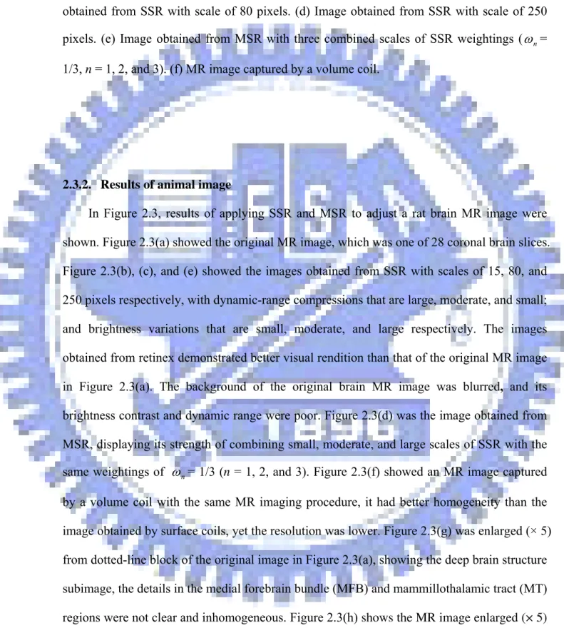
(37) . 2.3. Experimental results. 2.3.1. Results of phantom image. The performance of our retinex algorithm was assessed by determining the parameters for a test series of MR images of the phantom, with dimensions of 256 × 256 pixels and 16-bit quantization. The dynamic-range compression and brightness constancy were determined in the MR images of the test series, based on postprocessing by the retinex method. Figure 2.2 showed the results of using SSR and MSR to correct for the inhomogeneity of an MR image of the phantom. The original MR image was shown in Figure 2.2(a), which exhibited inhomogeneity, nonuniformity, low brightness, and a large dynamic range. SSR with a scale of every 10 pixels between 0 and 255 was used to analyze the series of phantom images. SSR with a scale of 15 pixels was also applied in this test. Figure 2.2(b), (c), and (d) illustrated the successful reductions in intensity inhomogeneity of the phantom images using SSR with scales of 15, 80, and 250 pixels respectively. The images in Figure 2.2(b), (c), and (d) showed dynamic-range compressions and brightness were large, moderate, and small, respectively, which indicated the dynamic-range compression increased when the SSR scale decreased. Figure 2.2(e) showed the image obtained from MSR by combining three scales of SSR weightings ( ω n = 1/3, n = 1, 2, and 3), where the three scales of SSR were 15, 80, and 250 pixels as used by Jobson et al. [82, 85]. The images obtained from the retinex algorithms were of higher quality than the original phantom image. Also, Figure 2.2(f) showed an MR image captured by a volume coil as a receiver with the same MR imaging procedures and parameters. Comparison of Figure 2.2(e) and (f) revealed that MSR successfully corrected the original MR phantom image.. - 25 -.

(38) . - 26 -.

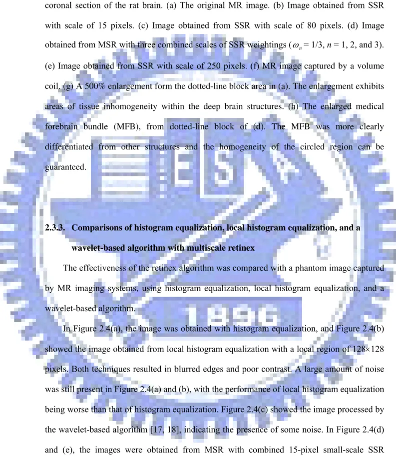
(39) . Figure 2.2 Corrected MR images of a phantom demonstrating the performance of retinex. (a). The original MR image. (b) Image obtained from SSR with scale of 15 pixels. (c) Image obtained from SSR with scale of 80 pixels. (d) Image obtained from SSR with scale of 250 pixels. (e) Image obtained from MSR with three combined scales of SSR weightings ( ω n = 1/3, n = 1, 2, and 3). (f) MR image captured by a volume coil.. 2.3.2. Results of animal image. In Figure 2.3, results of applying SSR and MSR to adjust a rat brain MR image were shown. Figure 2.3(a) showed the original MR image, which was one of 28 coronal brain slices. Figure 2.3(b), (c), and (e) showed the images obtained from SSR with scales of 15, 80, and 250 pixels respectively, with dynamic-range compressions that are large, moderate, and small; and brightness variations that are small, moderate, and large respectively. The images obtained from retinex demonstrated better visual rendition than that of the original MR image in Figure 2.3(a). The background of the original brain MR image was blurred, and its brightness contrast and dynamic range were poor. Figure 2.3(d) was the image obtained from MSR, displaying its strength of combining small, moderate, and large scales of SSR with the same weightings of ω n = 1/3 (n = 1, 2, and 3). Figure 2.3(f) showed an MR image captured by a volume coil with the same MR imaging procedure, it had better homogeneity than the image obtained by surface coils, yet the resolution was lower. Figure 2.3(g) was enlarged (× 5) from dotted-line block of the original image in Figure 2.3(a), showing the deep brain structure subimage, the details in the medial forebrain bundle (MFB) and mammillothalamic tract (MT) regions were not clear and inhomogeneous. Figure 2.3(h) shows the MR image enlarged (× 5) from dotted-line block of Figure 2.3(d) from MSR, regions (MFB and MT) circled with dotted-curve demonstrated better homogeneity and clarity. Figure 2.3(h) exhibits clearer deep - 27 -.

(40) . anatomical structures from MSR than Figure 2.3(g) from original image. The MSR clearly improved the quality, relative to that of the original MR image. Comparing among the original MR image, the image captured by a volume coil and the image obtained from the retinex algorithm revealed that the last method showed the best performance in terms of brightness, dynamic-range compression, and overall visual rendition.. - 28 -.

(41) . - 29 -.

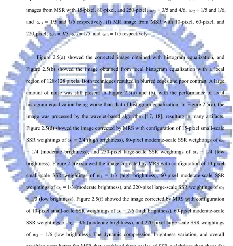
(42) . Figure 2.3 Performance of the retinex was demonstrated with adjusted MR images of a. coronal section of the rat brain. (a) The original MR image. (b) Image obtained from SSR with scale of 15 pixels. (c) Image obtained from SSR with scale of 80 pixels. (d) Image obtained from MSR with three combined scales of SSR weightings ( ω n = 1/3, n = 1, 2, and 3). (e) Image obtained from SSR with scale of 250 pixels. (f) MR image captured by a volume coil. (g) A 500% enlargement form the dotted-line block area in (a). The enlargement exhibits areas of tissue inhomogeneity within the deep brain structures. (h) The enlarged medical forebrain bundle (MFB), from dotted-line block of (d). The MFB was more clearly differentiated from other structures and the homogeneity of the circled region can be guaranteed. 2.3.3. Comparisons of histogram equalization, local histogram equalization, and a wavelet-based algorithm with multiscale retinex. The effectiveness of the retinex algorithm was compared with a phantom image captured by MR imaging systems, using histogram equalization, local histogram equalization, and a wavelet-based algorithm. In Figure 2.4(a), the image was obtained with histogram equalization, and Figure 2.4(b) showed the image obtained from local histogram equalization with a local region of 128×128 pixels. Both techniques resulted in blurred edges and poor contrast. A large amount of noise was still present in Figure 2.4(a) and (b), with the performance of local histogram equalization being worse than that of histogram equalization. Figure 2.4(c) showed the image processed by the wavelet-based algorithm [17, 18], indicating the presence of some noise. In Figure 2.4(d) and (e), the images were obtained from MSR with combined 15-pixel small-scale SSR weightings of ω1 = 3/5 and 4/6; 80-pixel moderate-scale SSR weightings of ω2 = 1/5 and 1/6; and 250-pixel large-scale SSR weightings of ω3 = 1/5 and 1/6 respectively. Figure 2.4(f) - 30 -.

(43) . showed the image obtained from MSR with combined 10-pixel small-scale SSR weightings of ω1 = 3/5; 60-pixel moderate-scale SSR weightings of ω2 = 1/5; and 220-pixel large-scale SSR weightings of ω3 = 1/5. All phantom figures in Figure 2.4 displayed clear deep structures and edges. The MSR algorithm exhibited better visual rendition than histogram equalization, local histogram equalization, and the wavelet-based algorithm. The performance of MSR was also compared with those of histogram equalization, local histogram equalization, and the wavelet-based algorithm on an MR image of rat brain.. - 31 -.

(44) . - 32 -.

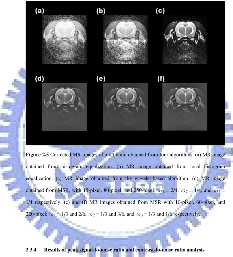
(45) . Figure 2.4 Corrected MR images of a phantom, obtained via four methods. (a) MR image. obtained from histogram equalization. (b) MR image obtained from local histogram equalization. (c) MR image obtained with the wavelet-based algorithm. (d) and (e) MR images from MSR with 15-pixel, 80-pixel, and 250-pixel; ω1 = 3/5 and 4/6, ω2 = 1/5 and 1/6, and ω3 = 1/5 and 1/6 respectively. (f) MR image from MSR with 10-pixel, 60-pixel, and 220-pixel; ω1 = 3/5, ω2 = 1/5, and ω3 = 1/5 respectively.. Figure 2.5(a) showed the corrected image obtained with histogram equalization, and Figure 2.5(b) showed the image obtained from local histogram equalization with a local region of 128×128 pixels. Both techniques resulted in blurred edges and poor contrast. A large amount of noise was still present in Figure 2.5(a) and (b), with the performance of local histogram equalization being worse than that of histogram equalization. In Figure 2.5(c), the image was processed by the wavelet-based algorithm [17, 18], resulting in many artifacts. Figure 2.5(d) showed the image corrected by MRS with configuration of 15-pixel small-scale SSR weightings of ω1 = 2/4 (high brightness), 80-pixel moderate-scale SSR weightings of ω2 = 1/4 (moderate brightness), and 250-pixel large-scale SSR weightings of ω3 = 1/4 (low brightness). Figure 2.5(e) showed the image corrected by MRS with configuration of 10-pixel small-scale SSR weightings of ω1 = 1/3 (high brightness), 60-pixel moderate-scale SSR weightings of ω2 = 1/3 (moderate brightness), and 220-pixel large-scale SSR weightings of ω3 = 1/3 (low brightness). Figure 2.5(f) showed the image corrected by MRS with configuration of 10-pixel small-scale SSR weightings of ω1 = 2/6 (high brightness), 60-pixel moderate-scale SSR weightings of ω2 = 3/6 (moderate brightness), and 220-pixel large-scale SSR weightings of ω3 = 1/6 (low brightness). The dynamic compression, brightness variation, and overall rendition were better for MSR that combined three scales of SSR weightings than those for histogram equalization, local histogram equalization, or the wavelet-based algorithm alone. All rat brain figures in Figure 3.5 displayed clear deep anatomy structures and edges. - 33 -.